A Binary Ensemble Classifier for High-Frequency Trading Everton Silva Programa de P6s-Graduas;ao em Ciencia da Computas;ao Universidade Federal de Minas Gerais (UFMG) Belo Horizonte, Brazil
[email protected]
Humberto Brandao Financial Computing Centre (FCC), ICEx, Universidade Federal de Alfenas (UNIFAL-MG) Alfenas, Brazil
[email protected] Adriano C. M. Pereira Departamento de Ciencia da Computas;ao Universidade Federal de Minas Gerais (UFMG) Belo Horizonte, Brazil
[email protected]
Douglas Castilho Laborat6rio de Tecnologia da Informas;ao Instituto Federal do SuI de Minas Gerais - Campus Passos Passos, Brazil
[email protected] Ahstract-The aim of this study was to model and use machine learning techniques to maximize the chance of a market maker be executed successfully in a stock market, that is, when their bid and ask orders are filled at the desired prices. In this context, a binary ensemble classifier was created to decide whether, at a specific time, is or not propitious to start a new market making process. Conducting the study over a large volume of data for high-frequency traders, we showed that the new proposed ensemble classifier was able to improve the efficiency of the isolated models and the precision of the models are better than random decision makers.
I.
INTRODUCTION
On-line trading has been transforming the investment world at a dizzying speed. Before the advent of computers, the stock market investors perform their operations based mainly on intuition. With the growth of investments and stock trading, a continued search for better tools to accurately predict the stock market has become necessary in order to increase profits and reduce risks. Currently, there are several algorithmic traders that use electronic platforms for inserting orders in financial markets without the human intervention [1]. A particular type of algorithmic trading is high-frequency trading (HFT). This category of trading emerged in the last decade and recently has gained attention from academic researches. Studies suggested that HFT accounted for 50-75% of all US equity trading volume in the recent years [2]. The most common type of HFT is by performing a process called market making [3], [4], [5]. A market making process places a buy and a sell limit orders, simultaneously or not, with the purpose of making profit through small fluctuations in stock prices. As well as other decision-making processes, machine learn ing techniques can support the high-frequency traders. An important decision-making process in HFT is to know when the algo trader needs to trigger a new market maker. If the market maker is configured to perform a profitable operation expecting a small increase in the stock price, but the price goes to the opposite side, then losses can be accumulated. This is a very challenging problem because it involves to predict small trends in the stock prices for short periods of time.
help algo traders in the high-frequency field, getting good predictions for short time windows, when the trading system tries to identify a small trend in the stock prices. Although it has been successful in predicting small uptrends, this past research has not been capable to get profits in a realistic simulator, surpassing the real market fees. Obviously, this is a sine qua non condition to apply an intelligent model in a stock exchange. During the last year, we realized that a good binary classifier for the problem studied in this research must have a high precision in the class 1 and there is no problem if the system has a low precision in the class 0, considering that class 1 is when the trading system needs to trigger a new market maker, to make a profit, and class 0 is otherwise. The reason of this conclusion is because when the system makes mistakes in the class 0, it does not lose money. This situation is better than if compared when the system makes mistakes in the class 1, that can cause financial loses. If the system has a high precision in the class 1 (i.e., operate) and a low precision in the class 0, there is a higher chance to make money, different to the otherwise. After this conclusion, our efforts were to create a binary classifier with a high precision in the class 1, without regard to the accuracy achieved in the class 0, but with a reasonable amount of triggers to ensure a high turnover of capital, that is very important to classify the trade system as a high-frequency trader. If the trade system is classified as a high-frequency trader, the majority of stock exchanges gives some discounts in fees, that is important when the system can achieve only small gains for each pair of orders, in function of the short time windows to close positions. In this context, the new classifier presented in this work has contributions in two main aspects: (i) considering that the uptrends prediction is hard to do, the precision of the ensemble in the class 1 was greater than the class 1 distribution for all analyzed assets; (ii) the results of the ensemble were better than the isolated artificial intelligence models. II.
A. Summary of the main contribution of this work To understand the history of the research, in our previous model [6], we showed that an artificial neural network could
978-1-4799-1959-8/15/$31.00 @2015
IEEE
ALGO TR ADING AND COMPUTATION AL INTELLIGENCE
The automation of strategies is not a new process. Algo traders have existed since that markets have become electronic in the mid-80s [4]. The Internet also played an importan�
role in the popularization of algo traders. The evolution of technology to support algo traders happened in parallel with the progress of computational intelligence techniques during the last 30 years. As in other areas, a natural step of scientific community was to investigate a large number of techniques to help systems to make automatic decisions in the stock exchanges. By the end of the 90s, a large number of researches were developed trying to predict the time series of prices, liquidity and volatility. The most of them discretizing the time in daily, weekly, biweekly or monthly intervals. With the technological progress in the last decade, a new field of trading was coined and well defined: High-Frequency Trading; In this category, algo traders can buy or sell shares in less than one millisecond. It is interesting for two main reasons: 1) The algorithms can turnover capital with a short amount of money in their accounts; 2) Closing positions in short time intervals, strategies can control the risk easily and satisfactorily. It is because the value of the portfolio is less dependent on the stock price oscillations. A. Related work All algorithms of high-frequency trading act as day traders. It means that they buy and sell shares at the same day. But, day traders have been around since the inception of the stock market in 1792 [7]. Human beings have speculated on prices since the dawn of currency, and this trend will continue regardless of the state of the market. Moreover, before the advent of computers, the stock market investors made their negotiations based mainly on intuition. With the growth of investments and stock trading, a continued search for better tools to accurately predict the stock market has become necessary in order to increase profits and reduce losses. Recently, several market prediction models and computa tional intelligence techniques have been developed in order to support investment decisions for intraday operations in stock markets, such as market maker and HFT, and for middle or long-term strategies. For HFT, the Artificial Intelligence field has been investigated using Artificial Neural Networks (ANNs) [8] and Fuzzy Systems [9], [10]. Statistical regression, technical analysis, fundamental anal ysis, time series analysis, chaos theory are some of the techniques that have been adopted to predict the market trends [11]. However, these techniques are not able to generate consistently a correct prediction of the stock market, generating many doubts among analysts about the use of many of these approaches [12]. Thus, predicting the change of price move ment in stock markets and trying to make correct investment decisions is one of the main challenges in this context [13]. The first significant study on the application of neural network models for prediction of the financial market was published by White [14]. He presented some results, using techniques of modeling and neural network learning to dis cover and decode nonlinear regularities in stock price move ments. The study was focused on the stocks of IBM and with granularity of Daily returns. Having to deal with the main features of economic data, the statistical inference played an important role and technical changes were necessary to the learning process. After this study, several research efforts have
been conducted to examine the effectiveness of prediction of neural network models in stock markets [15], [16] The work [12] reports that the application of neural net works to predict the financial market variables and the use of technical analysis and fundamental analysis is a predomi nant factor for stock market predicting. The article presents a hybridized approach that combines the use of variables of technical and fundamental analysis as indicators of the stock market to predict future stock prices. The obtained results showed significant improvement compared to using only variables of technical analysis. In another context, the prediction approach was also satisfactory as a guide for traders and investors in making qualitative decisions. In [17], they used algorithms for training models to predict Standard&Poors 500 Index and then compared the results using a genetic programming (GP) approach. [18] present a survey of the literature on prediction mechanisms, including prediction markets and peer prediction systems. They focus on the design process, highlighting the objectives and properties that are important in the design of good prediction mechanisms. In the HFT context, the approach in [8] used ANN model with popular technical indicators to predict trading signals, which can be useful to perform day trading. The set used to build the model is the high frequency ticks of intra-day stocks from some industry sectors in the Indonesia Stock Exchange Market. The study compares the performance of the model with a naive buy-and-hold strategy and the maximum profit profile. The experimental results showed that the proposed model performed better than the naive strategy. Thus, the author concluded that the ANN is useful to generate trading signal predictors for intra-day traders from the high frequency dataset. [19] investigate the implications of HFT on market ef ficiency and price discovery by using state-space models and real-life one-minute high-frequency data of the six most traded currency pairs worldwide. The authors identified significant evidence that HFT enhances market efficiency and has a beneficial role in price discovery by trading in the direction of the permanent component of the state-space model and in the opposite direction of its transitory component. III.
MET HODOLOG Y
This section describes the methodology applied in this work, which is illustrated by Figure 1. Each step will be explained in the next subsections. A. Data Gathering The data set used in this work consists of real data from the Brazilian Stock Exchange (BM&F Bovespa), which is the 8th largest one in the world. This data set was gathered from one of the financial data vendor, which provides data to financial firms, traders and investors. It contains information about each symbol from this stock market. As showed in Figure 1, this gathered data defines our experimental data set (Market Data). B. Data Preprocessing The market data gathered in the last step is preprocessed in order to produce the candlesticks. A candlestick represents the price variation of a symbol or action during a time unit
A �U
Data Preprocessing -----I��
Data Gathering �
U
Stock1
r==-1 LJ
Stock 2
U
Market Data
Stock Exchange
Stockn
Candlestick Data
Ifdf,lf,lf,lfslt.lf71·..EJ Ifdt,lf,!f,lfslidt,l ...EJ Ifdf,lf,!f,lfslt.!f71·"EJ Data Set / Features
..
Fig. 1.
Market Simulation
I tIP. I
..
Financial Results
Results and Performance
and Analysis
Evaluation Measures
&""000"' execution
Experimental Setup
Proposed Methodology - Steps
(e.g., 15 minutes), where: Open is the first trade price in the period; Close is the last trade price in the period; High is the higher trade price in the period and; Low is the lower trade price in the period. We use a different way to generate the candlesticks. The candlesticks do not synthesize a range of a mutually exclusive time. They use the concept of rolling window, defined in [6]. Consider that a granularity of a candlestick is, for example, 5 time units. In common representations, each candlestick summarizes this period in a static and unique way, i.e, it starts at time to and comprises information until the time t4' Another candlestick would start at t5 and end at tg, and so forth. Thus, they do not have information in common with each other, being mutually exclusive. As showed in Figure 2, using the rolling window concept applied to the same granularity of 5 units, there would be a first candlestick starting at time to and ending at time t4, but the second one would have start in time tl and finalization in time t5, and a third one would have start in time t2 and finalization in time t6. Data preprocessing execution generates the candlesticks for each symbol (see Figure I - Candlestick Data). The candlesticks are processed and treated to extract data features, as will be described in next section. C. Data Processing and Treatment In order to decide the best instant to initialize a market maker, we used machine learning techniques to perform the uptrend prediction in the price of a given asset. For example, if we want to make a profit of R$ x (x cents of Rea!), a limit order to buy and sell a stock are placed simultaneously to the market with the following prices: R$ x (cents of Real) and R$ x + y (cents of Real), respectively. It is how a market maker strategy works. In this context, we expected that the asset price goes up and both orders are executed. The challenge is to know when this operation should be initialized. For this purpose, we use machine learning techniques to try to predict this uptrend for a
given time interval. Note that the value of the rolling window used to generate the indicators is the same time interval for the uptrend prediction. (Figure 2). To perform this prediction, we modeled and built a set of features that are used as inputs to the machine learning techniques. These features are composed by technical analysis indicators, followed by a binary attribute (0 or 1), which previews if price is going to have the desired variation. The value 1 indicates that the market maker must be initialized and 0, the opposite case. The indicators used as features are obtained through processing of candlesticks and are presented in Section III-CI. Figure 2 illustrates the methodology for the generation of features used by the machine learning techniques. In the period defined as Generating Indicators, we generate the technical analysis indicators, which make up the features. In order to verify that the stock price is going to have the expected positive variation (uptrend), we only check the candlestick that contains the information of future quote. For example, considering that the rolling window value is 5 units of time. If we want to verify whether a market maker can be started in time t5, we check whether the desired positive variation occurs in the candlestick tg, because it contains information of the price variation for the time interval between t5 and tg. Such verification is performed as defined by Equation 1:
var
=
High(tj) - OpenPrice(ti),
(1)
where ti is the instant of time where the operation is started and tj is the instant of time equivalent to the size of ti + rollingWindow. OpenPrice(ti) is the opening price of the candlestick at time ti and High(tj) is the highest price of the candlestick reached in the range of ti until tj. Finally, var' contains the variation between the maximum price and the opening price in this range.
D. Machine Learning Techniques and Experimental Setup The experiments were performed following a similar con cept to the rolling window used in the processing of candle sticks. We separate the generated data set in the previous step (III-C) into training and testing sets as follows: we use a period containing n days to train the models and we tested their ability to forecast on n+ 1. One day i comprises the features generated using candlesticks this day exclusively.
Fig. 2.
Building the prediction model
1) Technical Analysis Indicators - Features: The proposed methodology considers the characterization and analysis of some technical analysis indicators. An indicator can be defined as a series of data points, which are derived from the price information of stocks applied to a mathematical formula. The data set of price attributes of each stock is a combination of the price of opening, closing, maximum and minimum over a period of time [20]. Thus, the set of features used as input for the machine learning techniques will be the different indicators calculated for a time period (candlestick). Market analysts generally use one or more indicators for their analysis [20]. These indicators are usually chosen by eval uating the accuracy of the model. Most often, many indicators are omitted and a good model can never be discovered for a particular stock, i.e., the more information you have, the better will be the outcome of the model. If the input data are not relevant to the desired output, probably the model will not learn well the associations between the data input and output. Thus, the first step is to use a set of indicators commonly used in traditional technical analysis. In order to specify the attributes or indicators to adopt in the experiment, we previ ously performed a general characterization of them, observing the typical behavior of each attribute and the historical stock oscillation, trying to infer which of them has potential to be used in our model. ; Next, we list each indicator used as input in our model: I Relative Strength Index (RSI), Moving Average, Exponential Moving Average, Moving Average Con vergenceJDivergence (MACD), Average Directional Movement Index (ADX), Aroon Indicator, Bollinger Bands, Commodity Channel Index (CCI), Chande Momentum Oscillator (CMO), Rate of Change (ROC). Note that an indicator can generate more than one feature. For example, the Aroon indicator is made up of two lines: one line is called aroon up, which measures the strength of the uptrend, and the other line is called aroon down, which measures the downtrend. Thus, each pattern consists of 26 features followed by a binary attribute (l or 0). After data processing and treatment, we have the new data set (see Figure 1 - Data Set / Features). This data set is used as input to the computational intelligence techniques.
I for more information about these technical indicators, http://www. stockcharts.com, http://www.investopedia.com and [20]
see
Figure 3 illustrates the generation of training and testing sets using a rolling window of 4 days. Following this example, a training set is implemented (days Do , D1, D2 and D3) to build up a model, while a test set (D4) is to validate the model built. The window size N is fixed and the window moves to the right one day each time while discarding one day on the left side. For each window offset, a new model is generated for the next day's prediction. In our experiments we used different rolling window sizes for trials of the back testing. Therefore, different models were generated with these setups and we evaluated the effectiveness of each one using some performance measures. The next section presents a brief description of machine learning techniques used in this research.
I
Training Set
Test Set
It----t
GGGG G GGGGG
Fig. 3.
Training and test set
1) Machine Learning Techniques: In order to verify if the stock price presents a desired variation in a time interval, we use two machine learning techniques. •
Multilayer Perceptron - MLP: consists of several lay ers of simple elements (or two states) of sigmoidal processing, or neurons that interact by using weighted connections [21]. After an input layer, there are typ ically any number of intermediate layers, or hidden, followed by an output layer [22], [23]. MLP uses a supervised learning technique called backpropagation for training the network. It is a modification of the standard linear perceptron and can distinguish data that are not linearly separable.
•
Ensemble: an ensemble of classifiers is a set of classi fiers whose individual decisions are combined in some way (typically by weighted or unweighted voting) to classify new examples. Ensemble methods uses this combination to obtain better predictive performance than could be obtained from any of the individual classifiers that make them up [24]. Many methods for constructing ensembles have been developed, which can be applied to many different learning algorithms. More information can be found in [24], [25] and [26]. In this work we built an ensemble combining two MLP decisions. For example, if the output of both
models belongs to class 1, then the output ensemble is also 1. The same method is applied to class O. E. Experimental Execution This step is to perform the execution for all experimental setups generated in the previous stage. The result of each experimental setup was evaluated using different performance measures. 1) Performance Measures for Classification: Different per formance measures are available to evaluate the effectiveness of a classifier. In a classification problem, a classifier labels examples as positive or negative. The decision taken by the classifier can be represented in a structure known as confusion matrix or contingency table [27]. The confusion matrix is often used to organize and display information used to evaluate the performance of an algorithm, usually a supervised learning algorithm. Each column of the matrix represents the instances of a predicted class, while each row represents the case in a real class [28]. The performance measures are derived from information contained in the confusion matrix. In this work, we used different performance measures to evaluate the classifiers, that is, its ability to take the right classification decisions. More information about performance measures can be found in [29]. The main performance measures used in this work were: true positive (T P), false negative (F N), false positive (F P), true negative (TN) and precision. T P is when a trigger (market maker execution) was correctly classified (the buy and sell orders are filled), while F P is when a trigger was incorrectly classified. The F N is when there exists a trigger, but the classifier does not identify it. In this case, we lose an opportunity. TN is when there is not a trigger and the classifier indicates that correctly. However, we are not evaluating this metric because we are interested only in scenarios that provide some profit. In this context, among the performance measures listed, we gave more importance to precision, because they establish the relationship between T P and F P. Precision is the number of correctly classified positive examples (T P) divided by the number of examples labeled by the classifier as positive (T P + F P). The experiment results are presented in the section IV. For each test day, it is obtained the precision for each classifier. In order to analyze and discuss the results, tables and CDF (cumulative distribution function) charts are synthesized from the obtained precision. The main objective of these analysis and discussion is to identify the best classifier, just as the best setup: training rolling window and prediction time window. Then, we use a realistic HFT simulator to evaluate the financial result of the predictions (triggers) obtained by the machine learning techniques used in this work. F.
Market Simulation
To study, understand and evaluate the quality of the use of classifiers at BM&FBOVESPA, and analyze the hypotheses proposed in this work, the stock market, the broker, the communication structure, and other key components were emulated using a technique called Discrete-Event Simulation. This simulator allows us to perform tests without the need to buy and sell shares in the real market.
Our market simulator is based on intraday data, able to receive and execute orders, and also compute the priority of an order in the order book that has not been executed or canceled. The system accepts limit orders, market orders and cancellations. The best classifiers were used in the simulator, and as a result we will present an analysis of the financial return during our test period (see Section IV). IV.
RESULTS AND DISCUSSION
The data used for the experiments consists of a real data set from the Brazilian Stock Exchange (BM&FBOVESPA). It contains all information of 51 days from January to April 2015, including orders, trades, changes in the order book and all other delivered data by the FIX Protocol2. It is important to be clear that this number of days is considered satisfactory for experimental analysis because the data volume is large considering that the problem is about HFT, because we can generate thousands of patterns with few days in the data set [4]. The symbols of the companies analysed in this article include: ITAU UNIBANCO HOLDING S.A. (ITUB4), Petroleo Brasileiro s.A. - Petrobras (PETR4) and VALE s.A. (VALES). These companies are part of a select group of Brazilian symbols (BM&FBOVESPA), called Bovespa Index (iBov or IBovespa)3. The Bovespa Index is composed by a theoretical portfolio with the stocks that accounted for 80% of the volume traded in the last 12 months and that were traded at least on 80% of the trading days. It is revised quarterly, in order to keep its representativeness of the volume traded and on average the components of Ibovespa represent 70% of all the stocks value traded. The companies that participate in Bovespa Index have greater marketability and representativeness of the Brazilian Stock Exchange. Thus, the stocks that we choose for our experiments are considered liquid and very important in the Brazilian Stock Exchange. In high-frequency trading, it is common to perform various trades a day, trying to get a small gain on average. In this context, our experiment aims to predict whether a particular stock will get a positive variation (uptrend) greater or equal to a predefined value: R$ 0.02 (two cents of Real). The Real (R$ symbol) is the current Brazilian currency. We are interested in this variation because we can earn R$ 0.02 for each share negotiated, placing a bid and an ask order at the price R$x and R$x + 0.02, respectively. Thus, the buying and selling of round lot shares (100), gives us a gain of R$ 2.00 for each uptrend detected with success. Repeating this process hundreds or thousands of times during a trading session, the algo trader can get considerable gains. This is a simple logic about high frequency trading. This value of R$ 0.02 was obtained through analysis of operation costs in the Brazilian Stock Exchange. This value also depends of the share value. This value can be higher or lower than R$ 0.02, depending on the stock price. In this work we used only R$ 0.02 because all analysed symbols were adapted for this value. We conduct several trials of back-testing with different training rolling window sizes and predict time window sizes. 2FIX Protocol: www.fixtradingcommunity.org 3 Ibovespa index: http://www.bmfbovespa.com.brlindices/Resumolndice.aspx? Indice=lbovespa&ldioma=en-us
TABLE l. TW Size
Technique
TW5
MLP_1
PERFORMANCE MEASURE FOR ITUB4 FP
0.45
51.20
56.43
0.50
0.61
52.97
58.00
0.50
0.62
29.54
30.83
0.51
0.62
110.89
83.03
0.58
0.67
112.26
90.34
0.58
0.68
77.60
58.94
0.60
0.70 0.70
MLP
MLP
0.55
MLP_1 ENSEMBLE
TWlO
MLP
0.59
MLP_1 ENSEMBLE TABLE II.
TW Size
Technique
TW5
MLP_1
MLP
MLP MLP_1
Distribution
0.21
0.29
ENSEMBLE TWlO
MLP MLP_1
157.94
109.03
0.60
154.83
104.14
0.61
0.71
130.49
88.63
0.61
0.71
PERFORMANCE MEASURE FOR PETR4
ENSEMBLE TW8
Simulation Precision
TP
ENSEMBLE TW8
Model Precision
Distribution
0.33
ENSEMBLE
For training rolling window size, we used 1 day, 5, 8, 10, 14, and 20 days. The predict time window gets the following values: 5, 8 and 10 minutes. In this context, we find that using 14 days of training, the generated models have a better performance in the next test day. Next we present the best results obtained through tables and CDF (Cumulative Distri bution Function) charts, which allows to easy compare the distribution of frequency of the precision measures of each model's result. Tables I and II present the results for two symbols, ITUB4 e PETR4, respectively. These are the average results of all test days. The first column is the predict time window value (TW). For each TW, we have the performance results for each technique: two MLPs (MLP and MLP_1) and the Ensemble. We can conclude from the results that: the precision of the machine learning models are always significantly greater than the aleatory model (which follows the distribution of class 1); the best results (highlighted in bold face) were achieved by the Ensemble, which sometimes are similar to MLP_1. Fur thermore, we can observe that simulation precision is greater than model precision, which is nice because guaratee better results in the realistic HFT simulation. This can be explained by the fact that some FP triggers that would led to losses in the classification model are not executed in simulation, improving the precision in simulation and, consequently, the financial results of it. Figures 4, 5 and 6 are presented the Cumulative Distribu tion Function analysis to compare the behavior of the class 1 distribution (market maker triggers), the ensemble model and the realistic simulation using the ensemble model as trigger to
TP
FP
Model Precision
Simulation Precision
16.68
3l.24
0.34
0.38
15.14
3l.00
0.33
0.43
8.53
13.75
0.40
0.44
28.03
46.59
0.38
0.44
29.46
49.78
0.38
0.43
17.60
27.86
0.40
0.45
35.74
56.80
0.37
0.42
4l.89
66.23
0.35
0.42
25.00
35.66
0.37
0.42
start a new market maker execution. The class 1 distribution can also be understood as a random model. This analysis are summarized for different time window sizes and each evaluated asset. The results comprises the entire period used for the test set. We can see that the ensemble model behavior is better than the aleatory distribution. We can also see that the results in simulation are better than the ensemble model, because some executions work correctly in real simulation, even the model saying that the share price would not uptrend. The higher the TW value, the results between the ensemble and the distribution model come closest. However, it increases the risk of the operation, as shown in Figure 7 (increases the accuracy rate, but also increases the amount of losses). As example in ITUB4 (TW 8), the ensemble model distri bution has 80% with accuracy rate above 50%, while the real istic simulation is approximately 98%. Also in ITUB4, when compared to TW 10, the ensemble model has approximately 91 % of the distribution above 50% accuracy. In order to evaluate the real financial results achieved by our algotrading strategies, we perform a realistic simulation using real order book time series data. As expected by the previous analyzed results, the best results were obtained by the proposed Ensemble model, which combines two distinct neural networks. Figure 7 shows the financial analysis of the symbols ITUB4, PETR4, and VALE5, respectively, for the different time window sizes (i.e., 5, 8 and 10). Note that we applied a zoom-in the curves, where axis x represents the financial value for a trigger (in R$), thus all gains up to 1 in axis yare concentrated in point 2 of x, which corresponds to financial gains obtained by successful triggers (true positives).
0.8
r
0.8
r
6
J: 0.4
6
J: 0.4
0.2
0.2 0.&
0.9
(a) ITUB4 - TW5 Fig. 4.
(c) ITUB4- TWIO
(b) ITUB4 - TW8
Cumulative Distribution Function for different time window sizes - ITUB4; Distribution (aleatory), Model (ensemble), Simulation (ensemble simulated).
0.8
0.8
0.8
� O.6 �
! 0.4 0.2
0.2
-Aleatory Distribution -Ensemble Model -Ensemble Simulated
-Aleatory Distribution -Ensemble Model
���--� 0.2�� 0.�3� 0�.4�� 0.5�� 0�.6�0�.7�0� .� &�0�.9�
-Alcalory Disiriblllion -Ensemble Model
0.8 0.9
0.& 0.9
(a) PETR4 - TW5 Fig. 5.
0.2
(c) PRTR4- TWIO
(b) PETR4 - TW8
Cumulative Distribution Function for different time window sizes - PETR4; Distribution (aleatory), Model (ensemble), Simulation (ensemble simulated).
0.8
r
0.8
r
6
J: 0.4
0.8
� O.6 ! J: 0.4
6
J: 0.4
0.2
0.2 -Ensemble Simulated
0.8
(a) VALE5 - TW5 Fig. 6.
(b) VALE5 - TW8
0.9
(c) VALE5- TWIO
Cumulative Distribution Function for different time window sizes - VALE5; Distribution (aleatory), Model (ensemble), Simulation (ensemble simulated).
0.35 0.3 30.25 � 0.2 �
lO.\5 0.1 0.05
(a) ITUB4 Fig. 7.
(b) PETR4
(c) VALE5
Financial Results for different time window sizes
As can be observed from these analyses, for all symbols, the best positive results (profit triggers) are achieved by higher
time windows (granularities 10 and 8), except for PETR4. However, in these cases, the amount of financial losses are
also higher, since the operation risk is higher because of the occurrence of false positives (F P). For ITUB4 (Figure 7(a)) we obtained from 64% (time window 5) to 71% (time window 10) of positive triggers. For PETR4 (Figure 7(b)) we obtained from 48% (time window 5) to 51% (time window 10) of positive triggers. For ITUB4 (Figure 7(c)) we obtained from 45% (time window 5) to 60% (time window 10) of positive triggers. These results are promise, since our machine learning model has already achieved a good amount of positive triggers, but as future work we need to minimize the FP triggers in order to avoid higher losses, which we hope will provide feasible and profitable results for high frequency trading. V.
FIN AL REM ARKS AND CONCLUSIONS
As the main contribution, a binary ensemble classifier was created to decide whether, at a specific time, it is propitious or not to start a new market making process in high-frequency algo traders. We showed that the new proposed ensemble classifier, that mixes two artificial neural networks, was able to do an uptrend prediction. Its precision was greater than the class 1 distribution for all analyzed assets. Furthermore, the results of the ensemble were better than the isolated neural networks. The tests were conducted using a large data set for high frequency trading, that includes, all order book information, single orders, trades, modifying and canceling orders. It con textualizes a new contribution in the High-Frequency Trading field, where the market making algorithms have a special importance. The proposed methodology is generic and it can be applied for different financial time series data sets, with the flexibility to choose different indicators to build the set of features for the model, besides evaluating different computational intelligent techniques. The achieved results and findings have opened new re search directions, thus we foresee the following opportunities for future work: •
•
Evaluate if downtrend can also be identified with a similar methodology in order to complement this work. This could increase the liquidity of the market; The use of neural networks as a trigger for other types of strategies in High-Frequency Trading (e.g., Statistical Arbitrage). ACKNOWLEDGMENT
[3]
[4] [5] [6]
[7] [8] [9] [10]
[II]
[12] [13] [14] [15]
[16]
[17] [18] [19]
[20] [21] [22] [23] [24] [25]
[27]
REFERENCES
[28]
T. C. Lin, "The new investor," UCLA L. Rev., vol. 60, pp. 678-778, 2013.
[2]
F. Zhang, "High-Frequency trading, stock volatility, and price discovery," Social Science Research Network Working Paper Series, Oct. 2010. [Online]. Available: http://ssrn.comJabstract=1691679
A. Kablan and W. Ng, "High frequency trading using fuzzy momentum analysis," in Proceedings of the World Congress on Engineering, vol. I, 2010. A. Kablan, "Adaptive neuro fuzzy inference systems for high frequency financial trading and forecasting," in Advanced Engineering Computing
and Applications in Sciences, 2009. ADVCOMP '09. Third International Conference on. IEEE, 2009, pp. 105-110.
This research was supported by the Brazilian National Institute of Science and Technology for the Web (CNPq grant numbers 57387112008-6 and 477709/2012-5), CAPES, CNPq, Finep, Fapemig and Oragon Tech.
[I]
B. Hagstromer and L. Norden, "The diversity of high-frequency traders," Journal of Financial Markets, vol. 16, no. 4, pp. 741 - 770, 2013, high-Frequency Trading. [Online]. Available: http://www.sciencedirect.com/science/article/pil/S1386418113000256 1. Aldridge, High-frequency trading: a practical guide to algorithmic strategies and trading systems. John Wiley & Sons, 2013. A. J. Menkveld, "High frequency trading and the new market makers," Journal of Financial Markets, vol. 16, no. 4, pp. 712 - 740, 2013, high-Frequency Trading. E. Silva, D. Castilho, A. Pereira, and H. Brandao, "A neural network based approach to support the market making strategies in high frequency trading," in Neural Networks (]JCNN), 2014 International Joint Conference on. IEEE, 2014, pp. 845-852. J. Lukeman, The Market Maker 's Edge. McGraw-Hill New York, 2000. E. F. Putra and R. Kosala, "Application of artificial neural networks to predict intraday trading signals," Recent Researches in E-Activities, pp. 174-179, 2011.
[26]
[29]
K. Ravichandran, P. Thirunavukarasu, R. Nallaswamy, and R. Babu, "Estimation of return on investment in share market through ann," Journal of Theoretical and Applied Iriformation Technology, vol. 3, 2005. A. Adebiyi Ayodele, O. Adebiyi Marion, and O. Otokiti Sunday, "Stock pnce prediction using neural network with hybridized market indicators." R. Thalheimer and M. M. Ali, "Time series analysis and portfolio selection: An application to mutual savings banks," Southern Economic Journal, pp. 821-837, 1979. H. White, "Economic prediction using neural networks: The case of ibm daily stock returns," in Neural Networks, 1988., IEEE International Conference on. IEEE, 1988, pp. 451-458. F. A. de Oliveira, C. N. Nobre, and L. E. Zarate, "Applying artificial neural networks to prediction of stock price and improvement of the directional prediction index - case study of petr4, petrobras, brazil," Expert Systems with Applications, vol. 40, no. 18, pp. 7596 - 7606, 2013. c. Evans, K. Pappas, and F. Xhafa, "Utilizing artificial neural networks and genetic algorithms to build an algo-trading model for intra-day foreign exchange speculation," Mathematical and Computer Modelling, vol. 58, no. 5, pp. 1249 - 1266, 2013. P. C. McCluskey, "Feedforward and recurrent neural networks and genetic programs for stock market and time series forecasting," Master 's thesis, Brown University, 1993. y. Chen and D. M. Pennock, "Designing markets for prediction." AI Magazine, vol. 31, no. 4, pp. 42-52, 2010. [Online]. Available: http://dblp.uni-trier.de/db/journals/aim/aim31. html#ChenPI0 Y. Manahov and R. Hudson, "The implications of high-frequency trading on market efficiency and price discovery," Applied Economics Letters, 2014. [Online]. Available: http://dx.doi. org/IO. 1080/13504851. 2014.914135 S. Thawornwong, C. H. Dagli, and D. L. Enke, "Using neural networks and technical analysis indicators for predicting stock trends," Intelligent Engineering Systems through Artificial Neural Networks, 2001. S. E. Fahlman and G. E. Hinton, "Connectionist architectures for artificial inteUigence," Computer;(United States), vol. 20, no. I, 1987. S. K. Pal and S. Mitra, "Multilayer perceptron, fuzzy sets, and clas sification," Neural Networks, IEEE Transactions on, vol. 3, no. 5, pp. 683-697, 1992. F. Rosenblatt, "Principles of neurodynamics. perceptrons and the theory of brain mechanisms," DTIC Document, Tech. Rep. , 1961. T. G. Dietterich, "Ensemble methods in machine learning," in Multiple classifier systems. Springer, 2000, pp. 1-15. J. Kittler, M. Hatef, R. P. Duin, and J. Matas, "On combining classi fiers," Pattern Analysis and Machine Intelligence, IEEE Transactions on, vol. 20, no. 3, pp. 226-239, 1998. L. l. Kuncheva, Combining pattern classifiers: methods and algorithms. John Wiley & Sons, 2004. J. Davis and M. Goadrich, "The relationship between precision-recall and roc curves," in Proceedings of the 23rd international conference on Machine learning. ACM, 2006, pp. 233-240. S. Y. Stehman, "Selecting and interpreting measures of thematic clas sification accuracy," Remote sensing of Environment, vol. 62, no. I, pp. 77-89, 1997. M. Sokolova and G. Lapalme, "A systematic analysis of performance measures for classification tasks," Information Processing & Manage ment, vol. 45, no. 4, pp. 427-437, 2009.