Optimization via simulation (OvS) is an exciting and fast developing area for both ... of a simulation model easily and try to observe the system performance ...
Proceedings of the 2009 Winter Simulation Conference M. D. Rossetti, R. R. Hill, B. Johansson, A. Dunkin, and R. G. Ingalls, eds.
A BRIEF INTRODUCTION TO OPTIMIZATION VIA SIMULATION L. Jeff Hong Department of Industrial Engineering and Logistics Management The Hong Kong University of Science and Technology Clear Water Bay, Hong Kong, China Barry L. Nelson
ABSTRACT
Department of Industrial Engineering and Management Sciences Northwestern University 2145 Sheridan, Evanston, IL, 60208, U.S.A.
Optimization via simulation (OvS) is an exciting and fast developing area for both research and practice. In this article, we introduce three types of OvS problems: the R&S problems, the continuous OvS problems and the discrete OvS problems, and discuss the issues and current research development for these problems. We also give some suggestions on how to use commercial OvS software in practice. 1
INTRODUCTION
Computer simulation is one of the most widely used operations research tools in practice. Every day, simulation users build simulation models to design and analyze complex systems. One feature of simulation is that one can change the parameters of a simulation model easily and try to observe the system performance under different sets of parameters. Therefore, it is natural to try to find the set of parameters that optimizes the system performance. This is what we call optimization via simulation (OvS). Because OvS requires simulating the system for multiple replications at multiple (possibly a very large number of) parameter settings, abundant computing power is necessary. Due to the rapid growth of computing power, OvS has become popular in recent years. Many practical problems can be formulated as an OvS problem. Here are some examples: • • • •
Minimize the mean storage-and-retrieval time for a material handling system by choosing the number of automatic guided vehicles (AGVs), load per AGV, and routing algorithm subject to cost and space constraints; Maximize long-run system availability by choosing redundancy and repair capability for components subject to a budget constraint; Choose product variants to stock to maximize expected profit when demand and customer choice is stochastic; Allocate buffer capacity along an auto assembly line to minimize the sum of work-in-process and space costs subject to a throughput constraint.
OvS problems can often be formulated as min {g(x) = Ex [Y (x)]},
x ∈ Θ ⊂ ℜd ,
(1)
where x is the vector of decision variables (also called a solution). In words, we try to minimize an objective function that is defined as the expected value of a random variable whose distribution depends on the decision variable x. To evaluate the objective function, we can only run simulation experiments at a particular value of x. The simulation run is often slow and the output is only an estimate of g(x). Furthermore, the distribution of the output may vary significantly over the feasible region, and little is known about the properties (e.g., differentiability and convexity) of the (implied) objective function. For a recent comprehensive review of the research and practice of OvS, see Fu (2002). Based on the structure of the feasible region Θ, we may divide OvS problems into three categories.
978-1-4244-5771-7/09/$26.00 ©2009 IEEE
75
Hong and Nelson •
• •
In the first category, Θ has a small number of solutions (often less than 100) and the decision vector x may be numerical or categorical. Then, we may simulate all solutions and select the best among them. This problem is known as the ranking-and-selection (R&S) problem. In the second category, x is a vector of continuous decision variables and Θ is a convex subset of ℜd . This problem is known as the continuous OvS (COvS) problems. In the third category, x is discrete and integer ordered and Θ is a subset of the set of d-dimensional integers. This problem is known as the discrete OvS (DOvS) problems.
Note that this categorization is not exhaustive, e.g., it does not include mixed integer OvS problems. However, it covers the majority of the OvS problems that arise in practice and in academic research. Therefore, we focus on these three categories of problems in this paper, and introduce several algorithms for each category. The algorithms developed in the academic research community often have good provable statistical properties. For instance, the R&S algorithms often guarantee to find the best solution with a given probability or with the lowest opportunity cost, and the COvS/DOvS algorithms often guarantee to converge to an optimal solution (either local or global depending on the algorithm) as the simulation effort goes to infinity. Nevertheless, algorithms that have good empirical performance but no convergence guarantees have also been applied to solve OvS problems, especially when simulation experiments are computationally expensive. For instance, metamodel-based optimization algorithms have been used to solve COvS problems (see Barton and Meckesheimer (2006) for a review) and metaheuristics have been used to solve DOvS problems (see Olafsson (2006) for a review). Optimization packages have also been incorporated in commercial simulation-software products. For instance, AutoStat has been used by simulation software AutoMod and AutoSched; OptQuest has been incorporated in simulation software Arena, Flexsim, Micro Saint, ProModel, SIMUL8 and others; and SimRunner2 has been integrated in simulation software MedModel, ProModel and ServiceModel (Law 2007). Unlike the algorithms developed in the academic research community, which focus on convergence properties, most of the commercial OvS packages implement robust metaheuristics. For instance, AutoStat uses evolution strategies, OptQuest uses scatter search, tabu search and neural networks, and SimRunner2 uses evolution strategies and genetic algorithms (Law 2007). These metaheuristics are often robust and perform well on deterministic problems. However, they usually lack sophisticated schemes to handle randomness in the simulation outputs. When the level of randomness is low, the algorithms often perform well; when the level of randomness is high, however, the algorithms could be misled by the noise in the simulation outputs and report solutions with poor qualities. The rest of the paper is organized as follows: In Section 2, we discuss the basic formulations of R&S problems and introduce several R&S algorithms (procedures). In Section 3, we introduce the basic form of the stochastic approximation (SA) algorithm which is by far the most studied and used algorithm for COvS problems, and discuss the issue of gradient estimation which is critical to the implementation of the SA algorithm. In Section 4, we describe random search algorithms which are widely used to solve DOvS problems, and discuss the different types of convergence guarantees and finite-time performance enhancement. In Section 5, we give some suggestions for how to work with commercial OvS software, followed by conclusions in Section 6. 2
RANKING AND SELECTION
There are a number of different R&S problems that arise in simulation studies, including selection of the best, comparison with a standard, multinomial selection and Bernoulli selection (Kim and Nelson 2007). In the OvS context, we are mainly interested in the first problem: selection of the best, which selects the solution with the smallest mean performance. Based on Equation (1), selecting-the-best procedures select the solution with the smallest g(x) from the finite set Θ. There are two basic approaches to the selecting-the-best problem: the frequentist approach and the Bayesian approach. In this section, we will focus on the frequentist approach. However, we will give a brief overview of the Bayesian approach first. There are two streams of Bayesian selection procedures: the optimal computing budget allocation (OCBA) procedures and expected value of information (EVI) procedures. The OCBA procedures, proposed by Chen et al. (2000), allocate the simulation budget to maximize the posterior probability of correct selection (PCS). The EVI procedures, studied by Chick and Inoue (2001), try to minimize the expected opportunity cost of the chosen solution. A strength of the Bayesian procedures is that they provide strategies for “optimally allocating simulation effort to the solutions being considered”. Now we introduce the frequentist approach. Suppose that there are totally k ≥ 2 solutions in Θ, denoted as x1 , x2 , . . . , xk . We let Y j (xi ) denote the jth observation from simulating solution xi . The frequentist approach typically assumes that Y j (xi ) ∼ N(g(xi ), σi2 ), where g(xi ) is unknown and σi2 may be assumed known or unknown depending on procedures. Without loss of generality, we let g(x1 ) ≤ g(x2 ) ≤ · · · ≤ g(xk ) and the goal of a R&S procedure is to select solution x1 which
76
Hong and Nelson is unknown to the users. A procedure is statistically valid if Pr{select solution xk | g(x1 ) ≤ g(x2 ) − δ } ≥ 1 − α ,
(2)
where δ > 0 is called an indifference-zone (IZ) parameter and it is often set as the smallest difference that is practically significant. Under this formulation, the best solution x1 will be selected with a probability at least 1 − α as long as the difference between the objective values of the best and second best systems is practically significant enough. If there are a set of solutions whose objective values are within δ to the objective value of the best solution, then all solutions in the set are acceptable. Then, R&S procedures that guarantee Equation (2) typically select one of the solutions from the set with a probability at least 1 − α . We first consider Bechhofer’s procedure (Bechhofer 1954), which is one of the earliest and simplest indifference-zone selection procedures. The procedure assumes that σ12 = σ22 = · · · = σk2 = σ 2 and σ 2 is known, and Y j (xi ) are independent of Yn (xm ) whenever i 6= m (different solutions) or j 6= n (different observations) or both. Bechhofer’s Procedure Step 1.
Determine the constant h, which satisfies Pr{Zi ≤ h, i = 1, 2, . . . , k − 1} = 1 − α where (Z1 , Z2 , . . . , Zk−1 ) has a multivariate normal distribution with means 0, variances 1, and common pairwise correlations 1/2. Let » n=
¼ 2h2 σ 2 . δ2
Take n observations from each solution and calculate Y¯n (xi ) for all i = 1, 2, . . . , n, where Y¯n (xi ) denotes the sample mean of Y (xi ) calculated from the first n observations. Step 3. Select the solution with the lowest sample mean Y¯n (xi ) as the best. Step 2.
Bechhofer’s procedure includes many of the elements that are essential to an IZ selection procedure. It determines the sample sizes required for all k solutions based on the variances of the solutions and by assuming g(x1 )+ δ = g(x2 ) = · · · = g(xk ), and then it selects the solution with the lowest sample mean after all solutions acquired the required number of samples. In OvS, however, the variances are typically unknown. Then a preliminary stage, which acquires some samples for each solution, is needed to estimate the variances. These type of procedures are called two-stage procedures. There are many such procedures. When the variances are unknown and unequal, Rinott’s procedure (Ronott 1978) may be used. When the variances are unknown and unequal and common random numbers (CRN) are used, the procedure of Nelson and Matejcik (1995) may be appropriate. When the number of solutions become large, a screening step may be added to the preliminary stage to screen out those clearly inferior solutions (see, for instance, the procedure of Nelson et al. (2001)). In many real experiments, samples are taken in a batch. For instance, when testing the effectiveness of a drug, a sample of n patients may take the drug at the same time. It is often not practical to give the drug to only one patient at a time and wait to see the result before giving the drug to another. Simulation experiments, however, are often conducted on just a single computer. Therefore, the samples are taken one at a time. When the samples are collected one at a time, it makes sense to evaluate the selection decision after the collection of every sample. The fully-sequential procedures are proposed to achieve this goal. The simplest fully-sequential procedure is Paulson’s procedure (Paulson 1964), which makes the same assumptions as Bechhofer’s procedure. Paulson’s procedure Step 1.
Let 0 < λ < δ and µ
k−1 a = ln α Step 2. Step 3.
σ2 . δ −λ
Let I = {x1 , x2 , . . . , xk } and r = 0. Let r = r + 1. Take one observation from each solution that is in I and compute Y¯r (xi ) for all xi ∈ I. Let I old = I and ½ ¾ I = x` ∈ I old : Y¯r (x` ) ≤ min Y¯i (xi ) + max{0, a/r − λ } . i∈I old
77
Hong and Nelson If |I| > 1, then go to Step 2; otherwise, select the solution in I as the best. Paulson’s procedure uses a large deviation bound, which can be further tightened to Fabian’s bound (Fabian 1974). Kim and Nelson (2001) designed a fully-sequential procedure for simulation experiments with unknown and unequal variances, and it allows the use of CRN. Kim and Nelson (2006) further extended their procedure to allow observations to be non-normal and dependent. Because of the possibility of early stopping, fully-sequential procedures typically require fewer samples on average to make the selection decision. Therefore, they are more efficient in practice. To implement these fully sequential procedures for simulation experiments, frequent switchings among the simulations of different solutions are necessary. However, switchings can be computationally much more costly than running simulation experiments. Therefore, switching may offset the efficiency gain of the fully-sequential procedures compared to two-stage procedures that require a minimum number of switchings. Hong and Nelson (2005) designed sequential procedures that reduce the number of switchings dramatically while still maintaining the benefit of being sequential. Branke, Chick, and Schmidt (2007) conducted a comprehensive set of experiments to compare the performance of different R&S procedures on thousands of combinations of problem structures. They found that no R&S procedure can dominate in all situations. They also found that the Bayesian procedures are often more efficient in terms of the total number of samples required to make a decision. However, they do not provide the type of correct selection guarantees that the frequentist procedures provide. R&S procedures have also been used with other OvS optimization algorithms to improve the efficiency of the optimization process or to make a correct decision at the end of the optimization process. Boesel, Nelson, and Kim (2003) proposed a R&S selection procedure, called a clean-up procedure, which selects the best solution among all solutions evaluated by an OvS algorithm and provides a fixed-width confidence interval for the value of the best solution. Many search-based OvS algorithms select the best solution from a neighborhood. Pichitlamken, Nelson, and Hong (2006) designed a sequential procedure for that purpose. Since an OvS algorithm often runs for many iterations and the algorithm may stop at any iteration, it is desirable to have a R&S procedure that guarantees the solution of the current iteration is the best among all visited solution. Hong and Nelson (2007b) designed a such procedure. In Xu, Nelson, and Hong (2009), they also used the comparison-with-a-standard procedure of Kim (2005) to test the local optimality of a solution when solving DOvS problems (for more on the local optimality of DOvS problems, see Section 4). OvS problems may have stochastic constraints. Batur and Kim (2009) provided an interesting R&S procedure to check the feasibility of a solution with multiple stochastic constraints. 3
STOCHASTIC APPROXIMATION AND GRADIENT ESTIMATION
The stochastic approximation (SA) algorithm is often used to solve COvS problems. It takes the following iterative form: h i b n) , xn+1 = ΠΘ xn − an ∇g(x b n ) is an estimate of the gradient ∇g(xn ), {an } is a sequence of positive where xn is the solution found at iteration n, ∇g(x real numbers called the gain sequence, and ΠΘ denotes a projection of a point outside of Θ back into Θ. The SA algorithm was first proposed by Robbins and Monro (1951) as a root-finding algorithm. Since then, it has been studied extensively in statistics, stochastic optimization and stochastic simulation literature. Several books have been published on SA algorithms, including Kushner and Yin (2003) and Borkar (2008). The SA algorithm can be viewed as a stochastic version of the renowned steepest descent algorithm, which seeks the next solution along the steepest descent (negative gradient) direction at the current solution. There are two differences between the SA algorithm and the steepest descent algorithm. First, the gradient in the SA algorithm is a noisy estimate of b theh gradient. i Even though the convergence of the algorithm only requires ∇g(xn ) to satisfy certain weak assumptions (e.g., b n ) − g(xn ) → 0 at a certain rate), the quality of gradient estimate does matter to the performance of the algorithm. E ∇g(x In the rest of this section, we will introduce several different approaches for estimating the gradient. Second, the step size an in the SA algorithm is often pre-determined, instead of being adaptive as in the steepest descent algorithm. Although ∞ 2 {an } only needs to satisfy certain assumptions for the SA algorithm to converge (e.g., ∑∞ n=1 an = ∞ and ∑n=1 an < ∞), the performance of the algorithm is known to be very sensitive to the choice of {an }. If {an } is too large, xn shows an oscillatory behavior from iteration to iteration; if {an } is too small, xn barely changes from iteration to iteration.
78
Hong and Nelson When the simulation model is treated as a black box, ∇g(x) may only be estimated using finite-difference (FD) approximations. Let ei denote the ith column of a d × d identity matrix. Then a forward FD estimator of ∇g(x) is 1 b ∇g(x) = h
Y (x + he1 ) Y (x + he2 ) .. .
−Y (x) ,
Y (x + hed ) where h is often set as a small positive value. The forward FD estimator is biased, and the bias is often of O(h). When Y (x + hei ) and Y (x) are independent, the variance is often of O(h−2 ). To reduce the variance of the forward FD estimator, CRN is often used to introduce a positive correlation between Y (x + hei ) and Y (x). To reduce the bias of the forward FD estimator, a central FD estimator can be used. The central FD estimator of ∇g(x) is 1 b ∇g(x) = 2h
Y (x + he1 ) −Y (x − he1 ) Y (x + he2 ) −Y (x − he2 ) .. .
,
Y (x + hed ) −Y (x − hed ) whose bias is often of O(h2 ). To obtain an observation of the forward FD estimator, totally d + 1 simulation runs are required to evaluate Y (x),Y (x + he1 ), . . . ,Y (x + hed ). To obtain an observation of the central FD estimator, totally 2d simulation runs are required to evaluate Y (x + he1 ),Y (x − he1 ), . . . ,Y (x + he1 ),Y (x − hed ). The SA algorithm with the FD estimators of ∇g(x) was first proposed by Kiefer and Wolfowitz (1952). It is often called the Kiefer-Wolfowitz (KW) SA algorithm. When the dimension of x is large, i.e., d is large, the KW SA algorithm is not efficient because d + 1 or 2d simulation runs are required to obtain just one observation of ∇g(x). To overcome the difficulty, Spall (1992) proposed a simultaneous perturbation (SP) FD estimator that uses only 2 simulation runs to obtain an estimate of ∇g(x) regardless the dimension of x. He called the SA algorithm that uses the estimator the SPSA algorithm. Let Bi be a Bernoulli random variable that takes value 1 with probability 1/2 and −1 with probability 1/2, and let B = (B1 , . . . , Bd )0 . The SP FA estimator of ∇g(x) is b ∇g(x) =
B−1 1 B−1 2 .. .
Y (x + hB) −Y (x − hB) , 2h
B−1 d which only requires evaluating Y (x + hB) and Y (x − hB). Spall (1998) gave a nice introduction to the theory and applications of the SPSA algorithm. When the inside structure of the simulation model is known, we may be able to use this knowledge to design more efficient gradient estimators. Fu (2008) gave an excellent overview on the research in this field. Among many different methods, perturbation analysis (PA) and the likelihood ratio/score function (LR/SF) method are the two most commonly used. PA was proposed by Ho and Cao (1983). It is based on the fact that ∇g(x) = ∇E[Y (x)] = E [∇Y (x)] , when the random function Y (x) is stochastically Lipschitz continuous and differentiable with probability 1. Then, if ∇Y (x) can be observed in the simulation, PA estimates ∇g(x) by ∇Y (x). Note that the PA estimator is unbiased, and it only requires a single simulation run to compute. To apply PA, Y (x) needs to be stochastically Lipschitz continuous. For some problems, however, Y (x) is not. For instance, if Y (x) is an indicator function, then it is not Lipschitz continuous. To overcome this difficulty, several methods have been proposed, including the smoothed perturbation analysis of Gong and Ho (1987) and Fu and Hu (1997), and the pathwise method of Hong (2009) and Hong and Liu (2009). The LR/SF method was introduced in Reiman and Weiss (1989) and Glynn (1990). Note that we can often represent Y (x) by Y (x) = h(Z), where Z is a vector of random variables generated in the simulation and h(Z) is the performance measure in which we are interested. Let fz (z, x) denote the probability density of Z. Note that x is only in the density
79
Hong and Nelson function of Z and not in h(·). Then, under some regularity conditions, Z
∇g(x) = ∇E[h(Z)] = ∇
Z
h(z) fz (z, x)dz =
h(z)∇x fz (z, x)dz
Z
=
h(z)∇x log[ fz (z, x)] fz (z, x)dz = E {h(Z)∇x log [ fz (Z, x)]} .
If fz (z, x) is known, then the LR/SF method estimates ∇g(x) by h(Z)∇x log[ fz (Z, x)]. Similar to the PA estimator, the LR/SF estimator is also unbiased, and it also only requires a single simulation run to compute. The LR/SF estimator does not require Y (x) be stochastic Lipschitz continuous. Therefore, its applicability is often wider than the PA estimator. However, the variance of the LR/SF estimator is often high. 4
RANDOM SEARCH ALGORITHMS
In every iteration, random search algorithms typically sample a number of candidate solutions from a neighborhood of the best solution from the last iteration, evaluate them (possibly with some other previously sampled solutions), and select the best solution of this iteration. There are many random search algorithm. They differ in terms of the neighborhood structure, sampling distribution, evaluation scheme and the method of selecting the best solution. Typically, they solve DOvS problems with a finite (possibly very large) number of feasible solutions. However, some of them can also solve DOvS problems with a countably infinite number of solutions. Random search algorithms are by far the most commonly used algorithms for solving DOvS problems. There are several reasons for that. First, the relaxation of integrality constraints for DOvS problem is typically impossible. When solving deterministic integer programs, methods that relax integrality constraints, e.g., branch-and-bound algorithms, are often used, because the objective function can be evaluated at fractional values. When solving DOvS problems, however, the objective function typically cannot be evaluated at fractional values. For instance, it is often not clear how to simulate a queueing system with 3.6 servers or 5.2 buffer spaces. Second, simulation models are often considered as black boxes where little additional information about g(x) is available besides the estimates of its value. Then, random search is often the only choice. There are many random search algorithms for DOvS problems, including the stochastic ruler method of Yan and Mukai (1992), the random search methods of Andrad´ottir (1995), the simulation annealing algorithm of Alrefaei and Andrad´ottir ´ (1999), the stochastic comparison method of Gong, Ho, and Zhai (1999), the nested partitions algorithms of Shi and Olafsson (2000) and Pichitlamken and Nelson (2003), the model reference adaptive search (MRAS) of Hu, Fu, and Marcus (2007), the COMPASS algorithms of Hong and Nelson (2006, 2007a) and the industrial strength COMPASS algorithm of Xu, Nelson, and Hong (2009). To understand the different issues in random search algorithms, we start with a very simple algorithm, the stochastic ruler method. Stochastic Ruler method Choose a and b such that Pr{a ≤ gb(x) ≤ b} = 1 for all x ∈ Θ, an irreducible Markov chain transition matrix R on Θ such that R(xi , x j ) = R(x j , xi ) for all solutions xi , x j ∈ Θ, and a sequence of positive integers Mn such that Mn → ∞ as n → ∞. Select an initial solution x0 and set n ← 0. Step 1. Generate a candidate solution x0 from R(xn , ·). Step 2. For i ← 1 to Mn do: Generate an estimate gb(x0 ) Generate U ∼ U(a, b) If gb(x0 ) > U then xn+1 ← xn ; goto Step 3 endif loop xn+1 ← x0 Step 3. n ← n + 1, goto Step 1. Step 0.
Let x∗ denote the optimal solution. Because the probability of rejection at Step 2 of the stochastic ruler method is minimized at x∗ , the transition probability into x∗ is greater than out of x∗ . And the transition matrix of the implied discrete-time Markov chain is irreducible, aperiodic and finite. Therefore, we can prove that the steady-state probabilities of
80
Hong and Nelson the Markov chain degenerate to x∗ as n → ∞. This explains why the algorithm converges to x∗ . The algorithm is beautiful and compact (retains no past data), but is not adaptive and requires increasing effort iteration to iteration. Therefore, the finite-time performance of the algorithm is not good in practice. To improve the finite-time performance of various random search algorithms, including the stochastic ruler method, Andrad´ottir (1999) suggested using the cumulative sample mean to estimate the value of the optimal solution, even if it is not used for guiding the search. She showed that this approach makes almost sure convergence of the algorithms easy to prove, better estimates the true value of the selected solution, and has better empirical performance. Andrad´ottir (2006) further suggested to select the sample best of solutions that are visited “often enough” when Θ is countably infinite. She showed that this can avoid the need for increasing the simulation effort per iteration as the iteration number increases. To further improve the finite-performance of random search algorithms, recent research emphasizes more careful consideration of exploration, exploitation and estimation tradeoffs. Prudius and Andrad´ottir (2006) proposed the balanced explorative and exploitative search with estimation scheme (BEESE), which always keeps global exploration, local exploitation and solution estimation in play. The global convergence of the algorithm that falls into the BEESE framework can be proved if the global search distribution satisfies certain requirements. The MRAS algorithm of Hu, Fu, and Marcus (2007) uses model-based search where new candidates are generated from a distribution over Θ induced by previous candidates. This method keeps the search always global, while still focusing adaptively. It provides another approach to the balance of exploration, exploitation and estimation. All the random search algorithms that we have discussed so far are globally convergent, which means that the search will eventually find a globally optimal solution of the DOvS problem as the simulation effort goes to infinity. Since we do not assume that the DOvS problem has certain special structure, the only way to ensure global convergence is to evaluate all feasible solutions with an infinite number of observations. If we can evaluate all feasible solutions, then the problem becomes a R&S problem that has discussed in Section 2. In practice, however, the total number of feasible solutions can be very large and only a small proportion of the feasible solutions may be evaluated. Then, global convergence provides little practical meaning other than reassuring that the algorithm will find the optimal solution eventually. In our opinion, a convergence property is most useful if it can be used to design practically meaningful stopping criterion for the algorithm. Now we consider the local convergence initiated by Hong and Nelson (2006). Let N (x) = {y : y ∈ Θ and kx − yk = 1} be the local neighborhood of x ∈ Θ, where kx − yk denotes the Euclidean distance between x and y. Hong and Nelson (2006) define x as a local minimizer if x ∈ Θ and either N (x) = 0/ or g(x) ≤ g(y) for all y ∈ N (x). Note that, to check the global optimality of a solution, all solutions in Θ have to be considered. To check the local optimality of a solution, however, only the solutions in its local neighborhood need to be considered and the local neighborhood has at most 2d solutions. Therefore, local optimality is more practical to verify than the global optimality. Xu, Nelson, and Hong (2009) showed that a comparison-with-a-standard procedure (Kim 2005) may be applied to test the local optimality of the solution with controlled type I and type II errors, after all solutions in the local neighborhood of a candidate optimal solution are evaluated along with the solution itself. Hong and Nelson (2007a) designed a framework for locally convergence DOvS algorithms, where they show that the local convergence can be achieved easily and the framework leaves a lot of room for designing efficient and locally convergent DOvS algorithms. The COMPASS algorithm of Hong and Nelson (2006) is a special instance of this framework. The following is a high-level description of the COMPASS algorithm. The COMPASS Algorithm Step Step Step Step
1: 2: 3: 4:
Build the most promising area in each iteration around the current sample best solution based on geometry. Sample new solutions from the most promising area in each iteration. Simulate new solutions and solutions that define the most promising area a little bit more. Calculate the cumulative sample average for each active solution, and choose the solution with the best cumulative sample average. Go to Step 1.
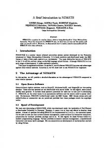
To further improve the finite-time performance of the COMPASS algorithm and make it competitive with commercial DOvS solvers, Xu, Nelson, and Hong (2009) developed an industrial strength COMPASS (ISC) algorithm that takes the COMPASS algorithm as its core, but adds other steps to make the algorithm more efficient in solving practical problems. The ISC algorithm uses a different approach to the tradeoff of exploration, exploitation and estimation. It divides the optimization process into three stages: a global stage that explores the entire feasible region and identifies several regions possibly with competitive locally optimal solutions, a local stage that exploits the local information and finds a locally optimal solution for each of the regions identified in the global stage, and a clean-up stage that selects the best solution among all identified locally optimal solutions and estimates the true value of the selected solution. The ISC algorithm uses a niching genetic
81
Hong and Nelson
Figure 1: ISC approach to the tradeoff of exploration, exploitation and estimation (Xu, Nelson, and Hong 2009).
algorithm for the global stage, the COMPASS algorithm for the local stage, and a R&S procedure for the clean-up stage. It also defines meaningful and testable transition rules between the stages. Figure 4, taken from Xu, Nelson, and Hong (2009), is an illustration of the approach. Xu, Nelson, and Hong (2009) also compared the ISC algorithm with the OptQuest engine, which is the solver used in OptQuest and embedded in many commercial simulation packages, for a number of examples with different characteristics. They found that the ISC algorithm is competitive with OptQuest, despite enforcing finite-sample and asymptotic guarantees. The C++ implementation of the ISC algorithm along with its instructions and related papers are free for downloading from . 5
WORKING WITH COMMERCIAL OVS SOFTWARE
Many simulation products have integrated OvS software. Robust heuristics are the most common algorithms found in such software. In this section, which is based on Chapter 12 in Banks et al. (2005), we provide some guidance on their use. A “robust heuristic” is an OvS procedure that does not depend on strong problem structure to be effective, can be applied to problems with mixed types of decision variables, and is tolerant of some sampling variability. Genetic algorithms and tabu search are two prominent examples, but there are many others and many variations. Such heuristics have been shown empirically to be highly effective on difficult deterministic optimization problems. However, they typically provide no performance guarantees for deterministic problems, much less the stochastic simulation problems considered here. Therefore, we offer three suggestions for using commercial products that employ a robust heuristic to make them more effective: controlling sampling variability, restarting, and clean up. 5.1 Control Sampling Variability In many cases, it will up to the simulation user to determine how many replications will be undertaken at each potential solution. This is a difficult problem in general. Ideally, the number of replications should increase as the heuristic discovers better solutions because it is much more difficult to distinguish solutions that are close in performance from those that differ substantially. At the beginning of the search it may be easy for the heuristic to identify good solutions and search directions, because clearly inferior solutions are being compared to much better ones, but late in the search this might not be the case. If the OvS software has an “adaptive” setting—meaning it adjusts the number of replications based on the variance of the simulation estimates—then use it. If, on the other hand, you must specify a fixed number of replications per solution, then a preliminary experiment should be conducted: Simulate several solutions, some at the extremes of the feasible space and some nearer the center. Compare the apparent best and apparent worst of these solutions, using the tools described earlier. Find the minimum number of replications required to declare them to be statistically significantly different. This is the minimum number of replications that should be used.
82
Hong and Nelson 5.2 Restarting the Optimization Because robust heuristics provide no guarantees that they converge to the optimal solution, it makes sense to run the optimization several times to see which run yields the best solution. Each optimization run should use different random number seeds or streams and should start from different initial solutions. Be sure to start at solutions on the extremes of the solution space, in the center of the space, or even at randomly generated solutions. If people familiar with the system suspect that certain solutions will be good, be sure to include them as starting solutions for the heuristic. Remember that the goal is to find the best solution you can find, so an additional day, or even week, of optimization runs may be well worth it for an important (and perhaps expensive) decision. 5.3 Statistical Clean Up After the optimization run or runs have completed, it is critical to perform a second set of experiments on the top solutions identified by the heuristic to avoid two types of errors: failing to recognize the the best solution that was simulated during the search, and poorly estimating the performance of the solution that is selected at the end. These errors occur because no optimization algorithm can hope to make any progress while at the same time maintaining statistical error control every step of the way, and there is a natural bias toward solutions that, by chance, received favorable simulation samples. Therefore, we recommend “cleaning up” after the search, by which we mean performing a rigorous statistical analysis employing the comparison techniques described in Section 2 to evaluate which are the best or near-best of the solutions discovered during the search. The top 5 to 10% of the solutions simulated during the search should be subjected to this controlled experiment. The “clean up” concept was introduced in Boesel, Nelson, and Kim (2003). 6
CONCLUSIONS
In this article, we give a brief introduction to the recent development of OvS research and practice. As noted in the paper, there is still a large gap between the OvS algorithms developed in the academic research community and the OvS algorithms used in commercial software. The research community likes algorithms with provable statistical guarantees or convergence properties, and the software community mainly uses robust metaheuristics that appear to work but have no such guarantees or properties. Although there has been some interesting recent work trying to bridge the gap, there is still a long way to go. ACKNOWLEDGMENTS The research of the first author is supported in part by the Hong Kong Research Grants Council under the grants CERG 613706 and CERG 613907. REFERENCES Alrefaei, M. H., and S. Andrad´ottir. 1999. A simulated annealing algorithm with constant temperature for discrete stochastic optimization. Management Science 45:748–764. Andrad´ottir, S. 1995. A method for discrete stochastic optimization. Management Science 41:1946–1961. Andrad´ottir, S. 1999. Accelerating the convergence of random search methods for discrete stochastic optimization. ACM Transactions on Modeling and Computer Simulation 9:349–380. Andrad´ottir, S. 2006. Simulation optimization with countably infinite feasible regions: Efficiency and convergence. ACM Transactions on Modeling and Computer Simulation 16:357–374. Banks, J., J. S. Carson, B. L. Nelson and D. Nicol. 2005. Discrete-Event System Simulation. Fourth Edition. Prentice Hall, Inc., Upper Saddle River, NJ. Barton, R. R., and M. Meckesheimer. 2006. Metamodel-based simulation optimization. Chapter 18 in Handbooks in Operations Research and Management Science: Simulation. North-Holland. Batur, D., and S.-H. Kim. 2009. Finding feasible systems in the presence of constrains on multiple performance measures. ACM Transactions on Modeling and Computer Simulation, forthcoming. Bechhofer, R. E. 1954. A single-sample multiple decision procedure for ranking means of normal populations with known variances. Annals of Mathematical Statistics 25:16–39. Boesel, J., B. L. Nelson, and S.-H. Kim. 2003. Using ranking and selection to ‘clean up’ after simulation optimization. Operations Research 51:814-825.
83
Hong and Nelson Borkar, V. S. 2008. Stochastic Approximation: A Dynamic Systems Viewpoint. Cambridge University Press. Branke, J., Chick, S., and Schmidt, C. 2007. Selecting a selection procedure. Management Science 53:1916-1932. Chen, C.-H., J. Lin, E. Y¨ucesan, and S. E. Chick. 2000. Simulation budget allocation for further enhancing the efficiency of ordinal optimization. Discrete Event Dynamic Systems: Theory and Applications 10:251–270. Chick, S. E., and K. Inoue. 2001. New two-stage and sequential procedures for selecting the best simulated system. Operations Research 49:732–743. Fabian, V. 1974. Note on Anderson’s sequential procedures with triangular boundary. Annals of Statistics 2:170–176. Fu, M. C. 2002. Optimization for simulation: Theory vs. practice. INFORMS Journal on Computing 14:192–215. Fu, M. C. 2008. What you should know about simulation and derivatives. Naval Research Logistics 55:723–736. Fu, M. C., and J. Q. Hu. 1997. Conditional Monte Carlo: Gradient Estimation and Optimization Applications, Kluwer Academic Publishers, Norwell, MA. Glynn, P. W. 1990. Likelihood ratio gradient estimation for stochastic systems. Communications of the ACM 33:75–84. Gong, W. B., Y. C. Ho, and W. Zhai. 1999. Stochastic comparison algorithm for discrete optimization with estimation. SIAM Journal on Optimization 10:384–404. Ho, Y. C., and X.-R. Cao. 1983. Optimization and perturbation analysis of queueing networks. Journal of Optimization Theory and Applications 40:559–582. Hong, L. J. 2009. Estimating quantile sensitivities. Operations Research 57: 118–130. Hong, L. J., and G. Liu. 2009. Pathwise estimation of probability sensitivities through terminating and steady-state simulations. Operations Research, forthcoming. Hong, L. J., and B. L. Nelson. 2005. The tradeoff between sampling and switching: New sequential procedures for indifference-zone selection. IIE Transactions 37:623–634. Hong, L. J., and B. L. Nelson. 2006. Discrete Optimization via Simulation using COMPASS. Operations Research 54:115–129. Hong, L. J., and B. L. Nelson. 2007a. A framework for locally convergent random search algorithms for discrete optimization via simulation. ACM Transactions on Modeling and Computer Simulation 17:19/1–19/22. Hong, L. J., and B. L. Nelson. 2007b. Selecting the best system when systems are revealed sequentially. IIE Transactions 39:723–734. Hu, J., M.C. Fu, and S.I. Marcus. 2007. A model reference adaptive search method for global optimization. Operations Research 55:549–568. Kiefer, J., and Wolfowitz, J. 1952. Stochastic Estimation of the Maximum of a Regression Function. Annals of Mathematical Statistics 23:462-466. Kim, S.-H. 2005. Comparison with a standard via fully sequential procedure. ACM Transactions on Modeling and Computer Simulation 15:1–20. Kim, S.-H., and B. L. Nelson. 2001. A fully sequential procedure for indifference-zone selection in simulation. ACM Transactions on Modeling and Computer Simulation 11:251–273. Kim, S.-H., and B. L. Nelson. 2006. On the asymptotic validity of fully sequential selection procedures for steady-state simulation. Operations Research 54:475–488. Kim, S.-H., and B. L. Nelson. 2007. Recent Advances in Ranking and Selection. 2007 Winter Simulation Conference Proceedings, 162-172. Kushner, H. J., and G. Yin. 2003. Stochastic approximation and recursive algorithms and applications, 2nd Edition. Springer. Law, A. M. 2007. Simulation Modeling and Analysis, 4th Edition. McGraw-Hill. Nelson, B. L., and F. J. Matejcik. 1995. Using Common Random Numbers for Indifference-Zone Selection and Multiple Comparisons in Simulation. Management Science 41:1935–1945. Nelson, B. L., J. Swann, D. Goldsman, and W. Song. 2001. Simple procedures for selecting the best simulated system when the number of alternatives is large. Operations Research 49:950–963. Olafsson, S.. 2006. Metaheuristics. Chapter 21 in Handbooks in Operations Research and Management Science: Simulation. North-Holland. Paulson, E. 1964. A sequential procedure for selecting the population with the largest mean from k normal populations. Annals of Mathematical Statistics 35:174–180. Pichitlamken, J., and B. L. Nelson. 2003. A combined procedure for optimization via simulation. ACM Transaction on Modeling and Computer Simulation 13:155–179. Pichitlamken, J., B. L. Nelson, and L. J. Hong. 2006. A sequential procedure for neighborhood selection-of-the-best in optimization via simulation. European Journal of Operational Research 173:283–298. Prudius, A. A., and S. Andrad´ottir. 2006. Balanced explorative and exploitative search with estimation for simulation optimization. Working Paper, School of ISyE, Georgia Tech, Atlanta, GA.
84
Hong and Nelson Reiman, M., and A. Weiss. 1989. Sensitivity analysis for simulations via likelihood ratios. Operations Research 37:830–844. Rinott, Y. 1978. On two-stage selection procedures and related probability-inequalities. Communications in Statistics A7:799–811. Robbins, H., and S. Monro. 1951. A Stochastic Approximation Method. Annals of Mathematical Statistics 22:400–407. ´ Shi, L., and S. Olafsson. 2000. Nested partitions method for stochastic optimization. Methodology and Computing in Applied Probability 2:271–291. Spall, J. C. 1992. Multivariate stochastic approximation using a simultaneous perturbation gradient approximation. IEEE Transactions on Automatic Control 37:332–341. Spall, J. C. 1998. An overview of the simultaneous perturbation method for efficient optimization. Johns Hopkins APL Technical Digest 19:482-492. Xu, J., B. L. Nelson, and L. J. Hong. 2009. Industrial Strength COMPASS: A Comprehensive Algorithm and Software for Optimization via Simulation. ACM Transactions on Modeling and Computer Simulation, forthcoming. Yan, D., and H. Mukai. 1992. Stochastic discrete optimization. SIAM Journal of Control and Optimization 30:594–612. AUTHOR BIOGRAPHIES L. JEFF HONG is an associate professor in the Department of Industrial Engineering and Logistics Management at The Hong Kong University of Science and Technology. His research interests include Monte Carlo method, financial engineering, stochastic optimization. He is currently an associate editor of Operations Research, Naval Research Logistics and ACM Transactions on Modeling and Computer Simulation. BARRY L. NELSON is the Charles Deering McCormick Professor and Chair of the Department of Industrial Engineering and Management Sciences at Northwestern University. His research interests are in the design and analysis of stochastic simulation experiments, and simulation input modeling.
85