Sensors 2013, 13, 13779-13801; doi:10.3390/s131013779 OPEN ACCESS
sensors ISSN 1424-8220 www.mdpi.com/journal/sensors Article
A Buoy for Continuous Monitoring of Suspended Sediment Dynamics Philip Mueller 1,*, Heiko Thoss 1, Lucas Kaempf 2 and Andreas Güntner 1 1
2
Helmholtz Centre Potsdam, German Research Centre for Geosciences, Section 5.4 Hydrology, Telegrafenberg, Potsdam 14473, Germany; E-Mails:
[email protected] (H.T.);
[email protected] (A.G.) Helmholtz Centre Potsdam, German Research Centre for Geosciences, Section 5.2 Climate Dynamics and Landscape Evolution, Telegrafenberg, Potsdam 14473, Germany; E-Mail:
[email protected]
* Author to whom correspondence should be addressed; E-Mail:
[email protected]; Tel.: +49-331-288-1564; Fax: +49-331-288-1570. Received: 29 July 2013; in revised form: 5 September 2013 / Accepted: 25 September 2013 / Published: 14 October 2013
Abstract: Knowledge of Suspended Sediments Dynamics (SSD) across spatial scales is relevant for several fields of hydrology, such as eco-hydrological processes, the operation of hydrotechnical facilities and research on varved lake sediments as geoarchives. Understanding the connectivity of sediment flux between source areas in a catchment and sink areas in lakes or reservoirs is of primary importance to these fields. Lacustrine sediments may serve as a valuable expansion of instrumental hydrological records for flood frequencies and magnitudes, but depositional processes and detrital layer formation in lakes are not yet fully understood. This study presents a novel buoy system designed to continuously measure suspended sediment concentration and relevant boundary conditions at a high spatial and temporal resolution in surface water bodies. The buoy sensors continuously record turbidity as an indirect measure of suspended sediment concentrations, water temperature and electrical conductivity at up to nine different water depths. Acoustic Doppler current meters and profilers measure current velocities along a vertical profile from the water surface to the lake bottom. Meteorological sensors capture the atmospheric boundary conditions as main drivers of lake dynamics. It is the high spatial resolution of multi-point turbidity measurements, the dual-sensor velocity measurements and the temporally synchronous recording of all sensors along the water column that sets the system apart from existing buoy systems. Buoy data collected during a 4-month field
Sensors 2013, 13
13780
campaign in Lake Mondsee demonstrate the potential and effectiveness of the system in monitoring suspended sediment dynamics. Observations were related to stratification and mixing processes in the lake and increased turbidity close to a catchment outlet during flood events. The rugged buoy design assures continuous operation in terms of stability, energy management and sensor logging throughout the study period. We conclude that the buoy is a suitable tool for continuous monitoring of suspended sediment concentrations and general dynamics in fresh water bodies. Keywords: buoy; monitoring; suspended sediments; lake; turbidity; connectivity
1. Introduction Understanding suspended sediment dynamics (SSD) has been an important topic in both applied and process research for several decades. From different perspectives such as hydrology (e.g., [1]), hydraulic engineering (e.g., [2]) and sedimentology (e.g., [3]), scientists have investigated SSD in catchments and in the reservoirs, lakes and estuaries into which the watersheds drain. Duvert et al. [4] pointed out the necessity of monitoring suspended sediments, especially in rural areas that are situated in small mountainous catchments, because these catchments are increasingly facing human pressures due to land use changes. Many recent hydrological studies, therefore, have focused on upland erosion, the resulting reservoir siltation and reduction of reservoir capacity [5,6]. Reservoir siltation can cause a serious reduction in water availability for a given region. Viseras et al. [7] showed that the storage capacity of a reservoir in Spain decreased by around 80% within a 20-year period. Besides reservoir siltation, erosion and sediment transport may also cause a loss of valuable farmland [8] and damage to hydro-electrical facilities [9]. To understand the driving forces and effects of SSD and to develop sustainable mitigation measures, it is necessary to understand the linkage between different landscape units in a catchment that act as source, conveyor and sink for sediments. This linkage is represented by the term ―hydrological connectivity‖. In a hydrological sense, Pringle [10] describes hydrological connectivity as water-mediated transfer of matter, energy and organisms within the hydrological cycle. Due to different spatial scales, scientific backgrounds and perspectives, there exist different sub-definitions of the concept of hydrological connectivity (e.g., see overviews by [11,12]). One of these is the perception of longitudinal connectivity. According to Duvert et al. [12], this stands for sediment behavior between upland and lowland compartments of a landscape and is as yet poorly understood. Intensive monitoring is one way to face this challenge of understanding SSD. There are several studies presenting river catchment SSD monitoring networks at a high spatial and temporal resolution [1]. The tracing of suspended sediments along catchments [3] and the connectivity of SSD in streams to outside-stream compartments like hillslopes and groundwater is a focus of present-day research [12]. A distinct boundary between two spatial compartments is the interface between river catchments and lakes that act as sediment source areas and sediment sinks, respectively. Several studies have touched on this issue of connectivity between catchments and lakes, in particular by
Sensors 2013, 13
13781
investigating reservoir siltation based on remote sensing [7] or source tracing techniques like isotope or magnetic characterization [13]. However, studies that directly link SSD in catchments and reservoirs through monitoring of the spatial and temporal distribution of suspended sediment in both compartments are scarce. Linking the two compartments functionally, Dearing [14] described lake sediments as records of past catchment behavior. Swierczynski et al. [15] presented a 1,600 year chronology of seasonally resolved flood events that was reconstructed from varved lake sediments. Czymzik et al. [16] stressed the importance of flood chronologies from lake sediments as a prolongation of instrumental flood time series. In order to bridge the spatial gap between instrumental catchment data and varved lake sediments, it is also very important to have a good understanding of stratification and mixing processes within the lake. This understanding of intra-lake processes is required to better decipher the past from lacustrine sediment cores [17]. Drifters, satellite remote sensing techniques, conservative tracers and acoustic sensors have the capability to measure flow inside lakes [18–20]. However, only acoustic current meters allow continuous in-situ monitoring of flow velocities. To gain a better understanding of SSD based on long-term and comprehensive observation data, monitoring systems must fulfill the following requirements: Suspended sediment concentrations must be measured continuously at a high spatial and temporal resolution to comply with the expected process dynamics. Given that flood events have a duration of hours to days, depending to the hydrological boundary conditions and catchment characteristics [21], sub-hourly resolution should be the goal. Limno-physical and meteorological boundary conditions acting as forcing parameters for SSD must be measured to resolve, e.g., the effect of mixing and stratification processes. Suspended sediment monitoring in the lake should be consistent with hydro-sedimentological monitoring stations within a catchment in terms of the parameters measured and its temporal resolution to capture the effects of flood-related water and sediment inflow from contributing streams. The system must be able to be deployed and operated at one or more fixed locations within the lake throughout the year. Accessibility, low maintenance effort and flexibility of the system’s structure must be ensured. Buoy-based monitoring systems are potentially a very valuable tool for monitoring sediment dynamics, mixing and stratification directly within water bodies, and thus for establishing the link between catchment processes and lake/reservoir SSD. Buoy systems have, for instance, been developed for studying water quality [22–26]. Alcântara et al. [26] applied the SIMA buoy system to understand turbidity behavior in the Amazonian floodplain and density currents in a Brazilian reservoir. Another example is the Chesapeake Bay Interpretive Buoy System [24], which is a sophisticated system that includes measurement of meteorological parameters, current measurements and point-measurement of water quality parameters and turbidity. The GLUCOS [25] observation system was applied in Lake Michigan to measure dynamics of spring stratification and water quality parameters. The Simpatico system developed by Garel et al. [23] used a YSI buoy system (YSI.com) deployed in a Portuguese estuary in combination with a turbidity measuring multi-parameter probe and two acoustic current sensors.
Sensors 2013, 13
13782
Existing buoy systems presented in the literature, however, do not fully satisfy the needs for exploring processes of SSD in lakes or estuaries as listed above. Systems introduced by e.g., Garel et al. [23] and Alcântara et al. [26] are equipped with single-point turbidity sensor systems and contain no or only single-sensor flow velocity measurements. The limitation of existing systems in particular is the low vertical resolution within the water column, the non-simultaneous measurement in different water depths and the problem of blanking by single-sensor flow velocity measurements. Blanking is the distance from transducers that is required before the sensor is able to obtain valid data. Minimum blanking distance for general purpose Acoustic Doppler Current Profilers is 20–25 cm [27]. In this study we present the design, deployment and initial datasets of a buoy system that meets the above challenges of a lake monitoring system. What sets the system apart from existing buoy systems mainly is: (a) the ability of simultaneous multi-level turbidity, temperature and electrical conductivity measurements; (b) highly resolved flow velocity measurement by two sensors, whereas one sensor is applied for surface and one for flow velocity of the whole water column, which guarantees maximum spatial coverage and resolution; (c) maximum maintainability due to easy accessibility of all sensor units. 2. Monitoring System 2.1. Design of the Buoy The buoy design is focused on system flexibility in the sense of easy extension or modification of the sensor configuration and easy maintenance in terms of accessibility and frequency. The buoy consists of a main body (see Figure 1a), a mast (see Figure 1a) as carrier for the solar panels (see Figure 1c), the mounting for the meteorological sensor unit (see Figure 1c) and the navigation light (see Figure 1c). The body of the buoy serves as enclosure for the battery pack and the logger, as fixture for the measurement chain and as a lifting body. The buoyancy of the lifting body amounts to one cubic meter. The cylindrical shape of the main body (MB) with its large top face area and comparatively small height was chosen to have enough interior space for technical equipment and easy accessibility for maintenance purposes, as well as low pitch and roll behavior and sufficient buoyancy in operation mode. Easy accessibility from a small boat was the main reason for the position of the two openings on the top face of the MB. As shown in Figure 1, the first tray (see Figure 1a) allows access to the batteries, and the second tray (see Figure 1a) to the data logger and communication equipment. The MB provides two places for acoustic current sensors. The integrated cylindrical cavity on the top side (see Figure 1c) next to the mast holds an Acoustic Doppler Current Profiler (ADCP). A special bracket was constructed (see Figure 1b) that assures easy accessibility and maintenance of the ADCP. To hold an Acoustic Doppler Current Meter (ADCM) in place, a clamp-like mounting device (see Figure 1c) exists at the lateral area of the cylindrical MB. Tourism in the region of the deployment area was the main driver for defining the outer appearance of the buoy. It is a compromise between reduced perceptibility in contrast to the surrounding environment and a clear visibility of the buoy for shipping traffic (see Figure 2). Therefore, the MB is kept silver and the mast painted yellow. Buoy visibility at night and in poor weather conditions is assured by a programmable navigation light.
Sensors 2013, 13
13783
Figure 1. Technical drawing of the buoy. (a) The side view, (b,c) The top view of the main body and the entire buoy. The measurement chain is not illustrated. It is attached to the center of the bottom side of the main body.
(a)
(b)
(c)
Figure 2. Buoy in operation and plate anchor as used for the mooring.
Sensors 2013, 13
13784
2.2. Energy Supply and Mooring The energy supply system (ESS) of the buoy consists of a battery module, a solar charge controller and four solar panels. The battery module is made of four bridged 33 Ampere hour batteries. The bridged connection of the four batteries leads to a total energy storage capacity of 132 Amperes. The batteries are charged by four solar panels (Solara S160M136) with 45 Wp each. With the umbrella-like construction of the mounting plates at the mast (see Figure 1), the solar panels can be folded out up to an angle of 90 degrees. This makes them adjustable to different altitudes of the sun throughout the year to reach a maximum energy yield. Charging of batteries and preventing exhaustive discharge is managed by a Phocos PL20 solar charge controller. The technical setup of the ESS guarantees an efficient balance of charge and discharge of the batteries. Assuming low energy input due to poor weather conditions and a maximum power consumption of 13.8 Ampere hours per day (Ah/d) at 12 V, the system enables a minimum redundancy of 7 days. The logging unit has an energy load of 0.5 Ah/d, the sensors 11.4 Ah/d and the navigation light 1.9 Ah/d. The mooring of every buoy is composed of three plate anchors made by Uwitec (see Figure 2). Plate anchors were chosen because of the very fine sediments in the deployment area (Lake Mondsee) with a mostly fine sandy to coarse silty texture [15]. Three mooring line handlers are evenly distributed around the MB of the buoy as can be seen in Figures 1 and 2. The number of tie points prevents a twisting around the vertical axis of the buoy. Based on previous experience with the mooring of drilling platforms, the length of the mooring lines is three times the water depth at the buoy position. 2.3. Sensor Equipment, Data Logging and Communication The sensor equipment of the buoy consists of three main units (water quality, current and climate, see Table 1). Table 1. Measured parameters of the buoy system. Water Quality Parameter [Unit]
Current Parameter [Unit]
Turbidity [NTU] Water Temperature [°C] Electrical Conductivity [mS/m]
Flow Speed [mm/s] Flow Direction [deg/10]
Meteorology Parameter [Unit] Relative Humidity [%] Air Temperature [°C] Wind Speed [m/s] Wind Direction [deg]
As an indirect measure of suspended sediment concentrations, turbidity is continuously and simultaneously recorded at nine different water depths to reach a high vertical resolution across the water column with a depth of about 23 m in the test deployment. Nine Forest Technology Systems, Inc. (FTS) (http://www.ftsenvironmental.com) nephelometric turbidity sensors were distributed along the measurement chain. Table 2 presents detailed information regarding the sensor distribution. The FTS-sensors have wipers as cleaning systems that prevent the optical face of the sensor from fouling by cleaning it every 15 min. According to the manufacturer, the DTS-12 uses true nephelometric geometry, which improves the signal-to-noise ratio by measuring the forward and backscattered light
Sensors 2013, 13
13785
at 90°angle to the light beam. In order to guarantee extreme accuracy the built-in microprocessor takes 100 readings over 5 s and then computes and outputs turbidity values (accuracy and range see Table 3). An Uwitec Water Sampler (www.uwitec.at) is used to collect water samples at every depth in order to calibrate the turbidity sensors against suspended sediment concentrations from the water samples based on a linear regression [28]. Besides turbidity, the FTS DTS-12 sensors also measure water temperature. To assure a certain redundancy in water temperature measurements and to collect data on electrical conductivity as a proxy for total dissolved solids, and potentially for water density changes and suspended sediment concentrations, Campbell Scientific, Inc. (CS, http://www.campbellsci.com) CS547A-L electrical conductivity and temperature sensors were added to the measurement chain at similar depths as the turbidity sensors (Table 2). The measurement chain is fixed at the centre underneath the MB of the buoy. An anchor rope with a diameter of 10 mm is the backbone of the chain to which the single sensors are fixed. The top end of the chain is equipped with a leader for easy handling and recovery of the chain or of single sensors, and to the bottom end a sinker was fixed to keep the chain taut. Retrieving information on flow conditions at a high spatial resolution is crucial for understanding the limno-physical boundary conditions, e.g., flow paths, currents, and thus the resulting sediment distribution inside the water body. Near-surface flow speed and direction are measured by a Nortek (http://www.nortek-as.com) Aquadopp Current Meter (ADCM) with a 2 MHz frequency and a 0.75 m measurement cell size in a water depth of 0.3 m (see Table 2 for detailed specifications), resulting in an integral signal from 0.3–1.05 m water depth. A Nortek Aquadopp Profiler (ADCP) is used to record these parameters in a profile from 1.5 m below lake level to the bottom of the lake with a cell size of 2 m. ADCM and ADCP follow the same principles of measurement based on three acoustic beams. The only difference is that the ADCP records an integral signal of flow velocity and flow direction for every depth increment, while the ADCM measures this signal for every single beam in one depth. An ADCP is used to determine current velocities by using the Doppler shift of a backscattered acoustic signal [29]. The choice of the acoustic frequency of the ADCP reflects a compromise between the desired vertical resolution and the water depth at the site. On the one hand, a higher operation frequency leads to smaller cell sizes and higher vertical resolution, and on the other hand, to a lower depth range of the ADCP. In the present configuration, the ADCP operates at a frequency of 400 kHz. This sensor offers a profiling range of 60 to 90 m and a cell size of 2–8 m. For the test deployment, a 2 m cell size was chosen. The frequency of 2 MHz of the ADCM is a default by the manufacturer.
Sensors 2013, 13
13786
Table 2. Allocation and technical overview of sensors attached to buoy during test operation. Logging interval for all sensors is ∂t = 15 min. Type of Sensor FTS DTS-12 (Nephelometric turbidity sensor)
CS547 A-L
Nortek Aquadopp Current Meter (acoustic Doppler current meter at 2 MHz)
Nortek Aquadopp Profiler (acoustic Doppler current profiler at 400 kHz)
RM Young Wind Monitor
UMS TempRH
Parameter [Range/Accuracy] Turbidity [0–1600 NTU (nominal)/±2% of reading (0–399 NTU), ±4% of reading (400–1,600 NTU)] and water temperature[0 °C–40 °C/±0.2 °C] Electrical conductivity [approx. 0.005–7.0 mScm−1/±5% of reading 0.44 to 7.0 mScm−1and ±10% of reading 0.005–0.44 mScm−1 for standard solutions] and water temperature [0 °C–50 °C/±0.4 °C] Flow speed [±5 ms−1/1% of measured value ±0.5 cms−1]and flow direction [Azimuth: 360°/2°/resp. 0.1°for tilt