A Collection-Distribution Center Location and Allocation Optimization ...

Hindawi Mathematical Problems in Engineering Volume 2017, Article ID 7863202, 15 pages https://doi.org/10.1155/2017/7863202

Research Article A Collection-Distribution Center Location and Allocation Optimization Model in Closed-Loop Supply Chain for Chinese Beer Industry Kai Kang, Xiaoyu Wang, and Yanfang Ma School of Economics and Management, Hebei University of Technology, Tianjin 300401, China Correspondence should be addressed to Yanfang Ma; [email protected] Received 13 October 2016; Revised 4 March 2017; Accepted 9 March 2017; Published 1 May 2017 Academic Editor: Shuming Wang Copyright © 2017 Kai Kang et al. This is an open access article distributed under the Creative Commons Attribution License, which permits unrestricted use, distribution, and reproduction in any medium, provided the original work is properly cited. Recycling waste products is an environmental-friendly activity that can result in manufacturing cost saving and economic efficiency improving. In the beer industry, recycling bottles can reduce manufacturing cost and the industry’s carbon footprint. This paper presents a model for a collection-distribution center location and allocation problem in a closed-loop supply chain for the beer industry under a fuzzy random environment, in which the objectives are to minimize total costs and transportation pollution. Both random and fuzzy uncertainties, for which return rate and disposal rate are considered fuzzy random variables, are jointly handled in this paper to ensure a more practical problem solution. A heuristic algorithm based on priority-based global-local-neighbor particle swarm optimization (pb-glnPSO) is applied to ensure reliable solutions for this NP-hard problem. A beer company case study is given to illustrate the application of the proposed model and to demonstrate the priority-based global-local-neighbor particle swarm optimization.

1. Introduction Due to resource scarcity and environmental concerns, responsible companies are beginning to pay attention to the future of the planet and the global environment. Recycling used products for remanufacturing is, therefore, becoming of greater importance in supply chain management, a move that can dramatically reduce carbon emissions [1]. Closedloop supply chain (CLSC) combines the forward supply chain with a reverse supply chain to cover the whole product life cycle [2], with the manufacturing of new products and the transportation to customers via distribution centers and retailers as the forward supply chain and recycling, sorting, disposal, and remanufacturing as the reverse supply chain. In recent years, the CLSC has received a great deal of academic and business attention because of the need to be socially responsible, global environmental concerns, and government legislation [3, 4], all of which have motivated companies to pay more attention to recycling to reduce costs and lessen their carbon footprint. Facility location and allocation problems (FLAPs) have been widely studied. Subramanian et al. [5] developed

priority-based simulated annealing to solve a CLSC network design problem, in which the distribution center (DC) and the centralized return collection center (CC) were set. Amin and Zhang [6] presented facilities location model for manufacturing and remanufacturing plants and CLSC collection centers, which included demand and return uncertainties. Subulan et al. [7] developed a CLSC network design model for the lead/acid battery industry that considered both financial and collection objectives. CLSC network design in a competitive environment with price-dependent demand was examined by Rezapour et al. [4], in which the DC and CC were separately built. Zeballos et al. [8] proposed a model for a multiperiod CLSC design and planning problem with demand uncertainty that had ten echelons in which the DC and CC were considered. Wang et al. [9] developed a granular robust model for a two-stage waste-to-energy feedstock flow planning problem with uncertain capacity expansion costs. Tokhmehchi et al. [10] developed a hybrid approach to solve a closed-loop supply chain location and allocation problem that considered the minimization of total cost. Vahdani and Mohammadi [11] proposed capacitated bidirectional facilities for CLSC conduct distribution, in

2 which a multipriority queuing system was studied. As a growing number of companies are now engaging in recycling activities due to economic and environmental concerns, distribution and collection activities using the same vehicle have been found to reduce carbon emissions and transportation costs as empty loads can be avoided. In this paper, to benefit company operation and reduce construction costs, a distribution center (DC) is combined with a collection center (CC) into a collection-distribution center (CDC). In practice, as the recycled product owners are usually at the same location as the potential new product buyer [12], a DC/CC combination has lower construction and operating expenses and can significantly reduce environmental pollution. Ramkumar et al. [13] developed a multiechelon, multiperiod, multiproduct closed-loop supply chain network model which was solved using a genetic algorithm with fixed variables. Kaya and Urek [12] presented a facility locationinventory-pricing model without uncertainty to determine optimal facilities locations. Barz [14] proposed an optimization model for a two-stage capacitated facility location and allocation problem with additive manufacturing, in which all variables were certain. Jindal and Sangwan [15] developed a multiobjective model for a CLSC network design problem with the economic and environmental factors being fuzzy uncertain variable and the DC and CC were separate. Ramezani et al. [16] conducted research into a CLSC network design problem that only considered of fuzzy variables. In recent years, uncertainty has attracted more research attention [17–19]. Stochastic programing, robust optimization, and fuzzy set theory have been used to present uncertainty in FLAPs [20, 21]. Wang et al. [22] used prediction sets to solve an expansion planning problem for waste-to-energy (WtE) systems facing future waste supply uncertainty. Keyvanshokooh et al. [23] proposed a novel hybrid robust-stochastic programing (HRSP) approach to simultaneously model two different types of uncertainties by using stochastic scenarios for the transportation costs and polyhedral uncertainty sets for the demand and returns. However, the DC and the CC were separate and the collection disposal rate was a certain variable. Uncertainties exist in both forward and reverse supply chains. However, the uncertainties in the reverse flow are higher than in the forward supply chain [7, 24, 25] as returned product quantity is generally seen as uncertain [23, 26]. Subjective uncertainties such as the decision maker’s choices and environmental coefficients can be dealt with using fuzziness, while objective uncertainties such as unit transportation costs, product prices, and the quantity of unusable products can be dealt with using randomness. In this paper, to reflect the study problem, the return rate and disposal rate are considered fuzzy random variables, which are concurrently handled using triangular fuzzy numbers [7]. Based on the above, a model is formulated to determine the optimum CDC number and location and the allocation strategies for the different facility types. As facilities location and allocation problems are seen as nonconvex, nondifferentiable, strongly NP-hard problems, a collection and distribution center location and allocation problem (CDCLAP) in a closed-loop supply chain under

Mathematical Problems in Engineering a fuzzy random environment is even more complicated. Several different methods have been used to solve NP-hard problems [27–29]. While particle swarm optimization (PSO) has been found to be generally effective [30–32], when the local optimal solution is found, the particle behavior in a basic PSO is directly influenced and therefore frequently falls into a local optimum [33–35]. Because of this problem, several advanced PSOs have been developed to more accurately solve supply chain management problems. Ai and Kachitvichyanukul [36] proposed a global-local-neighbor PSO which was found to be more effective. Based on this innovation, Xu et al. [33] proposed a fuzzy random simulation-based bilevel globallocal-neighbor particle swarm optimization (frs-bglnPSO). In this paper, a priority-based global-local-neighbor particle swarm optimization (pb-glnPSO) is applied to solve the CDCLAP. In summary, this paper proposes a mathematical model to solve a collection-distribution center location and allocation problem in a closed-loop supply chain that considers economic and environmental factors and includes fuzzy random variables for return and disposal rates. The remainder of this paper is organized as follows. Section 2 presents the problem statement and model assumptions, after which a description of the model and its formulations is given in Section 3. The proposed hybrid solution based on the developed pb-glnPSO is described in Section 4 and case study is presented in Section 5 to illustrate model formulation and the proposed method. Finally, Section 6 gives conclusions and indications for future research extensions.

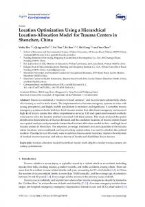
2. Research Problem Statement In this paper, a company with factories in certain locations and retailers in different customer zones is considered. The company needs to decide the locations for their integrated collection and distribution centers (CDCs), at which both a used product collection network and a new product distribution network are to be jointly [12]. As CDCs reduce construction and transportation costs because the same vehicles are used for both distribution and recycling, in this paper, only CDCs are considered. A general illustration of the classical CDCLAP for a closed-loop supply chain is shown in Figure 1, with the CLSC framework shown in Loop 1. The CLSC framework has four echelons: factories, CDCs, retailers, and disposal centers [11]. The forward supply chain begins with new production, after which the finished products are transported from the factories to the retailers via the CDCs. In the reverse supply chain, returned products are collected and transported to the CDCs, where the recycled products are inspected, consolidated, and sorted into those that are available for remanufacturing, which are sent to the factories, and those that are unsuitable for remanufacturing, which are transported to the disposal centers [23]. A CDC supplies products to multiple retailers; however, retailer demand is fulfilled by only one production site. A CDC can also handle products from different factories and dispatch returned products to multiple factories for remanufacturing.

Mathematical Problems in Engineering

3

Factory 1

Factory 2

Retailer 1

Collection-distribution center 1 Retailer 2

Loop 1

Disposal center

Retailer 3

Factory 3

Collection-distribution center 2 Factory 4

Retailer 4

Figure 1: The closed-loop supply chain network.

In the CLSC examined in this paper, the retailers’ demand is estimated based on preorders. However, the return rate is considered to be a fuzzy random variable as customers may not return the used product or the product may be broken. Consequently, the availability of recycled products is unsure because of unsure transportation and carrying losses. Another fuzzy random variable considered in this paper is the returned product disposal rate, which is dependent on the inspection and consolidation at the CDC. The assumptions for the proposed problem investigation are as follows: (1) only one product in one period is considered; (2) all alternative CDC locations have been identified; (3) recycling a used product costs less than manufacturing a new one; (4) the CDCs and factories have capacity limits [37– 39]. As considering incapacitated facilities is an unrealistic assumption in many LAPs, many researchers have assigned a maximum capacity level to facilities to model more realistic decisions; (5) the factories’, retailers’, and disposal centers’ locations are known; (6) new product and returned product storage are allowed at the CDCs [21]. The initial problem is deciding which CDCs to select from the candidate sites and which allocation strategies to select to minimize total CDC costs: operating costs, transportation costs, and transportation pollution costs, while also considering flow constraints, capacity limits, and retailer demand.

3. Modelling In this section, the mathematical formulations are given for the CDCLAP in the CLSC and the notations are given in the Notations to facilitate the problem description. 3.1. Objective Functions. Based on the variables mentioned in the Notations, the objectives are to minimize total costs

and to minimize the environmental effects with the primary objective being minimizing total cost. 3.1.1. Economic Objective. In general, decision makers seek to minimize total costs, which are made up of transportation costs, fixed costs, and operating costs. The minimization objective can be described as min 𝐹1 𝐼

𝐽

𝐼

𝐾

𝑝 𝑑 = ∑ ∑𝐶𝑖𝑗 𝑃𝑗𝑖 + ∑ ∑ 𝐶𝑖𝑘 𝑄𝑖𝑘 (1 + 𝑎̃𝑘 ) 𝑖=1 𝑗=1 𝐼

𝑖=1 𝑘=1

𝑁

𝐾

𝑤̃ ̃ + ∑ ∑ ∑ 𝐶𝑖𝑛 𝑏𝑖 𝑎𝑘 𝑄𝑖𝑘

(1)

𝑖=1 𝑛=1 𝑘=1 𝐼

𝐽

𝐾

𝐼

𝑁

𝑝 ̃ + ∑ ∑ ∑ ∑ 𝐶𝑖𝑗 𝑎̃𝑘 𝑄𝑖𝑘 (1 − 𝑏𝑖 ) + ∑𝐹𝑖𝑐 𝑋𝑖 𝑖=1 𝑗=1 𝑘=1 𝑛=1 𝐼

𝐽

𝑖=1

𝐼

𝐾

+ ∑ ∑ 𝑉𝑖𝑐 𝑃𝑗𝑖 + ∑ ∑ RV𝑐𝑖 𝑎̃𝑘 . 𝑖=1 𝑗=1

𝑖=1 𝑘=1

Equation (1) calculates the total cost, in which 𝑝 ∑𝐼𝑖=1 ∑𝐽𝑗=1 𝐶𝑖𝑗 𝑃𝑗𝑖 is the new product transport costs from 𝑑 ̃ the factories to the CDC, ∑𝐼𝑖=1 ∑𝐾 𝑘=1 𝐶𝑖𝑘 𝑄𝑖𝑘 (1 + 𝑎𝑘 ) is the transport costs between the CDCs and the retailers, and 𝐾 𝑤̃ ̃ ∑𝐼𝑖=1 ∑𝑁 𝑛=1 ∑𝑘=1 𝐶𝑖𝑛 𝑏𝑖 𝑎𝑘 𝑄𝑖𝑘 is the returned product delivery costs from the CDCs to the disposal centers. The returned product transportation costs from the CDCs to disposal 𝑝 ̃ centers are measured as ∑𝐼 ∑𝑁 ∑𝐾 ∑𝑁 𝐶 𝑎̃ 𝑄 (1 − 𝑏 ). 𝑖=1

𝑛=1

𝑘=1

𝑛=1

𝑖𝑗 𝑘

𝑖𝑘

𝑖

The fixed costs for opening a new CDC are ∑𝐼𝑖=1 𝐹𝑖𝑐 𝑋𝑖 . ∑𝐼𝑖=1 ∑𝐽𝑗=1 𝑉𝑖𝑐 𝑃𝑗𝑖 denotes the new product variable costs.

4

Mathematical Problems in Engineering

𝑐̃ ∑𝐼𝑖=1 ∑𝐾 𝑘=1 RV𝑖 𝑎𝑘 calculates the returned product operating costs. As it is very difficult to handle objective functions with fuzzy random factors, Kruse and Meyer [40] demonstrated that the fuzzy expected value could be represented by a single fuzzy number. Based on the theory proposed by Heilpern [41], without a loss of generality, the expected value operator is used to convert the uncertain model into a deterministic model, which can then be used to transform the fuzzy random objective functions into their crisp equivalences, as shown in

min 𝐹1 =

𝐼

𝐽

𝑝 ∑ ∑𝐶𝑖𝑗 𝑃𝑗𝑖 𝑖=1 𝑗=1 𝐼

𝑁

+

𝐾

𝐼

(1 + EV [𝑎̃𝑘 ])

𝑑 𝑄𝑖𝑘 ∑ ∑ 𝐶𝑖𝑘 𝑖=1 𝑘=1

𝐾

̃ 𝑤 + ∑ ∑ ∑ 𝐶𝑖𝑛 EV [𝑏𝑖 ] EV [𝑎̃𝑘 ] 𝑄𝑖𝑘

(2)

𝑖=1 𝑛=1 𝑘=1 𝐼

𝐽

𝐾

𝑁

𝑝 ̃ + ∑ ∑ ∑ ∑ 𝐶𝑖𝑗 EV [𝑎̃𝑘 ] 𝑄𝑖𝑘 (1 − EV [𝑏𝑖 ]) 𝐽

𝐼

𝐼

𝑖=1 𝑗=1

𝐾

𝐾

= ∑ ∑𝛽𝑖𝑗 𝑃𝑗𝑖 + ∑ ∑ 𝛽𝑖𝑘 𝑄𝑖𝑘 (1 + EV [𝑎̃𝑘 ]) 𝑖=1 𝑗=1 𝐼

𝑖=1 𝑘=1

𝑁

𝐾

𝐼

𝐾

𝑁

𝑖=1 𝑗=1 𝑘=1 𝑛=1

∑𝐼𝑖=1 ∑𝐽𝑗=1 𝛽𝑖𝑗 𝑃𝑗𝑖 is the environmental pollution caused by the transportation activities from the factories to the ̃ CDCs. ∑𝐼𝑖=1 ∑𝐾 𝑘=1 𝛽𝑖𝑘 𝑄𝑖𝑘 (1 + EV[𝑎𝑘 ]) is the summation of the carbon footprints for transporting products between the ̃ CDCs and retailers. ∑𝐼 ∑𝑁 ∑𝐾 𝛽 EV[𝑏 ]EV[𝑎̃ ]𝑄 is 𝑛=1

𝑘=1

𝑖𝑛

𝑖

(4)

𝑁

(5)

≤ ∑𝛾𝑗 . 𝑗=1

𝐷𝑘 is the demand from retailer 𝑘 and 𝛾𝑗 is the capacity of 𝑝 ̃ factory 𝑗. ∑𝐼 ∑𝐾 ∑𝑁 𝐶 EV[𝑎̃ ]𝑄 (1 − EV[𝑏 ]) calculates 𝑖=1

𝑘=1

𝑛=1

𝑘

𝑖𝑗

𝑖𝑘

𝑖

the returned product quantity transported to factory 𝑗 for remanufacturing. All products for the retailers are processed through the CDCs. The recycled product quantity is always less than the product quantity transported from the factory to the CDC, which can be described as follows: 𝐽

𝐾

𝑗=1

𝑘=1

∑ 𝑃𝑗𝑖 ≥ ∑ EV [𝑎̃𝑘 ] 𝑄𝑖𝑘 .

𝐼

𝐾

𝑖=1

𝑘=1

∑𝑄𝑖𝑘 ≥ ∑ 𝐷𝑘 .

̃ + ∑ ∑ ∑ ∑ 𝛽𝑖𝑗 EV [𝑎̃𝑘 ] 𝑄𝑖𝑘 (1 − EV [𝑏𝑖 ]) .

𝑖=1

𝐾

𝑖=1 𝑘=1 𝑛=1

𝑖=1 𝑛=1 𝑘=1 𝐽

∀𝑖 ∈ Ω.

𝑎̃𝑘𝑖 is a fuzzy random variable indicating the used product return rate transported from the retailer 𝑘 to CDC 𝑖. 𝑄𝑖𝑘 indicates the product quantity from CDC 𝑖 to retailer 𝑘. 𝑃𝑗𝑖 indicates the product quantity transported from factory 𝑗 to CDC 𝑖. 𝛼𝑖 is the capacity of CDC 𝑖. Within the capacity constraint, the factory is able to manufacture new products to meet retailer needs as well as deal with the returned products from the CDCs.

(3)

̃ + ∑ ∑ ∑ 𝛽𝑖𝑛 EV [𝑏𝑖 ] EV [𝑎̃𝑘 ] 𝑄𝑖𝑘 𝐼

𝑗=1

(6)

𝑃𝑗𝑖 is a variable indicating the new product quantity transported from factory 𝑗 to CDC 𝑖. 𝑎̃𝑘 𝑄𝑖𝑘 refers to the returned product quantity transported from retailer 𝑘 to CDC 𝑖. The products provided to the retailers should meet their demand.

min 𝐹2 𝐼

𝑘=1

𝐽

𝑖=1 𝑘=1

3.1.2. Environmental Objective. The secondary objective is to minimize the transportation carbon emissions associated with the CLSC operations, an area that has attracted significant recent research attention [42]. The following expression represents the transportation carbon emissions between the CDCs and the factories, the CDCs and the retailers, and the CDCs and the disposal centers.

𝐽

𝐽

𝑘=1

̃ Note that EV[𝑎̃𝑘 ] or EV[𝑏𝑖 ] above represents two expected values: the first is used to convert the fuzzy random variables into fuzzy numbers based on Kruse and Meyer’s 1987 theory, and the second is used to transform the fuzzy numbers into deterministic numbers based on Heilpern’s 1992 theory.

𝐼

𝐾

∑ EV [𝑎̃𝑘 ] 𝑄𝑖𝑘 + ∑𝑃𝑗𝑖 ≤ 𝛼𝑖

𝐾

+ ∑𝐹𝑖𝑐 𝑋𝑖 + ∑ ∑𝑉𝑖𝑐 𝑃𝑗𝑖 + ∑ ∑ RV𝑐𝑖 EV [𝑎̃𝑘 ] . 𝑖=1

3.2. Constraints. Note that as each CDC has its own capacity limit, it is unable to service goods beyond capacity; therefore, the capacity limit restriction can be written as follows:

𝑝 ̃ ∑ 𝐷𝑘 + ∑ ∑ ∑ 𝐶𝑖𝑗 EV [𝑎̃𝑘 ] 𝑄𝑖𝑘 (1 − EV [𝑏𝑖 ])

𝑖=1 𝑗=1 𝑘=1 𝑛=1 𝐼

the total carbon footprint from the CDCs to the disposal ̃ 𝐾 𝑁 ̃ centers, and ∑𝐼𝑖=1 ∑𝑁 𝑛=1 ∑𝑘=1 ∑𝑛=1 𝛽𝑖𝑗 EV[𝑎𝑘 ]𝑄𝑖𝑘 (1 − EV[𝑏𝑖 ]) is the carbon footprint from the CDCs to factories for returned products.

𝑘

𝑖𝑘

(7)

𝑄𝑖𝑘 is the product quantity CDC 𝑖 sends to retailer 𝑘. The stochastic variable 𝐷𝑘 is the retailer 𝑘’s demand based on order quantity. The returned product quantity transported to the CDCs is more than the product quantity transported to disposal centers. 𝐾

𝑁

𝐾

̃ ∑ EV [𝑎̃𝑘 ] 𝑄𝑖𝑘 ≥ ∑ ∑ EV [𝑏𝑖 ] EV [𝑎̃𝑘 ] 𝑄𝑖𝑘 .

𝑘=1

𝑛=1 𝑘=1

(8)

Mathematical Problems in Engineering

5

EV[𝑎̃𝑘 ]𝑄𝑖𝑘 is the expression for the returned product quantity ̃ from retailer 𝑘 to CDC 𝑖, and EV[𝑏𝑖 ]EV[𝑎̃𝑘 ]𝑄𝑖𝑘 is the product quantity transported from CDC 𝑖 to retailer 𝑘. There should be at least one CDC and there should be no more CDCs than the specified upper limit.

𝐼

𝑖=1

𝑖=1 𝑗=1

𝐽

𝐼

𝐼

𝑖=1 𝑗=1

(9)

𝑖=1 𝑘=1

𝐾

𝐼

𝑖=1 𝑘=1

𝐾

𝑁

̃ + ∑ ∑ ∑ 𝛽𝑖𝑛 EV [𝑏𝑖 ] EV [𝑎̃𝑘 ] 𝑄𝑖𝑘

𝐼

𝑖=1 𝑛=1 𝑘=1

(10)

𝑖=1

𝐽

𝐼

𝑈 is the upper limit for the number of CDCs, which is dependent on demand, returned product quantity, and fixed capacity constraints. Each retailer must be serviced by only one CDC.

𝐾

𝑁

̃ + ∑ ∑ ∑ ∑ 𝛽𝑖𝑗 EV [𝑎̃𝑘 ] 𝑄𝑖𝑘 (1 − EV [𝑏𝑖 ]) 𝑖=1 𝑗=1 𝑘=1 𝑛=1

s.t.

𝐾

𝐽

𝑘=1

𝑗=1

∑ EV [𝑎̃𝑘 ] 𝑄𝑖𝑘 + ∑𝑃𝑗𝑖 ≤ 𝛼𝑖 𝑥𝑖

𝐼

∑𝑦𝑖𝑘 = 1.

𝐾

Since 𝑥𝑖 and 𝑦𝑖𝑘 are binary variables, the following constraints are required:

𝑦𝑖𝑘 = {0, 1} , ∀𝑖 ∈ Ω, ∀𝑘 ∈ Φ.

∀𝑖 ∈ Ω ∀𝑗 ∈ Ψ ∀𝑘 ∈ Φ

(11)

𝑖=1

𝑥𝑖 = {0, 1} , ∀𝑖 ∈ Ω,

𝐾

= ∑ ∑𝛽𝑖𝑗 𝑃𝑗𝑖 + ∑ ∑ 𝛽𝑖𝑘 𝑄𝑖𝑘 (1 + EV [𝑎̃𝑘 ])

𝑖=1

∑𝑥𝑖 ≤ 𝑈.

𝐼

min 𝐹2

𝐼

1 ≤ ∑𝑥𝑖 ,

𝐽

𝐼

+ ∑𝐹𝑖𝑐 𝑋𝑖 + ∑ ∑𝑉𝑖𝑐 𝑃𝑗𝑖 + ∑ ∑ RV𝑐𝑖 EV [𝑎̃𝑘 ]

𝐼

𝑖=1 𝑘=1 𝑛=1

𝑘=1

𝐽

(12)

𝑥𝑖 is a binary variable indicating whether a CDC is opened at point 𝑖. If location 𝑖 is chosen to open a CDC, then 𝑥𝑖 ; otherwise, 𝑥𝑖 = 0. 𝑦𝑖𝑘 is a binary variable indicating whether retailer 𝑘 is serviced by CDC 𝑖. If 𝑦𝑖𝑘 = 1, then retailer 𝑘 is serviced by CDC 𝑖; otherwise, 𝑦𝑖𝑘 = 0. 3.3. Global Model. From the formulation above, the model for the CDCLAP with capacity, flow, and quantity constraints is developed with the aims of minimizing total costs and total transportation pollution with the primary objective of minimizing the total cost. In the CLSC, both new and returned products are considered. The product can be reproduced to save raw materials and reduce waste and pollution. In our model, all costs involved in the CDCLAP are considered as well as the influence of the transportation activity pollution. Fuzzy random theory is used to deal with the real world complex uncertainties and ensure more scientific decisions. Therefore, this CDC situation is closer to the real situation as it can deal with complicated practical problems. Finally, the global model is given:

𝑁

𝐾

𝑝 ̃ ∑ 𝐷𝑘 + ∑ ∑ ∑ 𝐶𝑖𝑗 EV [𝑎̃𝑘 ] 𝑄𝑖𝑘 (1 − EV [𝑏𝑖 ])

≤ ∑ 𝛾𝑗

∀𝑗 ∈ Ψ ∀𝑘 ∈ Φ ∀𝑛 ∈ Υ

𝑗=1

𝐽

𝐾

𝑗=1

𝑘=1

∑ 𝑃𝑗𝑖 ≥ ∑ EV [𝑎̃𝑘 ] 𝐾

𝑁

∀𝑖 ∈ Ω ∀𝑗 ∈ Ψ ∀𝑘 ∈ Φ 𝐾

̃ ∑ EV [𝑎̃𝑘 ] 𝑄𝑖𝑘 ≥ ∑ ∑ EV [𝑏𝑖 ] EV [𝑎̃𝑘 ] 𝑄𝑖𝑘 𝑛=1 𝑘=1

𝑘=1

∀𝑖 ∈ Ω ∀𝑘 ∈ Φ ∀𝑛 ∈ Υ 𝐼

𝐾

𝑖=1

𝑘=1

∑𝑄𝑖𝑘 ≥ ∑ 𝐷𝑘 𝐼

1 ≤ ∑𝑥𝑖

∀𝑖 ∈ Ω ∀𝑘 ∈ Φ

∀𝑖 ∈ Ω

𝑖=1

𝐼

∑𝑥𝑖 ≤ 𝑈

∀𝑖 ∈ Ω

𝑖=1

𝑦𝑖𝑘 ≤ 𝑥𝑖

∀𝑖 ∈ Ω, ∀𝑘 ∈ Φ

𝐼

∑𝑦𝑖𝑘 = 1

∀𝑖 ∈ Ω ∀𝑘 ∈ Φ

𝑖=1

min 𝐹1 𝐼

𝐽

𝐼

𝐾

𝑝 𝑑 = ∑ ∑𝐶𝑖𝑗 𝑃𝑗𝑖 + ∑ ∑ 𝐶𝑖𝑘 𝑄𝑖𝑘 (1 + EV [𝑎̃𝑘 ]) 𝑖=1 𝑗=1 𝐼

𝑖=1 𝑘=1

𝑁

𝑖=1 𝑛=1 𝑘=1 𝐽

𝑦𝑖𝑘 = {0, 1}

∀𝑖 ∈ Ω ∀𝑖 ∈ Ω, ∀𝑘 ∈ Φ.

(13)

𝐾

̃ 𝑤 + ∑ ∑ ∑ 𝐶𝑖𝑛 EV [𝑏𝑖 ] EV [𝑎̃𝑘 ] 𝑄𝑖𝑘 𝐼

𝑥𝑖 = {0, 1}

𝐾

𝑁

𝑝 ̃ + ∑ ∑ ∑ ∑ 𝐶𝑖𝑗 EV [𝑎̃𝑘 ] 𝑄𝑖𝑘 (1 − EV [𝑏𝑖 ]) 𝑖=1 𝑗=1 𝑘=1 𝑛=1

3.4. Model Transformation. The two objectives are believed to be some similar ones to some extent. The minimization of the environmental objective requires low transportation carbon emissions which could be similar to the transportation costs

6

Mathematical Problems in Engineering

of the economic objective, which are mainly affected by transportation distance. Based on previous research [33, 43, 44], the secondary environmental impact reduction objective can be transformed into a constraint to reduce the complexity of the multiple-objective model (13). By the acceptable carbon emissions level, the decision makers are concerned much more about the total cost, namely, the primary objective. Suppose that there is a maximum average environmental impact level 𝜇 which is acceptable to the decision maker; therefore, the secondary objective can be transformed to be a constraint as follows: 𝐽

𝐼

𝐼

𝑗=1

𝑘=1

𝐾

∀𝑖 ∈ Ω ∀𝑘 ∈ Φ ∀𝑛 ∈ Υ 𝐼

𝐾

𝑖=1

𝑘=1

∑𝑄𝑖𝑘 ≥ ∑ 𝐷𝑘

𝑖=1 𝑛=1 𝑘=1 𝐽

𝐼

𝐾

∀𝑖 ∈ Ω ∀𝑘 ∈ Φ

∀𝑖 ∈ Ω

𝑖=1

𝐼

̃ + ∑ ∑ ∑ 𝛽𝑖𝑛 EV [𝑏𝑖 ] EV [𝑎̃𝑘 ] 𝑄𝑖𝑘

𝐾

𝑛=1 𝑘=1

𝑘=1

1 ≤ ∑𝑥𝑖

𝐾

𝑁

𝑁

∀𝑖 ∈ Ω ∀𝑗 ∈ Ψ ∀𝑘 ∈ Φ

̃ ∑ EV [𝑎̃𝑘 ] 𝑄𝑖𝑘 ≥ ∑ ∑ EV [𝑏𝑖 ] EV [𝑎̃𝑘 ] 𝑄𝑖𝑘

𝑖=1 𝑘=1

𝐼

∑𝑥𝑖 ≤ 𝑈

(14)

𝑁

̃ + ∑ ∑ ∑ ∑ 𝛽𝑖𝑗 EV [𝑎̃𝑘 ] 𝑄𝑖𝑘 (1 − EV [𝑏𝑖 ])

∀𝑖 ∈ Ω

𝑖=1

𝑦𝑖𝑘 ≤ 𝑥𝑖

∀𝑖 ∈ Ω, ∀𝑘 ∈ Φ

𝐼

∑𝑦𝑖𝑘 = 1 ∀𝑖 ∈ Ω ∀𝑘 ∈ Φ

𝑖=1 𝑗=1 𝑘=1 𝑛=1

𝑖=1

≤ 𝜇.

𝑥𝑖 = {0, 1}

Namely,

𝑦𝑖𝑘 = {0, 1}

𝐹2 ≤ 𝜇.

min 𝐹1 𝐽

𝐼

𝐼

𝐾

𝑝 𝑑 = ∑ ∑𝐶𝑖𝑗 𝑃𝑗𝑖 + ∑ ∑ 𝐶𝑖𝑘 𝑄𝑖𝑘 (1 + EV [𝑎̃𝑘 ]) 𝑖=1 𝑗=1 𝐼

𝑖=1 𝑘=1

𝑁

𝐾

̃ 𝑤 + ∑ ∑ ∑ 𝐶𝑖𝑛 EV [𝑏𝑖 ] EV [𝑎̃𝑘 ] 𝑄𝑖𝑘 𝑖=1 𝑛=1 𝑘=1 𝐼

𝐽

𝐾

𝑁

𝑝 ̃ + ∑ ∑ ∑ ∑ 𝐶𝑖𝑗 EV [𝑎̃𝑘 ] 𝑄𝑖𝑘 (1 − EV [𝑏𝑖 ]) 𝑖=1 𝑗=1 𝑘=1 𝑛=1 𝐼

𝐽

𝐼

𝐼

𝐾

+ ∑𝐹𝑖𝑐 𝑋𝑖 + ∑ ∑ 𝑉𝑖𝑐 𝑃𝑗𝑖 + ∑ ∑ RV𝑐𝑖 EV [𝑎̃𝑘 ] 𝑖=1

𝑖=1 𝑗=1

𝑖=1 𝑘=1

𝐹2 ≤ 𝜇 𝐾

𝐽

𝑘=1

𝑗=1

∑ EV [𝑎̃𝑘 ] 𝑄𝑖𝑘 + ∑ 𝑃𝑗𝑖 ≤ 𝛼𝑖 𝑥𝑖 ∀𝑖 ∈ Ω ∀𝑗 ∈ Ψ ∀𝑘 ∈ Φ 𝐾

𝐼

𝐾

𝑁

𝑝 ̃ ∑ 𝐷𝑘 + ∑ ∑ ∑ 𝐶𝑖𝑗 EV [𝑎̃𝑘 ] 𝑄𝑖𝑘 (1 − EV [𝑏𝑖 ]) 𝑖=1 𝑘=1 𝑛=1

𝑘=1

𝐽

≤ ∑𝛾𝑗 𝑗=1

∀𝑖 ∈ Ω ∀𝑖 ∈ Ω, ∀𝑘 ∈ Φ.

(15)

As the economic costs for the primary objective and the secondary environmental objective are transformed into a constraint, the global model can be transformed into its corresponding equivalent model as follows:

s.t.

𝐾

𝐼

𝐾

𝐹2 = ∑ ∑𝛽𝑖𝑗 𝑃𝑗𝑖 + ∑ ∑ 𝛽𝑖𝑘 𝑄𝑖𝑘 (1 + EV [𝑎̃𝑘 ]) 𝑖=1 𝑗=1

𝐽

∑ 𝑃𝑗𝑖 ≥ ∑ EV [𝑎𝑘 ]

∀𝑗 ∈ Ψ ∀𝑘 ∈ Φ ∀𝑛 ∈ Υ

(16)

4. The Heuristic Algorithms Based on Pgln-PSO Particle swarm optimization (PSO) is an evolutionary algorithm which simulates social behavior such as birds flocking and fish schooling [45]. Using a fixed population of individuals, the PSO searches the feasible zone to seek solutions, which are then updated to achieve an optimal solution. The particles [46], characterized by their position and velocity, are decided on by their flying experience, their discoveries, or the discoveries of their companions. They fly through the problem spaces following the currently optimum particles to find the best solution between the populations and the best solution for each population. Even though the PSO has been widely used to solve NP-hard problems [45, 47], in the basic PSO, as the particles in the swarm are weak, they tend to cluster rapidly toward the global best particle [31]. However, the global-local-neighbor particle swarm optimization (glnPSO) developed by Ai and Kachitvichyanukul [36] has been found to improve the weakness in the basic PSO. Xu et al. [43] proposed an even more advanced globallocal-neighbor particle swarm optimization with exchangeable particles (GLNPSO-ep). In this section, a prioritybased global-local-neighbor particle swarm optimization (pb-glnPSO) is proposed to solve the CDCLAP in the CLSC. 4.1. Notations for the pb-glnPSO. The basic elements of the PSO are particles, population, velocity, inertia weight, individual best, and global best. The notations needed for the pb-glnPSO are shown in the Notations.

Mathematical Problems in Engineering

7

4.2. Encoding and Decoding Algorithm. The decoding process is based on the priority-based encoding developed by Gen and Cheng and the priority-based decoding and encoding proposed by Gen et al. [48]. The priorities for the CDCs and the retailers are equal to the total number of retailers and CDCs. At each step, the CDC (retailer) with the highest priority is selected and connected to a retailer (CDC) under a minimum transportation cost constraint. Procedure 1 shows the decoding algorithm for the priority-based encoding and its trace table, with the priority-based encoding being random. The CDCLAP is solved in two stages [14]. In the first stage, the CDC location is chosen and the transportation between the CDCs and retailers calculated. In the second stage, the allocations between the factories and CDCs are dealt with. 4.3. The Fitness Value Function. The CDCLAP considered in this paper has a primary objective, the minimization of total costs, and a secondary objective, the minimization of environmental pollution, with the fitness value of each particle reflecting the objective value of the total cost. As the second objective has been transformed into a constraint, when the transportation carbon emissions are beyond the acceptable level [33, 43], a penalty function is assigned according to the actual situation. If the transportation carbon emissions are within the acceptable level 𝐹2 ≤ 𝜇, the fitness value function in the pb-glnPSO is as follows: 𝐼

𝐽

𝐼

𝐾

𝑝 𝑑 Fitness = min ∑ ∑𝐶𝑖𝑗 𝑃𝑗𝑖 + ∑ ∑ 𝐶𝑖𝑘 𝑄𝑖𝑘 (1 + EV [𝑎̃𝑘 ]) 𝑖=1 𝑗=1

+

𝑖=1 𝑘=1

𝐼

𝑁

𝐾

𝐼

𝐽

𝐾

̃ 𝑤 EV [𝑏𝑖 ] EV [𝑎̃𝑘 ] 𝑄𝑖𝑘 ∑ ∑ ∑ 𝐶𝑖𝑛 𝑖=1 𝑛=1 𝑘=1 𝑁

(17)

𝑖=1 𝑗=1 𝑘=1 𝑛=1

+

∑𝐹𝑖𝑐 𝑋𝑖 𝑖=1

+

𝐽

𝐼

∑ ∑𝑉𝑖𝑐 𝑃𝑗𝑖 𝑖=1 𝑗=1

+

𝐼

𝜔 (𝜏) = 𝜔 (𝑇) +

𝜏−𝑇 [𝜔 (1) − 𝜔 (𝑇)] , 1−𝑇

(19)

best V𝑑𝑙 (𝜏 + 1) = 𝜔 (𝜏) V𝑑𝑙 (𝜏) + 𝑐𝑝 𝑟1 [𝑝𝑙𝑑 (𝜏) − 𝑝𝑑𝑙 (𝜏)] best + 𝑐𝑔 𝑟2 [𝑝𝑔𝑑 (𝜏) − 𝑝𝑑𝑙 (𝜏)] best + 𝑐𝑙 𝑟3 [𝑝𝑔𝑑 (𝜏) − 𝑝𝑑𝑙 (𝜏)]

(20)

best + 𝑐𝑛 𝑟4 [𝑝𝑔𝑑 (𝜏) − 𝑝𝑑𝑙 (𝜏)] ,

𝑝𝑑𝑙 (𝜏 + 1) = 𝑝𝑑𝑙 (𝜏) + V𝑑𝑙 (𝜏 + 1) .

(21)

The glnPSO has been widely used in solving NP-hard facilities location and allocation problems. 4.5. Overall Process of the pb-glnPSO. In this paper, the glnPSO presented in Procedure 1 is used to solve a location and allocation problem. Due to uncertainties and environmental changes, a priority-based global-local-neighbor particle swarm optimization (pb-glnPSO) is proposed to solve this model. As the company pays close attention to economic costs, the environmental factor is dealt with as a constraint that has upper limits. The algorithmic details are as follows. Step 1. Initialize 𝑃 particles as a swarm: 𝑙 = 1, 2, . . . , 𝐿 (the particle is the priority).

𝑝 ̃ + ∑ ∑ ∑ ∑ 𝐶𝑖𝑗 EV [𝑎̃𝑘 ] 𝑄𝑖𝑘 (1 − EV [𝑏𝑖 ]) 𝐼

4.4. Update. Based on the notations of pb-glnPSO mentioned in the Notations and the glnPSO proposed by Ai and Kachitvichyanukul [36], the inertia weight, velocity, and position are updated using the following equation:

𝐾

∑ ∑ RV𝑐𝑖 EV [𝑎̃𝑘 ] . 𝑖=1 𝑘=1

If the transportation carbon emissions are beyond the acceptable level, a penalty function is assigned and the fitness function is

Step 2 (constraints check). If in the feasible region, go to Step 3; otherwise, return to Step 1. Step 3. Calculate the fitness according to the decoding algorithm in Procedure 1. Step 4. Update the particle positions and velocities. Step 4.1. Acquire the expected value for 𝑍 from the above algorithm.

̃ 𝑤 + ∑ ∑ ∑ 𝐶𝑖𝑛 EV [𝑏𝑖 ] EV [𝑎̃𝑘 ] 𝑄𝑖𝑘

Step 4.2. For 𝑙 = 1, 2, . . . , 𝐿, decode each particle to an installment group. Calculate the fitness value of each particle and set the position of the 𝑙th particle as its personal best. The global best position is chosen from these personal best positions.

𝐼 𝐽 𝐾 𝑁 (18) 𝑝 ̃ + ∑ ∑ ∑ ∑ 𝐶𝑖𝑗 EV [𝑎̃𝑘 ] 𝑄𝑖𝑘 (1 − EV [𝑏𝑖 ])

Step 4.3 (update 𝑝best). For 𝑙 = 1, 2, . . . , 𝐿, if Fitness(𝑃𝑙 ) < Fitness(𝑃𝑙best ), 𝑃𝑙best = 𝑃𝑙 .

𝐼

𝐽

𝐼

𝐾

𝑝 𝑑 Fitness = min ∑ ∑ 𝐶𝑖𝑗 𝑃𝑗𝑖 + ∑ ∑ 𝐶𝑖𝑘 𝑄𝑖𝑘 (1 + EV [𝑎̃𝑘 ]) 𝑖=1 𝑗=1 𝐼

𝑖=1 𝑘=1

𝑁

𝐾

𝑖=1 𝑛=1 𝑘=1

𝑖=1 𝑗=1 𝑘=1 𝑛=1 𝐼

𝐼

𝐽

𝐼

𝐾

+ ∑𝐹𝑖𝑐 𝑋𝑖 + ∑ ∑𝑉𝑖𝑐 𝑃𝑗𝑖 + ∑ ∑ RV𝑐𝑖 EV [𝑎̃𝑘 ] 𝑖=1

𝑖=1 𝑗=1

𝑖=1 𝑘=1

+ 𝐶 (𝜇 − 𝐹2 )

in which 𝐶 is a large enough penalty factor.

Step 4.4 (update 𝑔best). For 𝑙 = 1, 2, . . . , 𝐿, if Fitness(𝑃𝑙 ) < Fitness(𝑃𝑔best ), 𝑃𝑔best = 𝑃𝑙 . Step 4.5 (update 𝑙best). For 𝑙 = 1, 2, . . . , 𝐿, among all 𝑝best of 𝑀 neighbors around the 𝑙th particle, set the personal best which has the best fitness value as 𝑃𝑙𝐿best .

8

Mathematical Problems in Engineering Input. Ω: set of CDCs, 𝑖 ∈ Ω = {1, 2, 3, . . . , 𝐼}; Φ: set of retailers, and 𝑘 ∈ Φ = {1, 2, 3, . . . , 𝐾} 𝐷𝑘 : demand of retailer 𝑘, 𝑘 ∈ Φ, 𝛼𝑖 : the capability of the CDCs 𝑖, 𝑖 ∈ Ω; EV[𝑎̃𝑘 ]: the return rate of retailer 𝑘, 𝑘 ∈ Φ 𝑑 : unit transportation cost between the CDC 𝑖 and retailer 𝑘, 𝑖 ∈ Ω, 𝑘 ∈ Φ; 𝐶𝑖𝑘 𝑝(𝑖 + 𝑘): the priority settled, 𝑖 ∈ Ω = {1, 2, 3, . . . , 𝐼}, 𝑘 ∈ Φ = {1, 2, 3, . . . , 𝐾} Output. 𝑄𝑖𝑘 : the product quantity transported from CDC 𝑖 to the retailer 𝑘. 𝑄𝑘𝑖 : the product quantity transported from the retailer 𝑘 to CDC 𝑖. Step 1. 𝑄𝑖𝑘 ← 0, 𝑖 ∈ Ω, 𝑘 ∈ Φ, 𝑄𝑘𝑖 ← 0, 𝑖 ∈ Ω, 𝑘 ∈ Φ, Step 2. 𝑡 ← arg max 𝑝(𝑙), 𝑙 ∈ |Ω| + |Φ|; select a node Step 3. If 𝑡 ∈ Ω, then 𝑖∗ ← 𝑡; select a CDC, 𝑑 | 𝑝(𝑘) ≠ 0, 𝑘 ∈ Φ; select a retailer with the lowest cost 𝑘∗ ← arg min 𝐶𝑖𝑘 else, 𝑘∗ 𝑙; select a retailer 𝑑 | 𝑝(𝑖) ≠ 0, 𝑖 ∈ Φ; select a CDC with the lowest cost 𝑖∗ ← arg min 𝐶𝑖𝑘 Step 4. 𝑄𝑖𝑘 ← min 𝐷𝑘 (1 + EV[𝑎̃𝑘 ]), 𝛼𝑖 : assign the available amount of units Update the availabilities on CDC (𝑖∗ ) and retailer (𝑘∗ ) 𝐷𝑘∗ = 𝐷𝑘∗ − 𝑄𝑖∗ 𝑘∗ , 𝛼𝑖 = 𝛼𝑖 − 𝑄𝑖∗ 𝑘∗ Step 5. If 𝐷𝑘∗ = 0 then 𝑝𝑘∗ = 0 If 𝛼𝑖∗ = 0 then 𝑝𝑖∗ = 0 Step 6. If 𝑝(|𝑖| + 𝑘) = 0, 𝑘 ∈ Φ, then calculate transportation cost, find the chosen CDC and return, else go to Step 1. Procedure 1: Decoding of the priority for the location and allocation problem.

Step 4.6 (generate 𝑛best). For 𝑙 = 1, 2, . . . , 𝐿 and 𝑑 = 1, 2, . . . , 𝐷, find 𝑝o𝑑 ensuring that the FDR takes a maximum value, and set 𝑝𝑜𝑑 as 𝑃𝑙𝐿best . Step 4.7. Update the position and the velocity of each 𝑙th particle using (20) and (21). Step 4.8. Check whether the particles are beyond the mark. If 𝑝𝑙𝑑 > 𝑃max , 𝑝𝑙𝑑 = 𝑃max ; otherwise, if 𝑝𝑙𝑑 < 𝑃min , then 𝑝𝑙𝑑 = 𝑃min . Step 5. Based on the above calculation, replace the ranking vector using the new numbers. Step 6. If the stopping criterion is met, stop; otherwise, 𝜏 = 𝜏 + 1 and return to Step 2. The overall process can be clearly seen in Figure 2.

5. Case Study 5.1. Case Presentation. This model is based on a beer company in a developing country that bottles beer in glass bottles. The supply chain allows customers to return empty bottles to the retailers, which are then sent to the CDCs where they are inspected, consolidated, and sorted. After processing and disinfecting, the bottles are refilled and sold again. The company is now considering the construction of several CDCs to allow for bottle recycling as producing new bottles is far more expensive than recycling used bottles. To illustrate the validity of the model and the usefulness of the solution method, the data needed to examine the CLSC performance for the four echelons is presented here. Based on the market analysis, ten alternative CDC coordinates are suggested, which are to be assessed based on location, capacity, fixed costs, new product variable costs (NPV cost), and

recycled product variable costs (RPV cost). The assessments for the ten possible CDCs are shown in Table 1. Supermarkets and restaurants are considered to be the beer retailers with flexible demand. Table 2 presents the information regarding the retailers, factories, and disposal centers. It can be seen from Table 2 that 𝑘1 to 𝑘30 represent 30 different retailers, 𝑗1 to 𝑗4 are the 4 different factories in different locations, each of which has a different capacity, and 𝑛1 indicates the location and capacity of the disposal center. Therefore, 30 retailers, 4 factories, and 1 waste disposal center are considered in this study. The unit transportation costs and pollution are related to the distances between the facilities. The retailers’ return rates, which are fuzzy random variables, are shown in Table 3. 5.2. Maximum Generation and Population Size. With an increase in the maximum iterations, computer time may increase or the optimal result may improve. For the pbglnPSO in this case study, the maximum generation is set at 𝑇 and the population size is set at 𝑁; therefore, the maximum iteration is 𝑇 × 𝑁. In the test, 𝑁 is set from 20 to 60 with a step-length of 10, and 𝑇 is set from 100 to 500 with a steplength of 100, while 𝑐𝑝 = 𝑐𝑔 = 𝑐𝑙 = 𝑐𝑛 = 2, from which 25 different groups are obtained, and then pb-glnPSO was run 20 times for each group. Figures 3 and 4 show the test results, the computing time, and the optimal results. For the horizontal ordinate 𝑇𝑁 (e.g., “0–5” represents five different groups) [49], when 𝑁 = 20, 𝑇 increases from 100 to 500 with a step-length of 100, with the remainder following the same analogy. From Figure 3, it can be seen that the maximum iterations significantly influenced the computing time. When the population size 𝑁 was the same, there was a positive correlation between the maximum generation and the computing time. For the optimal result, the maximum generation had an obvious influence on the result, as shown in Figure 4. As can be seen, the results

Mathematical Problems in Engineering

9 Table 1: CDCs information (unit: 1 × 102 RMB).

Node 1 2 3 4 5 6 7 8 9 10

Location (23, 23) (25, 35) (34, 29) (32, 25) (35, 37) (36, 31) (29, 28) (18, 21) (29, 23) (35, 26)

Capability 900 550 1050 650 1050 1050 1050 800 1100 1050

Fixed cost 12300 12100 15600 11300 17800 22400 16300 14900 26500 2200

NPV cost 0.01 0.02 0.01 0.01 0.01 0.01 0.02 0.01 0.01 0.02

̃ 𝑏𝑖 (0.18, 𝜌1 , 0.25) (0.23, 𝜌2 , 0.28) (0.14, 𝜌3 , 0.24) (0.16, 𝜌4 , 0.22) (0.25, 𝜌5 , 0.30) (0.17, 𝜌6 , 0.26) (0.15, 𝜌7 , 0.23) (0.19, 𝜌8 , 0.28) (0.12, 𝜌9 , 0.22) (0.17, 𝜌10 , 0.23)

RPV cost 0.05 0.06 0.05 0.07 0.05 0.06 0.07 0.06 0.06 0.05

Parameters 𝜌 𝜌1 ∼ 𝑁(0.21, 0.02) 𝜌2 ∼ 𝑁(0.25, 0.02) 𝜌3 ∼ 𝑁(0.18, 0.04) 𝜌4 ∼ 𝑁(0.18, 0.03) 𝜌5 ∼ 𝑁(0.28, 0.02) 𝜌6 ∼ 𝑁(0.22, 0.03) 𝜌7 ∼ 𝑁(0.20, 0.02) 𝜌8 ∼ 𝑁(0.24, 0.03) 𝜌9 ∼ 𝑁(0.17, 0.04) 𝜌10 ∼ 𝑁(0.20, 0.02)

Start

Fitness (P1 ) < Fitness (P1best )

Initialize L

Yes Encoding

P1best = P1

Decoding

Fitness (P1 ) < Fitness (Pgbest )

No

Yes Calculate F1

No

Calculate F2

𝜏=𝜏+1

Pgbest = P1

Nbest Update P1Lbest and generate P1d

No

𝜏>T Yes End

Figure 2: The heuristic algorithms based on pb-glnPSO.

were better when 𝑇 was from 300 to 500 and 𝑁 was from 40 to 60. Thus, for the above 𝑇 and 𝑁 group, the optimal results, the standard deviation of 20 optimal results, and the average computing time have been given in Table 4 for better analysis. From Table 4, it can be seen that the result was stable and reliable and that any further increase in the maximum iterations resulted in a longer computing time but no improvement in the optimal result, with the best result being when 𝑁 = 50 and 𝑇 = 400. Therefore, the suitable values for 𝑇 and 𝑁 in the pb-glnPSO for this case were found to be 400 and 50. 5.3. Sensitivity Analysis on the Parameters. To find the best solution to the proposed model, a series of experiments were conducted, all of which were performed using MATLAB 7.0

on a workstation with an Intel(R) Core(TM)i7, a 2.59 GHz clock pulse with 8 GB memory, and a Windows 10 operating system. A sensitivity analysis was performed to examine the effectiveness and behavior of the proposed algorithm, as shown in Table 5. Several parameters were changed: the population size 𝑁, the maximum generation 𝑇, and the acceleration constants 𝑐𝑝 , 𝑐𝑔 , 𝑐𝑙 , and 𝑐𝑛 . After trying various values for the population size and maximum generations, the results were found to be better when 𝑇 was from 300 to 500 and 𝑁 was from 40 to 60. The different fitness values obtained using the pb-glnPSO with the different parameters 𝑁, 𝑇, 𝑐1 , and 𝑐2 are shown in Table 5. As can be seen from Table 5, when the parameters 𝑐𝑝 , 𝑐𝑔 , 𝑐𝑙 , and 𝑐𝑛 increased, the fitness value improved except for 𝑐𝑝 = 𝑐𝑔 = 𝑐𝑙 = 𝑐𝑛 = 2.5 with the same generation

10

Mathematical Problems in Engineering 11

Table 2: Retailers, factories, and disposal center. Location (27, 28) (30, 19) (32, 22) (37, 16) (23, 29) (27, 17) (13, 22) (33, 26) (34, 32) (37, 22) (17, 22) (26, 39) (38, 26) (31, 44) (38, 34) (36, 25) (41, 19) (27, 33) (25, 39) (38, 37) (32, 15) (36,27) (39, 28) (25, 31) (29, 35) (18, 29) (18, 14) (42, 31) (35, 11) (23, 33) (36, 37) (28, 26) (25, 24) (32, 19) (18, 47)

Demand 50 60 40 80 30 40 920 80 40 100 90 60 40 530 50 70 40 30 20 40 850 50 60 70 90 50 60 940 80 50 60 40 30 80 800

and population size, with the fitness value increased from 𝑐𝑝 = 𝑐𝑔 = 𝑐𝑙 = 𝑐𝑛 = 2 to 𝑐𝑝 = 𝑐𝑔 = 𝑐𝑙 = 𝑐𝑛 = 2.5. Therefore, when 𝑐𝑝 = 𝑐𝑔 = 𝑐𝑙 = 𝑐𝑛 = 2, the result was found to be optimal. For 𝑇, given the same 𝑐𝑝 , 𝑐𝑔 , 𝑐𝑙 , and 𝑐𝑛 and population size, it was found that when 𝑇 was 400, the fitness value was better than for any other generation. Finally, for 𝑁, the results improved as the population size increased and it was found to be optimal when 𝑁 is 50. The most effective and efficient results were gained with 𝑇 at 400, 𝑁 at 50, and 𝑐𝑝 = 𝑐𝑔 = 𝑐𝑙 = 𝑐𝑛 = 2. 5.4. Result Analysis. In this section, the pb-glnPSO is conducted to solve the model using the above data. The parameters for the problem were set as follows: population size: popsize = 50; maximum generation: maxGen = 400; inertia weight: 𝜔(1) = 1 and 𝜔(𝑇) = 0.1; acceleration constant:

10 9 The computing time

Node 𝑘1 𝑘2 𝑘3 𝑘4 𝑘5 𝑘6 𝑗1 𝑘7 𝑘8 𝑘9 𝑘10 𝑘11 𝑘12 𝑗2 𝑘13 𝑘14 𝑘15 𝑘16 𝑘17 𝑘18 𝑗3 𝑘19 𝑘20 𝑘21 𝑘22 𝑘23 𝑘24 𝑗4 𝑘25 𝑘26 𝑘27 𝑘28 𝑘29 𝑘30 𝑛1

8 7 6 5 4 3 2 1

0

5

10

15

20

25

TN

Figure 3: The computing time.

Table 3: Retailers’ return rate. Node 𝑘1 𝑘2 𝑘3 𝑘4 𝑘5 𝑘6 𝑘7 𝑘8 𝑘9 𝑘10 𝑘11 𝑘12 𝑘13 𝑘14 𝑘15 𝑘16 𝑘17 𝑘18 𝑘19 𝑘20 𝑘21 𝑘22 𝑘23 𝑘24 𝑘25 𝑘26 𝑘27 𝑘28 𝑘29 𝑘30

𝑎̃𝑘 (0.28, 𝜍1 , 0.33) (0.52, 𝜍2 , 0.62) (0.32, 𝜍3 , 0.38) (0.62, 𝜍4 , 0.73) (0.55, 𝜍5 , 0.62) (0.65, 𝜍6 , 0.72) (0.73, 𝜍7 , 0.81) (0.72, 𝜍8 , 0.78) (0.75, 𝜍9 , 0.82) (0.34, 𝜍10 , 0.38) (0.42, 𝜍11 , 0.48) (0.46, 𝜍12 , 0.50) (0.65, 𝜍13 , 0.70) (0.62, 𝜍14 , 0.68) (0.72, 𝜍15 , 0.78) (0.74, 𝜍16 , 0.79) (0.70, 𝜍17 , 0.75) (0.75, 𝜍18 , 0.80) (0.68, 𝜍19 , 0.75) (0.55, 𝜍20 , 0.65) (0.35, 𝜍21 , 0.45) (0.35, 𝜍22 , 0.42) (0.55, 𝜍23 , 0.60) (0.52, 𝜍24 , 0.62) (0.62, 𝜍25 , 0.72) (0.69, 𝜍26 , 0.75) (0.29, 𝜍27 , 0.35) (0.40, 𝜍28 , 0.46) (0.42, 𝜍29 , 0.48) (0.50, 𝜍30 , 0.58)

Parameters 𝜍 𝜍1 ∼ 𝑁(0.31, 0.02) 𝜍2 ∼ 𝑁(0.56, 0.02) 𝜍3 ∼ 𝑁(0.36, 0.03) 𝜍4 ∼ 𝑁(0.67, 0.04) 𝜍5 ∼ 𝑁(0.58, 0.02) 𝜍6 ∼ 𝑁(0.69, 0.02) 𝜍7 ∼ 𝑁(0.78, 0.03) 𝜍8 ∼ 𝑁(0.75, 0.03) 𝜍9 ∼ 𝑁(0.80, 0.04) 𝜍10 ∼ 𝑁(0.36, 0.02) 𝜍11 ∼ 𝑁(0.46, 0.02) 𝜍12 ∼ 𝑁(0.48, 0.04) 𝜍13 ∼ 𝑁(0.67, 0.04) 𝜍14 ∼ 𝑁(0.64, 0.03) 𝜍15 ∼ 𝑁(0.75, 0.04) 𝜍16 ∼ 𝑁(0.77, 0.04) 𝜍17 ∼ 𝑁(0.73, 0.04) 𝜍18 ∼ 𝑁(0.78, 0.02) 𝜍19 ∼ 𝑁(0.72, 0.03) 𝜍20 ∼ 𝑁(0.61, 0.02) 𝜍21 ∼ 𝑁(0.39, 0.04) 𝜍22 ∼ 𝑁(0.38, 0.03) 𝜍23 ∼ 𝑁(0.58, 0.03) 𝜍24 ∼ 𝑁(0.56, 0.04) 𝜍25 ∼ 𝑁(0.66, 0.04) 𝜍26 ∼ 𝑁(0.72, 0.03) 𝜍27 ∼ 𝑁(0.32, 0.03) 𝜍28 ∼ 𝑁(0.43, 0.02) 𝜍29 ∼ 𝑁(0.45, 0.03) 𝜍30 ∼ 𝑁(0.54, 0.04)

𝑐𝑝 = 𝑐𝑔 = 𝑐𝑙 = 𝑐𝑛 = 2. After running the program 20 times, the most satisfactory solution was found. Figure 6

Mathematical Problems in Engineering

11 Table 4: pb-glnPSO result (unit: 1 × 102 RMB).

𝑇 = 300 82589.8 512.485 5.600

Optimal result Standard deviation Computing time

𝑁 = 40 𝑇 = 400 82434.4 627.973 5.938

𝑇 = 500 82669.5 407.732 6.699

𝑇 = 300 82102.4 565.617 6.623

𝑁 = 50 𝑇 = 400 81920.1 306.345 8.384

𝑇 = 500 82634.9 527.466 9.228

𝑇 = 300 82434.4 543.704 8.929

𝑁 = 60 𝑇 = 400 82189.2 526.525 9.855

𝑇 = 500 82308.9 678.494 10.690

Table 5: Sensitivity analysis (unit: 1 × 102 RMB). 𝑐1 = 𝑐2

𝑇 = 300 84449.3 83256.4 83201.8 82589.8 83844.7

0.5 1 1.5 2 2.5

𝑁 = 40 𝑇 = 400 83447.3 83125.5 82765.3 82434.4 83102.9

𝑇 = 500 83243.5 83128.3 82815.6 82669.5 82782.4

𝑇 = 300 82889.4 82679.3 82486.5 82102.4 82370.5

𝑁 = 50 𝑇 = 400 82766.2 82459.0 82564.3 81920.1 82198.5

𝑇 = 500 83859.6 83199.5 83041.9 82634.9 82792.7

𝑇 = 300 82879.9 82596.8 82498.6 82434.4 82448.8

15

25

𝑁 = 60 𝑇 = 400 82830.6 82448.8 82257.8 82189.2 82469.9

𝑇 = 500 83233.8 82614.4 82430.6 82308.9 82377.3

45

×104 8.45

40

The optimal result

8.4

35

8.35

30

8.3

25 20

8.25

15 8.2 8.15

10 10 0

5

10

15

20

20

30

35

40

45

25

TN

Figure 4: The optimal result.

Retailer CDC

Factory Disposal center

Figure 5: The distribution strategy.

shows the specific objective values found by the pb-glnPSO in different iterations and shows the reductions in the total costs. The results are presented in Figure 5. From the calculations, at least 3 CDCs could satisfy all markets. Alternative CDC positions 4, 5, and 8 should be chosen. CDC 4 can send products to markets 2, 3, 4, 6, 7, 9, 14, 15, 25, and 30. CDC 5 can transport products for 1, 8, 11, 12, 13, 16, 17, 18, 19, 20, 21, 22, and 27 and retailers 5, 10, 23, 24, 26, 28, and 29 can be serviced by CDC 8. The total cost was found to be 8.192 million RMB, in which the fixed costs were 4.4 million RMB, the transportation costs were 3.776 million RMB, and the operating costs were 0.016 million RMB. 5.5. Algorithm Comparison. To better illustrate the effectiveness of the proposed algorithm, a brief comparison between the pb-glnPSO, glnPSO, and an immune algorithm (IM) is given in this section. The glnPSO is a well-respected evolutionary algorithm that has been successfully implemented in

a variety of engineering and combinatorial problems. The IM is also being widely used to solve facilities location problems. To establish the solution quality for the pb-glnPSO, it was compared with the glnPSO and the IM. Each run time for the pb-glnPSO, glnPSO, and the IM was around 10 s. The pb-glnPSO, glnPSO, and IM were run 20 times using the same data. For a fair comparison between the groups, the population size was set at 50 and the maximum generation at 400. In the glnPSO, the acceleration constant was designed as 𝑐𝑝 = 𝑐𝑔 = 𝑐𝑙 = 𝑐𝑛 = 2 and the inertia weight was 𝜔(1) = 1 and 𝜔(𝑇) = 0.1. For the IM algorithm, the crossover probability was 1 and the mutation probability was 0.1. From Figure 7, it can be seen that the pb-glnPSO outperformed both the glnPSO and the IM, and, as the glnPSO converged faster, it had a better result than the IM. This demonstrated that a better solution can be obtained using the glnPSO, and an even better result can be obtained using the

12

Mathematical Problems in Engineering Table 6: Results of the pb-glnPSO, glnPSO, and IM.

×104 11.5

Item

Fitness value function

11

Best result Worst result Average result Difference between the best and the worst Difference between the average and the best Standard deviation CPU time

10.5 10 9.5 9

pb-glnPSO

glnPSO

IM

81920.1 82434.9 82231.1

82884.5 83826.6 83467.6

83315.6 84585.5 83852.8

514.81

942.10

1269.90

510.986

992.734

864.315

203.82 8.6796

583.08 10.9764

537.27 14.5000

8.5 8

0

50

100

150

200 250 Iteration

300

350

400

350

400

Figure 6: The Pgln-PSO iterative process. ×104 11.5

Fitness value function

11 10.5 10 9.5 9 8.5 8

0

50

100

150

200 250 Iteration

300

pb-glnPSO glnPSO IM

Figure 7: The iterative process of pb-glnPSO, glnPSO, and IM.

people to recycle and reuse products. To examine this problem and seek appropriate solutions, a mathematical model for a collection-distribution center location and allocation problem in a closed-loop supply chain under a fuzzy random environment was presented for the beer industry in China. For this problem, a new model was formulated, in which the decision makers sought to minimize costs and pollution under capacity and quantity constraints. To more accurately represent actual production situations, the return rate and disposal rate were considered to be fuzzy random variables. A heuristic algorithm, the pb-glnPSO, was then applied to solve the problem. Based on the proposed priority, the distribution and collection activity were shown to satisfy retailer demand and reduce costs and pollution after the CDCs start operations. After calculation, the best solution was determined and the advantages of the algorithm were illustrated. The proposed model and method can be applied to the location and allocation of CDCs in the beer industry to improve supply chain management. The model was shown to assist in generating retailer demand and dealing with the returned products, which could benefit company recycling and reuse policies. At the same time, the transportation costs and pollution were reduced because of the reductions in losses from empty loads.

Notations Sets

pb-glnPSO. The blue profile shows the convergence for the best in history for the pb-glnPSO. It can be seen from Figure 7 that, as the programs ran, the results become stable for the pbglnPSO and glnPSO after about the 150th generation, while the IM became stable after the 175th generation. As shown in Figure 7, the best solution for the pb-glnPSO was superior to, more stable than, and had the smallest CPU run time compared to the other algorithms (Table 6), with the IM having the highest run time.

6. Conclusion Economic development has resulted in many environmental pollution problems, the seriousness of which has encouraged

Ω: Ψ: Φ: Υ:

Set of CDCs, Ω = {1, 2, 3, . . . , 𝐼} Set of factories, Ψ = {1, 2, 3, . . . , 𝐽} Set of retailers, Φ = {1, 2, 3, . . . , 𝐾} Set of disposal centers, Υ = {1, 2, 3, . . . , 𝑁}

Indices and Parameters 𝑖: Alternative location position for the CDCs, 𝑖 ∈ Ω = {1, 2, 3, . . . , 𝐼} 𝑗: Known position of the factories, 𝑗 ∈ Ψ = {1, 2, 3, . . . , 𝐽} 𝑘: Known position of the retailers, 𝑘 ∈ Φ = {1, 2, 3, . . . , 𝐾} 𝑛: Known disposal center, 𝑛 ∈ Υ = {1, 2, 3, . . . , 𝑁}

Mathematical Problems in Engineering 𝑈: 𝐷𝑘 : 𝛼𝑖 : 𝛾𝑗 : 𝑃𝑗𝑖 : 𝑄𝑖𝑘 : 𝑎̃𝑘 : ̃ 𝑏𝑖 : 𝐹𝑖𝑐 : 𝑉𝑖𝑐 : RV𝑐𝑖 : 𝑝 𝐶𝑖𝑗 : 𝑑 𝐶𝑖𝑘 : 𝑤 : 𝐶𝑖𝑛

𝛽𝑖𝑗 : 𝛽𝑖𝑘 : 𝛽𝑖𝑛 : 𝜇:

The upper limit of the CDCs The demand of retailer 𝑘 The capability of CDC 𝑖 The capability of factory 𝑗 Product quantity from factory 𝑗 to CDC 𝑖 Product quantity from CDC 𝑖 to retailer 𝑘 The product return rate from retailer 𝑘 The product disposal rate at CDC 𝑖 The fixed costs of the CDC 𝑖 The variable costs of the CDC 𝑖 for a new product unit The variable cost of the CDC 𝑖 triage for a returned product unit Unit transportation cost between CDC 𝑖 and factory 𝑗 Unit transportation cost between CDC 𝑖 and retailer 𝑘 Unit transportation cost between CDC 𝑖 and disposal center 𝑛 Environmental impact of transportation between CDC 𝑖 and factory 𝑗 Environmental impact of transportation between CDC 𝑖 and retailer 𝑘 Environmental impact of transportation between CDC 𝑖 and disposal center 𝑛 The environmental impact level accepted by decision makers.

Decision Variables 𝑥𝑖 : A binary variable indicating whether point 𝑖 is chosen. If point 𝑖 is chosen, then 𝑥𝑖 = 1; else, 𝑥𝑖 = 0 𝑦𝑖𝑘 : It indicates whether retailer 𝑘 is served by CDC 𝑖. If 𝑖 is chosen, then 𝑦𝑖𝑘 = 1; else, 𝑦𝑖𝑘 = 0 Notations for pb-glnPSO 𝜏: 𝑙: V𝑙𝑑 (𝜏):

Iteration index, 𝜏 = 1, 2, . . . , 𝑇 Particle index, 𝑙 = 1, 2, . . . , 𝐿 Velocity of the 𝑙th particle at the 𝑑th dimension in the 𝜏th iteration best 𝑝𝑙𝑑 : Personal best position 𝐿best 𝑝𝑙𝑑 : Local best position Personal best position acceleration 𝑐𝑝 : constant Local best position acceleration constant 𝑐𝑙 : Maximum position value 𝑃max : Velocity vector of 𝑙th particle 𝑃𝑙 : 𝑃𝑙best : Vector personal best position of 𝑙th particle 𝑃𝑙𝐿best : Vector local best position of 𝑙th particle Fitness(𝑃𝑙 ): Fitness value of 𝑃𝑙 𝑑: Dimension index, 𝑑 = 1, 2, . . . , 𝐷 Inertia weight in 𝜏th iteration 𝜔𝜏 : 𝑝𝑑𝑙 (𝜏): Position of the 𝑙th particle at the 𝑑th dimension in the 𝜏th iteration

13 best : 𝑝𝑔𝑑 𝑁best 𝑝𝑙𝑑 : 𝑐𝑔 : 𝑐𝑛 :

Global best position Near-neighbor best position Global best position acceleration constant Near-neighbor best position acceleration constant 𝑃min : Minimum position value Position vector of 𝑙th particle 𝑉𝑙 : 𝑃𝑔best : Vector global personal best position 𝑟1 , 𝑟2 , 𝑟3 , 𝑟4 : Uniform distributed random number within [0, 1].

Conflicts of Interest The authors declare that they have no conflicts of interest.

Acknowledgments This research was supported by National Natural Science Foundation of China (Grants no. 71640013 and no. 71501137), National Planning Office of Philosophy and Social Science (Grant no. 14BGL055), and System Science and Enterprise Development Research Center (Grant no. Xq16C10).

References [1] J. Li, W. Du, F. Yang, and G. Hua, “The carbon subsidy analysis in remanufacturing closed-loop supply chain,” Sustainability, vol. 6, no. 6, pp. 3861–3877, 2014. [2] J. Ma and H. Wang, “Complexity analysis of dynamic noncooperative game models for closed-loop supply chain with product recovery,” Applied Mathematical Modelling, vol. 38, no. 23, pp. 5562–5572, 2014. [3] B. C. Giri and S. Sharma, “Optimizing a closed-loop supply chain with manufacturing defects and quality dependent return rate,” Journal of Manufacturing Systems, vol. 35, pp. 92–111, 2015. [4] S. Rezapour, R. Z. Farahani, B. Fahimnia, K. Govindan, and Y. Mansouri, “Competitive closed-loop supply chain network design with price-dependent demands,” Journal of Cleaner Production, vol. 93, pp. 251–272, 2015. [5] P. Subramanian, N. Ramkumar, T. T. Narendran, and K. Ganesh, “PRISM: priority based simulated annealing for a closed loop supply chain network design problem,” Applied Soft Computing, vol. 13, no. 2, pp. 1121–1135, 2013. [6] S. H. Amin and G. Zhang, “A multi-objective facility location model for closed-loop supply chain network under uncertain demand and return,” Applied Mathematical Modelling, vol. 37, no. 6, pp. 4165–4176, 2013. ¨ [7] K. Subulan, A. Baykaso˘glu, F. B. Ozsoydan, A. S. Tas¸an, and H. Selim, “A case-oriented approach to a lead/acid battery closedloop supply chain network design under risk and uncertainty,” Journal of Manufacturing Systems, vol. 37, pp. 340–361, 2015. [8] L. J. Zeballos, C. A. M´endez, A. P. Barbosa-Povoa, and A. Q. Novais, “Multi-period design and planning of closed-loop supply chains with uncertain supply and demand,” Computers and Chemical Engineering, vol. 66, pp. 151–164, 2014. [9] S. Wang, J. Watada, and W. Pedrycz, “Granular robust meanCVaR feedstock flow planning for waste-to-energy systems under integrated uncertainty,” IEEE Transactions on Cybernetics, vol. 44, no. 10, pp. 1846–1857, 2014.

14 [10] N. Tokhmehchi, A. Makui, and S. Sadi-Nezhad, “A hybrid approach to solve a model of closed-loop supply chain,” Mathematical Problems in Engineering, vol. 2015, Article ID 179102, 18 pages, 2015. [11] B. Vahdani and M. Mohammadi, “A bi-objective intervalstochastic robust optimization model for designing closed loop supply chain network with multi-priority queuing system,” International Journal of Production Economics, vol. 170, pp. 67– 87, 2015. [12] O. Kaya and B. Urek, “A mixed integer nonlinear programming model and heuristic solutions for location, inventory and pricing decisions in a closed loop supply chain,” Computers & Operations Research, vol. 65, pp. 93–103, 2016. [13] N. Ramkumar, P. Subramanian, T. T. Narendran, and K. Ganesh, “A genetic algorithm approach for solving a closed loop supply chain model: a case of battery recycling,” Applied Mathematical Modelling, vol. 35, pp. 5921–5932, 2010. [14] A. Barz, T. Buer, and H.-D. Haasis, “Quantifying the effects of additive manufacturing on supply networks by means of a facility location-allocation model,” Logistics Research, vol. 9, no. 1, article 13, 2016. [15] A. Jindal and K. S. Sangwan, “Multi-objective fuzzy mathematical modelling of closed-loop supply chain considering economical and environmental factors,” Annals of Operations Research, pp. 1–26, 2016. [16] M. Ramezani, A. M. Kimiagari, B. Karimi, and T. H. Hejazi, “Closed-loop supply chain network design under a fuzzy environment,” Knowledge-Based Systems, vol. 59, pp. 108–120, 2014. [17] E. Bottani, R. Montanari, M. Rinaldi, and G. Vignali, “Modeling and multi-objective optimization of closed loop supply chains: a case study,” Computers & Industrial Engineering, vol. 87, pp. 328–342, 2015. [18] Y. Zhou, C. K. Chan, K. H. Wong, and Y. C. E. Lee, “Closedloop supply chain network under oligopolistic competition with multiproducts, uncertain demands, and returns,” Mathematical Problems in Engineering, vol. 2014, Article ID 912914, 15 pages, 2014. [19] M. Zhalechian, R. Tavakkoli-Moghaddam, B. Zahiri, and M. Mohammadi, “Sustainable design of a closed-loop locationrouting-inventory supply chain network under mixed uncertainty,” Transportation Research Part E: Logistics and Transportation Review, vol. 89, pp. 182–214, 2016. [20] S. M. Hatefi, F. Jolai, S. A. Torabi, and R. Tavakkoli-Moghaddam, “Reliable design of an integrated forward-revere logistics network under uncertainty and facility disruptions: a fuzzy possibilistic programing model,” KSCE Journal of Civil Engineering, vol. 19, no. 4, pp. 1117–1128, 2015. [21] S. Zhong, Y. Chen, and J. Zhou, “Fuzzy random programming models for location-allocation problem with applications,” Computers and Industrial Engineering, vol. 89, pp. 194–202, 2015. [22] S. Wang, T. S. Ng, and M. Wong, “Expansion planning for wasteto-energy systems using waste forecast prediction sets,” Naval Research Logistics, vol. 63, no. 1, pp. 47–70, 2016. [23] E. Keyvanshokooh, S. M. Ryan, and E. Kabir, “Hybrid robust and stochastic optimization for closed-loop supply chain network design using accelerated Benders decomposition,” European Journal of Operational Research, vol. 249, no. 1, pp. 76–92, 2016. [24] H. Fallah, H. Eskandari, and M. S. Pishvaee, “Competitive closed-loop supply chain network design under uncertainty,” Journal of Manufacturing Systems, vol. 37, pp. 649–661, 2015.

Mathematical Problems in Engineering [25] Y. Ma, F. Yan, K. Kang, and X. Wei, “A novel integrated production-distribution planning model with conflict and coordination in a supply chain network,” Knowledge-Based Systems, vol. 105, pp. 119–133, 2016. [26] M. Khatami, M. Mahootchi, and R. Z. Farahani, “Benders’ decomposition for concurrent redesign of forward and closedloop supply chain network with demand and return uncertainties,” Transportation Research Part E: Logistics and Transportation Review, vol. 79, pp. 1–21, 2015. [27] K. Huang, Y. Jiang, Y. Yuan, and L. Zhao, “Modeling multiple humanitarian objectives in emergency response to large-scale disasters,” Transportation Research Part E: Logistics and Transportation Review, vol. 75, pp. 1–17, 2015. [28] X. Xu, Y. Jiang, and H. P. Lee, “Multi-objective optimal design of sandwich panels using a genetic algorithm,” Engineering Optimization, vol. 75, pp. 1–17, 2016. [29] A. Banasik, A. Kanellopoulos, G. D. H. Claassen, J. M. Bloemhof-Ruwaard, and J. G. A. J. van der Vorst, “Closing loops in agricultural supply chains using multi-objective optimization: a case study of an industrial mushroom supply chain,” International Journal of Production Economics, vol. 183, pp. 409–420, 2017. [30] Y. Ma and J. Xu, “A novel multiple decision-maker model for resource-constrained project scheduling problems,” Canadian Journal of Civil Engineering, vol. 41, no. 6, pp. 500–511, 2014. [31] Y. Ma and J. Xu, “Vehicle routing problem with multiple decision-makers for construction material transportation in a fuzzy random environment,” International Journal of Civil Engineering, vol. 12, no. 2A, pp. 331–345, 2014. [32] H. Maghsoudlou, M. R. Kahag, S. T. A. Niaki, and H. Pourvaziri, “Bi-objective optimization of a three-echelon multiserver supply-chain problem in congested systems: modeling and solution,” Computers and Industrial Engineering, vol. 99, pp. 41–62, 2016. [33] J. Xu, Y. Ma, and Z. Xu, “A bilevel model for project scheduling in a fuzzy random environment,” IEEE Transactions on Systems, Man, and Cybernetics: Systems, vol. 45, no. 10, pp. 1322–1335, 2015. [34] B.-B. Li, L. Wang, and B. Liu, “An effective PSO-based hybrid algorithm for multiobjective permutation flow shop scheduling,” IEEE Transactions on Systems, Man, and Cybernetics Part A: Systems and Humans, vol. 38, no. 4, pp. 818–831, 2008. [35] T.-Y. Chen and T.-M. Chi, “On the improvements of the particle swarm optimization algorithm,” Advances in Engineering Software, vol. 41, no. 2, pp. 229–239, 2010. [36] T. J. Ai and V. Kachitvichyanukul, “A particle swarm optimization for the vehicle routing problem with simultaneous pickup and delivery,” Computers and Operations Research, vol. 36, no. 5, pp. 1693–1702, 2009. [37] C. H. Huynh, K. C. So, and H. Gurnani, “Managing a closedloop supply system with random returns and a cyclic delivery schedule,” European Journal of Operational Research, vol. 255, no. 3, pp. 787–796, 2016. [38] M. Zohal and H. Soleimani, “Developing an ant colony approach for green closed-loop supply chain network design: a case study in gold industry,” Journal of Cleaner Production, vol. 133, pp. 314–337, 2016. [39] Z.-H. Zhang and A. Unnikrishnan, “A coordinated locationinventory problem in closed-loop supply chain,” Transportation Research Part B: Methodological, vol. 89, pp. 127–148, 2016. [40] R. Kruse and K. D. Meyer, Statistics with Vague Data, Reidel, 1987.

Mathematical Problems in Engineering [41] S. Heilpern, “The expected value of a fuzzy number,” Fuzzy Sets & Systems, vol. 47, no. 1, pp. 81–86, 1992. [42] M. Talaei, B. F. Moghaddam, M. S. Pishvaee, A. Bozorgi-Amiri, and S. Gholamnejad, “A robust fuzzy optimization model for carbon-efficient closed-loop supply chain network design problem: a numerical illustration in electronics industry,” Journal of Cleaner Production, vol. 113, pp. 662–673, 2016. [43] J. Xu, F. Yan, and S. Li, “Vehicle routing optimization with soft time windows in a fuzzy random environment,” Transportation Research Part E: Logistics and Transportation Review, vol. 47, no. 6, pp. 1075–1091, 2011. [44] J. Xu and X. Zhou, “Approximation based fuzzy multi-objective models with expected objectives and chance constraints: application to earth-rock work allocation,” Information Sciences, vol. 238, no. 7, pp. 75–95, 2013. [45] J. Kennedy and R. Eberhart, “Particle swarm optimization,” in Proceedings of the 1995 IEEE International Conference on Neural Networks, vol. 4, pp. 1942–1948, December 1995. [46] H. Soleimani and G. Kannan, “A hybrid particle swarm optimization and genetic algorithm for closed-loop supply chain network design in large-scale networks,” Applied Mathematical Modelling, vol. 39, no. 14, pp. 3990–4012, 2015. [47] J. F. Kennedy, J. Kennedy, and R. C. Eberhart, Swarm Intelligence, Morgan Kaufmann, 2001. [48] M. Gen, F. Altiparmak, and L. Lin, “A genetic algorithm for twostage transportation problem using priority-based encoding,” OR Spectrum, vol. 28, no. 3, pp. 337–354, 2006. [49] Y. Ma and J. Xu, “A cloud theory-based particle swarm optimization for multiple decision maker vehicle routing problems with fuzzy random time windows,” Engineering Optimization, vol. 47, no. 6, pp. 825–842, 2015.

15

Advances in

Operations Research Hindawi Publishing Corporation http://www.hindawi.com

Volume 2014

Advances in

Decision Sciences Hindawi Publishing Corporation http://www.hindawi.com

Volume 2014

Journal of

Applied Mathematics

Algebra

Hindawi Publishing Corporation http://www.hindawi.com

Hindawi Publishing Corporation http://www.hindawi.com

Volume 2014

Journal of

Probability and Statistics Volume 2014

The Scientific World Journal Hindawi Publishing Corporation http://www.hindawi.com

Hindawi Publishing Corporation http://www.hindawi.com

Volume 2014

International Journal of

Differential Equations Hindawi Publishing Corporation http://www.hindawi.com

Volume 2014

Volume 2014

Submit your manuscripts at https://www.hindawi.com International Journal of

Advances in

Combinatorics Hindawi Publishing Corporation http://www.hindawi.com

Mathematical Physics Hindawi Publishing Corporation http://www.hindawi.com

Volume 2014

Journal of

Complex Analysis Hindawi Publishing Corporation http://www.hindawi.com

Volume 2014

International Journal of Mathematics and Mathematical Sciences

Mathematical Problems in Engineering

Journal of

Mathematics Hindawi Publishing Corporation http://www.hindawi.com

Volume 2014

Hindawi Publishing Corporation http://www.hindawi.com

Volume 2014

Volume 2014

Hindawi Publishing Corporation http://www.hindawi.com

Volume 2014

#HRBQDSDĮ,@SGDL@SHBR

Journal of

Volume 201

Hindawi Publishing Corporation http://www.hindawi.com

Discrete Dynamics in Nature and Society

Journal of

Function Spaces Hindawi Publishing Corporation http://www.hindawi.com

Abstract and Applied Analysis

Volume 2014

Hindawi Publishing Corporation http://www.hindawi.com

Volume 2014

Hindawi Publishing Corporation http://www.hindawi.com

Volume 2014

International Journal of

Journal of

Stochastic Analysis

Optimization

Hindawi Publishing Corporation http://www.hindawi.com

Hindawi Publishing Corporation http://www.hindawi.com

Volume 2014

Volume 2014