Terry L Dickson 1), Paul T. Williams 1), and B. Richard Bass 1). 1) Computational Physics and Engineering Division, Oak Ridge National Laboratory, Oak Ridge, ...
An Improved Probabilistic Fracture Mechanics Model for Pressurized Thermal Shock Terry L Dickson 1), Paul T. Williams 1), and B. Richard Bass 1) 1) Computational Physics and Engineering Division, Oak Ridge National Laboratory, Oak Ridge, TN
ABSTRACT This paper provides an overview of an improved probabilistic fracture mechanics (PFM) model used for calculating the conditional probabilities of fracture and failure of a reactor pressure vessel (RPV) subjected to pressurized-thermal-shock (PTS) transients. The updated PFM model incorporates several new features: expanded databases for the fracture toughness properties of RPV steels; statistical representations of the fracture toughness databases developed through application of rigorous mathematical procedures; and capability of generating probability distributions for RPV fracture and failure. The updated PFM model was implemented into the FAVOR fracture mechanics program, developed at Oak Ridge National Laboratory as an applications tool for RPV integrity assessment; an example application of that implementation is discussed herein. Applications of the new PFM model are providing essential input to a probabilistic risk assessment (PRA) process that will establish an improved technical basis for re-assessment of current PTS regulations by the US Nuclear Regulatory Commission (NRC). The methodology described herein should be considered preliminary and subject to revision in the PTS re-evaluation process.
INTRODUCTION The issue of pressurized thermal shock (PTS) in nuclear reactor pressure vessels (RPVs) arises because cumulative neutron irradiation exposure makes the RPV more brittle (i.e., reduced ductility and fracture toughness) and, therefore, increasingly susceptible to cleavage fracture over its operating life. The degree of embrittlement of RPV steel is quantified by changes in the reference nil-ductility transition temperature, RTNDT. The shifts in RTNDT are a function of the chemical composition of the steel, the neutron irradiation exposure, and the initial unirradiated transition temperature, RTNDT(0). In pressurized water reactors (PWRs), transients can occur that result in a severe overcooling (thermal shock) of the RPV concurrent with or followed by high pressurization. If an aging RPV is subjected to a PTS event, flaws on or near the inner surface could initiate in cleavage fracture and propagate through the RPV wall, and, thus, introduce the possibility of RPV failure. The evaluation of a PTS event involves complex interactions among many variables impacting the behavior of flaws postulated to exist on (or near) the inner surface of an RPV. Varying degrees of uncertainty are associated with this process. Therefore, a probabilistic risk assessment (PRA) methodology is applied to evaluate the risk of RPV fracture and potential failure, and, if determined to be sufficiently low, thereby justify continued operation. The current PTS regulations [1-2] were derived in the early-to-mid 1980s [3-6]. Subsequent advancements and refinements in technologies that impact RPV integrity assessment have led to an effort by the US Nuclear Regulatory Commission (NRC) to re-evaluate its PTS regulations. An updated computational methodology has evolved over the last two years through interactions between experts in the relevant disciplines of thermal hydraulics, PRA, materials embrittlement, probabilistic fracture mechanics (PFM), and inspection (flaw characterization). This updated methodology is currently being integrated into the FAVOR (Fracture Analysis of Vessels: Oak Ridge) computer code [7-8] which represents the applications tool for re-assessing the current PTS regulations. Advancements implemented into FAVOR include an improved PFM model for calculating the conditional probabilities of fracture and failure of an RPV subjected to PTS events. The updated PFM model (1) utilizes expanded databases for the fracture toughness properties of RPV steels, (2) incorporates statistical representations of the expanded fracture properties databases that were developed through the application of rigorous mathematical procedures, and (3) generates probability distributions for RPV fracture and failure for each transient. The following sections provide an overview of these improvements in the PFM module of the FAVOR code.
OVERVIEW OF PFM ANALYSIS The PFM model is based on the application of Monte Carlo techniques. Specifically, deterministic fracture analyses are performed on a large number of stochastically-generated RPVs, each containing a specified number of flaws, to determine
1
the probability of fracture and failure for an RPV subjected to a postulated PTS event at a particular time in its operating life. The Monte Carlo method involves sampling from appropriate probability distributions to simulate many possible combinations of flaw geometry and RPV material embrittlement subjected to transient loading conditions. The PFM analysis is performed for the beltline of the RPV, usually assumed to extend from one foot below the reactor core to one foot above the reactor core. The RPV beltline can be divided into major regions such as axial welds, circumferential welds, and plates or forgings that may have their own embrittlement-sensitive chemistries. The major regions may be further divided into subregions to accommodate detailed neutron fluence maps that can include significant details regarding azimuthal and axial variations of neutron fluence. Figure 1 is a flow chart that illustrates the essential elements of PFM analysis. The outer-most loop is indexed for each RPV included in the analysis. Since each RPV can be postulated to contain multiple flaws, the next inner-most loop is indexed for the number of flaws. Each postulated flaw is located in a particular RPV beltline subregion that has its own distinguishing embrittlement-related parameters. Next, the flaw geometry (depth, length, and location in the RPV wall) is determined by sampling from appropriate distributions derived from expert judgement [9] and non-destructive and destructive examinations [10-12] of RPV material. Each of the embrittlement-related parameters (copper, nickel, phosphorus, neutron fluence, and RTNDT(o)) are sampled from appropriate distributions about best-estimate values. The neutron fluence is attenuated to the crack tip location and the value of RTNDT is calculated. Then a deterministic fracture analysis is performed on the current flaw for each of the postulated PTS transients. The temporal relationship between the applied Mode I stress intensity factor (KI) and the static cleavage fracture initiation toughness (KIc) at the crack tip is calculated at discrete transient time steps. The fracture toughness, KIc , is a function of the normalized temperature, T(t) – RTNDT, where T(t) is the time-dependent temperature at the crack tip. Analysis results are used to calculate the conditional probability of initiation (CPI), i.e., probability that pre-existing fabrication flaws will initiate in cleavage fracture. Also, the PFM model calculates the conditional probability of failure (CPF), i.e., probability that an initiated flaw will propagate through the RPV wall. The probabilities are conditional in the sense that the transients are assumed to occur. Current PTS regulations are based on analyses from a PFM model that produced a boolean result for cleavage fracture initiation and RPV failure [3-6], i.e., the outcome for each RPV in the Monte Carlo analysis was fracture (CPIRPV=1) or no fracture (CPIRPV=0) and failure (CPFRPV=1) or no failure (CPFRPV=0). The CPI was calculated simply by dividing the number of RPVs predicted to experience cleavage fracture by the total number of simulated RPVs. Similarly, the CPF was calculated by dividing the number of RPVs predicted to fail by the total number of simulated RPVs. The final results were discrete values for CPI and CPI, without any quantification of the uncertainty in the solution. An improved PFM model is described below that provides for the calculation of probability distributions of RPV fracture and failure and for quantification of uncertainty in the results.
CALCULATION OF RPV FRACTURE IN THE IMPROVED PFM MODEL As discussed above, a deterministic fracture analysis is performed by stepping through discrete transient time steps to examine the temporal relationship between the applied Mode I stress intensity factor (KI) and the static cleavage fracture initiation toughness (KIc) at the crack tip. The computational model for quantification of fracture toughness uncertainty is improved in two ways: (1) the KIc and KIa databases were extended by 83 and 62 data values, respectively, relative to the databases in the EPRI report [13]; and (2) the statistical representations for KIc and KIa were derived through the application of rigorous mathematical procedures. Bowman and Williams [14] provide details regarding the data and mathematical procedures. A Weibull distribution, in which the parameters were calculated by the Method of Moments point-estimation technique, forms the basis for the new statistical models. For the Weibull distribution, there are three parameters to estimate; the location parameter a, of the random variate, the scale, b, of the random variate, and the shape parameter, c. The Weibull probability density, w, is given by:
w( x a, b, c ) =
( )
c c−1 y exp − y c , ( y = ( x − a ) / b, x > a, b, c > 0) b
(1)
where for KIc the parameters of the distribution, as a function of (T-RTNDT) are given in [14 ] (after conversion to SI units) as a ( ∆T ) = 11.9727 + 25.734 exp(0.00414 ( ∆T )) [MPa m ] b( ∆T ) = 16.2169 + 46.845 exp(0.02232( ∆T )) [MPa m ] c( ∆T ) = 2.03025 + 0.4983exp(0.0243( ∆T )) where x = KIc is in MPa√m in Eq. (1), and ∆T = (T-RTNDT) is in °C in Eqs. (2).
2
(2)
Fig. 1. Flow chart for improved PFM analysis.
3
Figure 2 illustrates the extended KIc database, selected KIc percentiles, and the location parameter, a, which corresponds to the lowest possible value of KIc that could be predicted with the Weibull model. For each postulated flaw, a deterministic fracture analysis is performed by stepping through the transient time history for each transient. At each time step, an instantaneous cpi(t)(j) is calculated for the jth flaw from the Weibull KIc cumulative distribution function at time, t , for the fractional part (percentile) of the distribution that corresponds to the applied KI(t)(j):
(
)
Pr K Ic ≤ K I (t )( j ) = cpi (t )( j )
K (t ) − a c I ( j) = 1 − exp − b
(3)
Here, cpi(t)(j) is the instantaneous conditional probability of initiation at the crack tip at time t. Figure 3 illustrates the interaction of the applied KI time history and the Weibull KIc distribution for an example embedded flaw 17 mm in depth, 102 mm in length, with the inner crack tip located 12.7 mm from inner surface. The RTNDT of the RPV material is 132 °C (270 °F). Table 1 summarizes results of the improved PFM model for the example flaw. The column headed cpi(t k) is the instantaneous value of the conditional probability of initiation determined from Eq. (3) (see Fig. 4). The next column headed ∆cpi (t k) is the increase in cpi (t k) that occurred during the discrete time step, ∆t k, as illustrated in Fig. 5. The current value of cpi(t n+1) is cpi (t n +1 ) = cpi (t n ) + ∆cpi (t n +1 ) =
n +1
∑ ∆cpi(t k )
(4)
k =1
the sum of the values of ∆cpi(t k). For the jth flaw, CPI(j) is the sup-norm of the vector {cpi(t k)}(j) over all time steps up to the current time, t n+1.
Weibull Density Surface (T-RTNDT ) (°C) -200 -160 -120
-80
-40
0
80 320
ORNL 99/27 K Model Ic
99.865%
280
97.725%
240
200 200 50%
W(34.3, 57.4, 2.5)
Ic
150
160
T T-RT ND
120
100 2.275%
80 0.135%
50 0
a -400
-320
-240
-160
-80
0
(T-RTNDT ) (°F)
KIc
80
40 160
0
02/04/01.K2 ptw
Fig. 2. ORNL 99/27 KIc statistical model in Weibull space derived from the extended KIc database using a Weibull distribution with temperature-dependent parameters: location, a, scale, b, and shape, c. The Weibull probability density surface is projected above (KIc,T-RTNDT) plane.
4
Ic
ORNL 99/27 Database
250
K (ksi√in)
40
K (MPa√m)
300
Fig. 3. Interaction of the applied KI time history and the Weibull KIc statistical model for the example flaw.
Fig. 4. cpi(t) is the instantaneous conditional probability of initiation (cleavage fracture) obtained from the Weibull KIc cumulative distribution function. CPIj is the maximum value of cpi(t).
5
Fig. 5. ∆cpi(t) is the increase in cpi(t) that occurs during each discrete time step. When the maximum value of cpi(t) is reached, negative values of ∆cpi(t) are set to zero.
{
}( j) ∞ for 1 ≤ k ≤ n
CPI ( j ) = cpi (t k )
( 5)
For the example flaw in Table 1, CPI = 0.3943 occurs at a transient time of 26 minutes. The last three columns in Table 1 are used in the determination of the conditional probability of vessel failure, CPF, as will be discussed below. Table 1: Illustration of Computational Procedure to Determine CPI and CPF for an Example Flaw Time(tk) (min) 8 10 12 14 16 18 20 22 24 26
T(tk) (°C) 182.6 164.6 150.1 138.6 129.3 121.8 115.8 110.9 106.8 103.4
RTNDT (°C) 132.2 132.2 132.2 132.2 132.2 132.2 132.2 132.2 132.2 132.2
T(tk)-RTNDT (°C) 50.4 32.3 17.9 6.3 -2.9 -10.4 -16.4 -21.3 -25.4 -28.8
KIc Weibull Parameters a b c 43.68 159.33 3.73 41.39 112.61 3.12 39.68 86.03 2.80 38.38 70.15 2.61 37.39 60.08 2.49 36.62 53.38 2.42 36.01 48.70 2.36 35.53 45.32 2.33 35.14 42.79 2.30 34.81 40.84 2.28
KI(tk) MPa√m 55.93 61.21 65.05 67.03 67.91 67.80 67.14 66.04 64.61 62.96
cpi(tk)
∆cpi(tk)
frac
∆cpf(tk)
cpf(tk)
6.91e-5 0.0046 0.0322 0.0920 0.1679 0.2391 0.2935 0.3288 0.3461 0.3493
6.91e-5 4.51e-3 0.0276 0.0598 0.0759 0.0712 0.0545 0.0352 0.0174 3.14e-3
0.00 0.00 0.20 0.25 0.30 0.40 0.50 0.60 0.70 0.80
0.0000 0.0000 0.0056 0.0150 0.0228 0.0285 0.0273 0.0211 0.0122 0.0025
0.0000 0.0000 0.0056 0.0206 0.0434 0.0719 0.0992 0.1203 0.1325 0.1350
Notes: The location parameter, a, and scale parameter, b, have the units [MPa√m]. cpi(tk) – instantaneous conditional probability of initiation ∆cpi(tk) – incremental change in instantaneous conditional probability of initiation frac - the number of flaws that propagated through the wall thickness divided by the total number of initiated flaws ∆cpf(tk) = frac × ∆cpi(tk) cpf(tk) = instantaneous conditional probability of failure CPI = sup-norm of the vector {cpi(tk)} CPF = sup-norm of the vector {cpf(tk)}
CALCULATION OF RPV FAILURE IN THE IMPROVED PFM MODEL A flaw that initiates in cleavage fracture is assumed to become an infinite-length inner-surface-breaking flaw, regardless of its original geometry. This assumption is consistent with large-scale fracture experiments in which flaws initiated in cleavage fracture were observed to extend in length before propagating through the wall thickness [15]. For
6
example, an axially-oriented semi-elliptical surface-breaking flaw 12.7 mm in depth would become a 12.7 mm deep infinite length flaw. An embedded flaw 12.7 mm in depth with its inner crack tip located at 12.7 mm from the RPV inner surface would become a 25.4 mm deep infinite-length flaw, since it is assumed for embedded flaws that an initiated flaw propagates through the clad, thus becoming an infinite length flaw. A flaw initiated in cleavage fracture has two possible outcomes during the duration of the transient. It either propagates through the entire wall thickness causing RPV failure, or it experiences a stable arrest at a location in the wall. In either case, the advancement of the crack tip through the RPV wall may involve a sequence of initiation / arrest / reinitiation events. Table 1 summarizes the calculation of RPV failure in the improved PFM model. The column headed frac is the fraction of flaws which, if initiated at time tk, would propagate through the wall thickness causing RPV failure. At the current time, t n+1, the increment in the conditional probability of failure, ∆cpf(tn+1), is the product of frac and ∆cpi(tn+1). The instantaneous value of the conditional probability of failure at time tn+1 , cpf(tn+1), is
cpf (t n +1 ) =
k max
∑ ∆cpf (t k )
(6)
k =1
where kmax is the time step at which the current value of CPI occurred, i.e., the time at which the maximum value of cpi(t) occurred. The fraction of flaws that would fail the RPV is determined (at each time step for each flaw) by performing a Monte Carlo analysis of through-wall propagation of the infinite-length flaw. In each analysis, the infinite-length flaw is incrementally propagated through the RPV wall until it either fails the RPV or experiences a stable arrest. In each analysis, a KIa curve is sampled from the Weibull KIa distribution. The applied KI for the growing infinite length flaw is compared to KIa as the flaw propagates through the wall. If crack arrest does not occur (KI ≥ KIa), the crack tip advances another small increment and again a check is made for arrest. If the crack does arrest (KI ≤ KIa), the simulation continues stepping through the transient time history checking for reinitiation of the arrested flaw. At the end of the Monte Carlo analysis, frac is simply the number of flaws (of specific depth that initiated at time tn) that propagated through the wall thickness causing RPV failure, divided by the total number of initiated flaws. The sup-norm of the vector {cpf(t k)}, CPF, occurs at the same time step as the CPI. In Table 1, for the example flaw, CPF is 0.1350 and occurs at a transient elapsed time of 26 minutes.
TREATMENT OF MULTIPLE FLAWS IN THE IMPROVED PFM MODEL For each RPV, the process described above is repeated for each postulated flaw, resulting in an array of values of CPI(j), one for each flaw, where each value of CPI(j) is the sup-norm of the vector {cpi(t k)} (0.3493 for the example flaw in Table 1). If CPI(1) is the probability of fracture of a flaw in an RPV that contains a single flaw, then (1-CPI(1)) is the probability of non-initiation for that RPV. If CPI(1) and CPI(2) are the probabilities of fracture of two flaws in an RPV that contains two flaws, then (1-CPI(1)) (1-CPI(2)) is the probability of non-initiation of that RPV, i.e., the probability that neither of the two flaws will fracture. This can be generalized to an RPV with nflaw flaws, so that the joint probability that none of the flaws will fracture is: Conditional probability nflaw = ∏ (1 − CPI ( j ) ) (7) of non-initiation j =1 = (1 − CPI (1) )(1 − CPI (2) )… (1 − CPI ( nflaw) ) Therefore, for an RPV with nflaw flaws, the probability that at least one of the nflaw flaws will fracture is: nflaw
CPI RPV =1- ∏ (1 − CPI j ) j =1
(8)
= 1 − (1 − CPI1 ) (1 − CPI 2 )… (1 − CPI nflaw ) The method described here for combining the values of CPI for multiple flaws in an RPV is also used for combining the values of CPF for multiple flaws.
7
SUMMARY AND CONCLUSION An improved PFM model was implemented into the FAVOR code to calculate probabilities of fracture and failure for RPVs subjected to PTS transients. The model utilizes statistical representations for KIc and KIa that were derived through application of rigorous mathematical procedures to an expanded data base. In applications of the model, values of CPIRPV (0 ≤ CPIRPV ≤ 1.0) and CPFRPV (0 ≤ CPFRPV ≤ 1.0 ) are generated for each RPV simulated in a Monte Carlo analysis. Probability distributions are determined from the complete arrays of CPIRPV and CPFRPV values; associated with each distribution is a mean value and a quantification of uncertainty about that mean. The methodology described herein should be considered preliminary and subject to revision in the PTS re-evaluation process. The overall PRA methodology for PTS integrates these probability distributions of RPV fracture and failure with distributions of transient initiating frequencies derived from plant system and human interaction considerations. Output from this process includes probability distributions for RPV fracture and failure frequencies (events per reactor year). These PRA evaluations, for which the new PFM methodology provides essential input, will provide an improved technical basis for reassessing the current PTS regulations. REFERENCES 1. Code of Federal Regulations, Title 10, Part 50, Section 50.61 and Appendix G. 2. U.S. Nuclear Regulatory Commission, Regulatory Guide 1.154, Format and Content of Plant-Specific Pressurized Thermal Shock Safety Analysis Reports for Pressurized Water Reactors, 1987. 3. U.S. Nuclear Regulatory Policy Issue, 1982, NRC Staff Evaluation of Pressurized Thermal Shock, SECY 82-465. 4. Selby, D.L., et al., Pressurized-Thermal-Shock Evaluation of the Calvert Cliffs Unit 1 Nuclear Power Plant, NUREG/CR-4022 (ORNL/TM-9408), Oak Ridge National Laboratory, Oak Ridge, TN, September 1985. 5. Selby, D.L., et al., Pressurized-Thermal-Shock Evaluation of the H.B. Robinson Nuclear Power Plant, NUREG/CR4183 (ORNL/TM-9567), Oak Ridge National Laboratory, Oak Ridge, TN, September 1985. 6. Burns, T.J., et al., Preliminary Development of an Integrated Approach to the Evaluation of Pressurized- Thermal-Shock as Applied to the Oconee Unit 1 Nuclear Power Plant, NUREG/CR-3770 (ORNL/TM-9176), Oak Ridge National Laboratory, Oak Ridge, TN, May 1986. 7. Dickson, T.L., FAVOR: A Fracture Analysis Code for Nuclear Reactor Pressure Vessels, Release 9401, Technical Report ORNL/NRC/LTR 94-1, Oak Ridge National Laboratory, Oak Ridge, TN, 1994,. 8. Dickson, T.L., “An Overview of FAVOR: A Fracture Analysis Code for Nuclear Reactor Pressure Vessels,” Transactions of the 13th International Conference on Structural Mechanics in Reactor Technology (SMiRT 13), Volume IV, pp. 701-706, 1995. 9. Jackson, D.A., and Abramson, L., 1999, Report on the Results of the Expert Judgment Process for the Generalized Flaw Size and Density Distribution for Domestic Reactor Pressure Vessels, U.S. Nuclear Regulatory Commission Office of Research, FY 2000-2001 Operating Milestone 1A1ACE. 10. Schuster, G.J., Doctor, S.R., Crawford, S.L., and Pardini, A.F., 1998, Characterization of Flaws in U.S. Reactor Pressure Vessels: Density and Distribution of Flaw Indications in PVRUF, USNRC Report NUREG/CR-6471, Vol. 1, U.S. Nuclear Regulatory Commission, Washington, D.C.. 11. Schuster, G.J., Doctor, S.R., and Heasler, P.G., 2000, Characterization of Flaws in U.S. Reactor Pressure Vessels: Validation of Flaw Density and Distribution in the Weld Metal of the PVRUF Vessel, USNRC Report NUREG/CR-6471, Vol. 2, U.S. Nuclear Regulatory Commission, Washington, D.C. 12. Schuster, G.J., Doctor, S.R., Crawford, S.L., and Pardini, A.F., 1999, Characterization of Flaws in U.S. Reactor Pressure Vessels: Density and Distribution of Flaw Indications in the Shoreham Vessel, USNRC Report NUREG/CR6471, Vol. 3, U.S. Nuclear Regulatory Commission, Washington, D.C. 13. EPRI Special Report, 1978, Flaw Evaluation Procedures: ASME Section XI, EPRI NP-719-SR, Electric Power Research Institute, Palo Alto, CA. 14. Bowman, K.O. and Williams, P.T., Technical Basis for Statistical Models of Extended KIc and KIa Fracture Toughness Databases for RPV Steels, ORNL/NRC/LTR-99/27, Oak Ridge National Laboratory, Oak Ridge, TN, February, 2000. 15. Cheverton, R. D. et al., Pressure Vessel Fracture Studies Pertaining to the PWR Thermal-Shock Issue: Experiment TSE-7, NUREG/CR-4304 (ORNL/TM-6177), Oak Ridge National Laboratory, Oak Ridge, TN, August 1985.
8