A Computationally Efficient Retrieval Algorithm For Hyperspectral ...

IEEE TRANSACTIONS ON GEOSCIENCE AND REMOTE SENSING LETTERS, VOL. ?,NO. ??, ??

1

A Computationally Efficient Retrieval Algorithm For Hyperspectral Sounders Incorporating A Priori Information E. S. Maddy, C. D. Barnet, A. Gambacorta

Abstract—In this letter we describe a novel implementation scheme for the inversion of the radiative transfer equation as encountered in satellite remote sensing and incorporating a priori information. Unlike traditional MAP approaches, the new algorithm does not require the use of a forward model tangent linear and does not pay a large computational time penalty in the use of numerical derivatives. Using spectral data from EUMETSAT’s IASI sensor, we provide a demonstration of the algorithm and comparison to the NOAA operationally available product using carbon monoxide as target gas. Index Terms—Infrared measurements, inverse problems, matrices, remote sensing, satellites.

I. I NTRODUCTION A. Background Orbiting 800km above the surface of the Earth, the Infrared Atmospheric Sounding Interferometer (IASI) makes globally representative spectral measurements 2 times per day. Spectral measurements from IASI contain information on the distribution of tropospheric trace gases such as CO, CH4 , CO2 , as well as stratospheric trace gases such as HNO3 and O3 [1]. NOAA currently operationally processes 100% of IASI data from calibrated and apodized L1C spectral measurements to geophysical L2 products and distributes these products to NOAA/Comprehensive Large Array-data Stewardship System (CLASS) (available at http://class.ngdc.noaa.gov). The algorithm used to produce the L2 products from IASI is largely based on the AIRS science team (AST) algorithm [2] including the fast Radiative Transfer Algorithm (RTA) [3], fast eigenvector regression [4], [5], as well as cloud-clearing and physical retrieval methodologies [6] and is described in the IASI L2 Algorithm Theoretical Basis Document (ATBD) available at http://www.orbit2.nesdis.noaa. gov/smcd/spb/iosspdt/iosspdt.php. B. Retrieval Theory In addition to the AST algorithm currently used to produce AIRS and IASI products at NOAA, various other methods E. Maddy and A. Gambacorta are with Perot Systems Government Services Lanham, MD 20706. C. Barnet is with the National Oceanic and Atmospheric Administration/National Environmental Satellite Data and Information Service/Office of Research and Applications (NOAA/NESDIS/ORA), Camp Springs, MD 20746 The views, opinions, and findings contained in this paper are those of the authors and should not be construed as an official National Oceanic and Atmospheric Administration, National Aeronautics and Space Administration, or U.S. Government position, policy, or decision.

exist that are capable of solving for trace gas abundances and temperatures via inversion of the IR radiative transfer equation. For instance, Equation 1 gives the expression for the Maximum A Posteriori or MAP method [7], [8]: −1 T x î+1 = xa + KTi WKi + S−1 Ki W × a [(R − R(xi , b)) + Ki (ˆ xi − xa )] . (1) In Equation 1, x î ∈ RL is the retrieved profile for iteration i; L xa ∈ R is the a priori profile; Ki ∈ Rn×L are the channel, n, by level/layer, L, derivatives of the radiative transfer [3], [9] with respect to x for iteration i; and W ∈ Rn×n is the channel by channel noise covariance matrix including both systematic (e.g. forward model error) and instrument error terms (e.g. from cloud clearing). We have also defined Sa ∈ RL×L , which is the a priori error covariance matrix; R ∈ Rn , which are the observed instrument radiances; and R(xi , b) ∈ Rn , which are the calculated radiances for the current estimate of the retrieved state, x and background states, b. In Equation 1 we did not explicitly include an iteration index, i, on W however, W may also be allowed to vary as a function of iteration. A more computationally efficient methodology can be derived by first diagonalizing the error covariance Sa (see for instance, [8] Section 5.8.3, or for a remote sensing application [10]), by making the substitutions: x ˜ = UT x ˜ = KU. K

(2) (3)

In Equations 2 and 3, U ∈ RL×L are the eigenvectors of the a priori covariance matrix Sa ; that is, Σ = UT Sa U,

(4)

and Σ ∈ RL×L is a diagonal matrix of eigenvalues containing the variances of U (i.e., Σ = diag(σi )). These transformations yield an equation for our desired change: −1 ˜ Ti WK ˜ Ti W × ˜ i + Σ−1 ∆ˆ xi+1 = U K K (5) ˜ i (˜ xi − x ã ) , ∆R + K which can be written in a more compact form: ˜ i (˜ xi − x ã ) , ∆ˆ xi+1 = G ∆R + K

(6)

where we defined the contribution function, G ∈ RL×n , which describes to first-order how the retrieval changes with changes in the measurement vector. At this point it is useful to define


the averaging kernel, A = GK, which describes to first order how the retrieval changes with respect to changes in the true atmospheric state. A disadvantage to traditional MAP retrieval implementations is that the application of the previous equations (e.g. Equations 1-6), requires calculation of L (a possibly large number) forward model derivatives. In addition, IR sounder measurements have finite vertical resolution and limited information content with respect to trace gases; therefore, a direct application of the previous equations does not take advantage of a priori knowledge about the vertical sensitivity of the sounding instrument to the target parameters. For instance, the fact that IR sounder kernel functions are generally peaked functions with finite width over a finite vertical extent implies that the instrument cannot “see” all of the vertical correlations within the a priori information. A solution to this information mismatch proceeds by selecting t leading eigenvectors of U: Ut ∈ RL×t , t < L, thus enabling tuning the number of independent variables determined in the retrieval. If t is large enough, (i.e., assuming that the higher order t terms will have low magnitude, but nonzero variability such that their contribution to the inversion vanishes) we reduce the dimensionality of the problem from an L dimension problem to a t dimension problem thus decreasing the computational burden. The NOAA IASI algorithm is in various stages of validation for temperature and moisture retrievals, and just beginning validation stages for the trace gas products. In this letter our aim is not to provide validation to the CO retrieval, but to provide only a demonstration of our fast MAP approach as compared to the operationally available product. Comparing the two retrieval methodologies using CO as a target state and as applied to the same input data enables a gain in understanding of the constraints used in the two algorithms. With this in mind, in Section II-A we first describe our novel approach for the efficient calculation of the forward model derivatives. Second, in Section II-A1 we describe various methods that enable the determination of an optimal number of terms, t, to propagate through the MAP algorithm. Finally, in Section III using an offline emulation of operational IASI processor, we compare our new methodology versus the operational version. II. I MPLEMENTATION A. Efficient Calculation of the Forward Model Derivatives In the absence of the availability of an accurate analytic forward model Jacobian, the execution time required for explicit calculation of K is prohibative. For instance, a one-sided derivative requires L + 1 calls to the RTA for each channel (two-sided derivatives require 2L + 1 calls per channel). In order to maximize computational efficiency we expand the forward model in a Taylor series about an arbitrary state, (x, b), and drop all but the linear term to yield: ∆R = R(x + δx, b) − R(x, b) K · δx

(7)

Writing our transformation of the derivatives in Equation 3 in the same manner yields the computationally efficient form: ˜ = KUt (R(x+a0 ·ui , b)−R(x, b))·ui , K

i = 1, t (8)

2

In Equation 8, a0 is a multiplicative constant used to ensure linearity in the derivatives as discussed in Section II-A2 and also to add units between the state vector x and the unitless eigenfunctions, ui . In practice, we choose derivatives with a unitless denominator, that is we drop the ui on the right hand side of Equation 8. 1) Determination of an Adequate Number of Terms, t, to Propagate: As opposed to the non-efficient form, Equation 8 requires at most t+1 calls to RTA per channel. The number of eigenvectors used can be tuned for each retrieval by examining the number of significant eigenfunctions of Sa using the percent of total variance: t σi , (9) percent of total variance = i=1 L i=1 σi for various t. In addition, defining the noise-normalized (pre¯ ∈ whitened), atmospheric variability weighted Jacobians, K Rn×t : T ¯ = W−1/2 KUt Σ1/2 K (10) t Ut and requiring that the minimum signal-to-noise (S/N) for each element t is greater than or equal to some number, r, will enable truncation of even more terms. Generally speaking, selecting channels and retrieved parameters such that we maximize the number of parameters with a minimum S/N ≥ 1 (e.g. setting r ≈ 1) is advantageous for efficient and high information content IR sounder retrievals. Nevertheless, parameters with r ≤ 1 should also be allowed as over restriction on r (i.e., setting r to be too large) will cause our retrieval to be overly dependent on a priori. In any case, care must be taken to ensure that the number of terms, t, selected is large enough to reproduce most of the variability in Sa . Performing a singular-value decomposition of Equation 10 enables study of the information content of a particular instrument given a priori information [8]. For instance, the singular ¯ and V, ¯ of Equation 10 values, γi , and singular vectors, U enables the determination of the information content, H, 1 H= loge (1 + γi2 ), (11) 2 i and the degrees of freedom for signal, ds , γi2 ds = . (1 + γi2 ) i

(12)

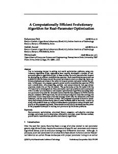
We should not expect these scalar quantities to change as a function of the number of terms, t, carried through the calculation in Equation 10. Therefore analysis of the ds and H as a function of t also enables the determination of an adequate number of terms to propagate through the retrieval. An example of using ds and H is shown in Figure 1 using the system setup described in Section III. In Figure 1 we show both ds and H as a function of the number of terms allowed to propagate through the retrieval, t. Even though only ≈90% of the variance is explained, ds and H do not vary with t≥3 terms indicating that at minimum, the retrieval should require t + 1 = 4 calls per channel to the RTA to calculate derivatives. Due to the use of 9 retrieval basis functions, the current implementation of the operational algorithm for IASI

8

Polar

6

Midlatitude

Information Content (bits) Degrees of Freedom Percent Variance Explained

90

Tropical

4

85

2

80

3

model sensitivities in temperature, moisture as well as trace gas species (CO, O3 , CH4 , CO2 , etc.). For the retrieval of CO we selected 33 channels in the 4.5µm region of the 1-0 vibration-rotation CO fundamental based on their signal-tonoise ratio (including geophysical uncertainties) and vertical extent of sensitivity.

95 Percent Variance Explained, [1]

Information Content/Degrees of Freedom, [1]


III. C OMPARISON OF AIRS S CIENCE T EAM R ETRIEVAL MAP R ETRIEVAL M ETHODOLOGY U SING IASI DATA

TO 0 2

4 6 Number of Terms, [1]

8

75 10

Fig. 1. CO retrieval ds and H as a function of t for clear tropical, midlatitude and polar atmospheres using IASI data.

In the following, we compare and contrast IASI retrievals for 10/19/2007 over the tropical range (latitudes between ± 30 degrees) using both the AST retrieval methodology and the MAP methodology described in previous sections. A. Averaging Kernels and Error Estimates

(13)

where σ(i) are standard deviations defined on coarse layers and interpolated onto the RTA grid scheme, p are the pressure layers of the RTA [3] and δP = 500hPa. The coarse layer σ’s and pressures are defined in Table I. Between the surface and 200hPa, σ values and pressures were determined by examination of the variance of NOAA/Earth Systems Research Laboratory/Global Monitoring Division (ESRL/GMD) aircraft CO data [11]. Above 200hPa, where both a priori information from in situ CO measurements and IASI’s measurement information becomes limited, we prescribe an ad-hoc decrease to the variances. Due to the fact that IR sounder sensitivity to CO above 200hPa is limited (see Section III-A), limitation of the variability in Sa above 200hPa is warranted. 2) Maintaining Near-Linearity in the Forward Model Derivatives: In the thermal IR, relative or logarithmic changes in layer column density are more linear than absolute changes in layer column density for trace gaseous constituents such as H2 O, O3 , CO and CH4 . This is due to the fact that the contribution of these gases to emission/absorption in the the radiative transfer equation depends on the exponential of the layer integrated column amount (i.e., the Beer-LambertBouguer Law) [12]. As eigenvectors of a real symmetric matrix, ui ∈ [−1, 1]. Assuming that we choose to perturb the forward model using multiplicative perturbations setting u = α, with x = (1.0 + α) · x, may create a problem with linearity as our perturbations will be in some cases close to 100%. In practice, we scale our original transformations by letting U = a0 · U, where a0 < 1.0. Factoring this scalar throughout our inversion equation requires scaling of all quantities including Σ = a−2 0 · Σ. Thus small perturbations to the forward model can be assured. B. Channel Selection and Radiative Transfer IASI CO retrievals utilize a prototype RTA based on the AIRS operational RTA [3], [9], which includes the ability to

Retrieval CO at 500hPa 300

AST Algorithm MAP Algorithm

250 CO, [ppbv]

Sa (i, j) = σ(i)σ(j) · exp(−|p(i) − p(j)|/δP )

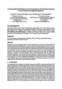
Figure 2 shows a comparison of the AST (purple) and MAP (green) retrieval algorithms at 500 hPa as a function of latitude (top panel) and shown as a function of pressure as a scattergram (bottom panel). Immediately apparent from the bottom panel, the most notable differences are for the upper and lower layers at 50 hPa and 900 hPa. These differences are due to the smoothing constraints on the retrievals.

200 150 100 50 -30

AST Algorithm CO, [ppbv]

requires ≈2× the number of calls to the RTA. This fact implies that the MAP retrieval will be at least twice as fast in the calculation of derivatives. The a priori covariance for the previous analysis was defined ad hoc as:

-20

-10

0 Latitude, [deg.]

10

20

30

300

900hPa 700hPa 500hPa 200hPa 50hPa

250 200 150 100 50 50

100

150 200 MAP Algorithm CO, [ppbv]

250

300

Fig. 2. Comparison of AST (purple) and MAP (green) retrieval algorithms at 500 hPa as a function of latitude (top panel) and shown as a function of pressure as a scattergram (bottom panel). Colored dotted lines in the bottom panel show uncertainty envelopes for theoretically calculated error estimates (see text). The individual pressures are plotted as various symbols and colors.

In the case of the AST approach, the primary smoothing constraint is the use of trapezoidal basis functions [12]. For the MAP retrieval, eigenvectors of Sa , Ut , serve as the primary smoothness constraint. As shown in Figure 2, at 50 hPa the AST retrieval basis functions correlate instrument sensitivity from layers below such that the variability introduced in the stratosphere is unphysical. For instance, in the most extreme cases (between -15 and -5 degrees latitude) the retrieval modifies the prior by almost 100%. Near the surface, the AST retrieval relaxes back to its a priori, due to the algorithm’s lack of an a priori smoothing constraint. The MAP retrievals behave in an opposite manner. Instrument sensitivity at 5 km is correlated with the prior constraint in Ut to enable the retrieval to move the bottom of the atmosphere. In the stratosphere,


Pressure (hPa) σ (%)

1100 66.7

800 40.0

600 40.0

400 33.3

200 20.0

100 10.0

4

50 6.67

10 3.33

1 0.66

0.01 0.66

TABLE I C OARSE P RESSURES AND P ERCENT VARIABILITIES , σ, U SED T O D EFINE T HE ad hoc a priori C OVARIANCE , Sa .

namely the use of trapezoidal basis functions, impart large vertical scale correlations between the middle troposphere and higher altitudes. The fact that our uncertainty curves were calculated for a MAP algorithm, which does does not include the ability to characterize the correlation of the AST algorithm, explains that discrepancy between the uncertainty curves and the difference between the AST and MAP algorithms above 200hPa. lat: 16.61S, lon: 38.55W

dof(AST): 1.22, dfs(MAP): 1.19

25

25

AST

AST Algorithm

MAP

20

20

A Priori

Pressure Altitude, [km]

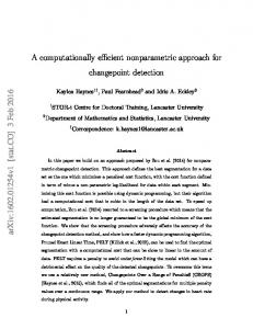
the MAP retrievals relax back to the a priori due to the combination of low magnitude prescribed variability in Ut and lack of instrument sensitivity. Propagation of error techniques [8] provide a better gauge to the similarities and differences between the two retrieval algorithms. For instance, in the bottom panel of Figure 2 we show theoretically calculated total uncertainties (sum of spectrally interfering species as well as instrument N E∆T and averaging kernel smoothing) for a nominal tropical atmosphere. For background species, we used 1K errors for surface temperature, and formed error covariances using Equation 13 and coarse layer σ’s and pressures for temperature and moisture as defined in Table II with correlation parameters: δP = 700hPa for temperature and δP = 300hPa for moisture. Coarse layer σ’s in Table II were estimated using our current knowledge of temperature and moisture uncertainty from IASI as matched to an operational radiosonde database [13], [14]. With the exception of the extremely high CO abundances (biomass burning regions), Figure 2 shows that both retrieval methodologies give similar results between 300-700hPa altitude. The differences for the large values could be due to either underconstrained AST retrievals or overconstrained MAP retrievals. Total column retrievals (not shown) show good agreement, which indicate the opposite magnitude differences as a function of altitude between each of the retrieval methodologies counteract each other resulting in better agreement in the integral CO abundance. Figure 3 shows example retrieved CO profiles for each algorithm over Brazil as well as corresponding averaging kernels, A. A, describe the sensitivity of each retrieval algorithm to changes in “true” CO and further illustrate the differences in the retrieval algorithm constraints. The degrees of freedom, dof for the AST algorithm [12] and the degrees of freedom for signal, df s, for the MAP retrieval algorithm [8] are listed at the top of the right panel. Differences in the vertical constraints used in the two algorithms are further evident from the left panel in Figure 3 where the enhanced CO retrieved from the AST algorithm (blue line between 8 and 5 km) is partially offset by the enhancement in the MAP retrieved CO (red line below 2 km). For pressures below 200hPa, the uncertainty curves in Figure 2 act as envelopes to the differences between the two algorithms indicating that the differences are within expected retrieval uncertainty. At 200hPa and 50hPa, the differences between the two retrieval algorithms are outside of the uncertainty curves for 6% and 55% of cases. This behavior can be best understood through inspection of the averaging kernels shown in Figure 3. Above 200hPa, middle tropospheric averaging kernels for the AST algorithm decay toward zero slower than middle tropospheric averaging kernels for the MAP algorithm and indicate that the smoothness constraints in the AST algorithm,

MAP Algorithm

15

15

10

10

5

5

0

1 hPa 9 hPa 32 hPa 71 hPa 142 hPa 235 hPa 374 hPa 535 hPa 753 hPa 1013 hPa

0 50

100 150 CO, [ppbv]

200

250

0.00 0.02 0.04 0.06 Averaging Kernel, [1]

Fig. 3. The left panel shows a comparison of AST (blue) and MAP (red) CO retrievals over Brazil on 10/19/2007 using IASI cloud-cleared measurements. The right panel shows AST (dashed) and MAP (solid) averaging kernels, which describe the vertical sensitivity of each algorithm, colored as a function of pressure for the corresponding case. Degrees of freedom, dof , for the AST and degrees of freedom for signal, df s, for the MAP retrievals are listed at the top of the right panel.

The general agreement between the two unrelated retrieval methodologies in mixing ratios between 300-700 hPa and total column abundances, strengthens the indication from the dof and df s in Figure 3 that the sensitivity of IASI measurements to CO variability is limited to around 1 degree of freedom in the vertical weighted toward 300-700hPa. IV. C ONCLUSIONS AND O UTLOOK In this letter we have described a novel and fast approach to the implementation of the MAP method for the derivation of CO from IASI cloud-cleared measurements. Although the algorithm demonstration and comparison contained in this letter focused on the use of IASI data to derive CO, the algorithm is flexible enough for use with any hyperspectral sounder dataset (e.g. AIRS, IASI, or CrIS) and target parameter where a priori information is available. For instance, we have successfully applied the algorithm principles to retrievals of temperature, ozone and CO2 and are currently preparing manuscripts for consideration for publication in various journals.


Pressure (hPa) σ (K)

1100 1.25

800 1.0

Temperature 500 300 1.0 1.25

200 1.5

100 1.5

5

10 1.75

1100 20

Water 600 400 30 30

200 60

TABLE II C OARSE P RESSURES AND P ERCENT VARIABILITIES , σ, U SED T O D EFINE T HE ad hoc C OVARIANCE M ATRICES FOR T EMPERATURE AND M OISTURE , Sb .

Using a theoretical analysis of IASI sensitivities we have shown that for CO the expectation of performance is approximately 10-15% in the middle troposphere with slightly larger errors near the surface. Comparing the MAP retrieval with the AST retrieval on real data, we find that both retrieval methodologies yield answers within this precision estimate in the middle troposphere; however, although well constrained by theoretical error estimates (see Figure 2), the differences between the algorithms are larger approaching the surface and in the upper troposphere. These facts indicate that both the IASI algorithms are currently sensitive to approximately 1 piece of information highly weighted toward the middle troposphere. Nevertheless, it is our expectation that higher sensitivities will tend toward the surface in regions of strong thermal gradients between tropospheric and surface temperatures and in strictly clear scenes. ACKNOWLEDGMENT The authors wish to thank Tom King and acknowledge the efforts of the NOAA/NESDIS/STAR/IOSSPDT team that enabled this analysis of the IASI data the two anonymous reviewers for their helpful comments. R EFERENCES [1] F. Cayla, “IASI infrared interferometer for operations and research,” NATO ASI Series-I (eds. Chédin, Chahine, Scott), Tech. Rep., 1993. [2] H. H. Aumann, M. Chahine, C. Gautier, M. Goldberg, E. Kalnay, L. McMillin, H. Revercomb, P. Rosenkranz, W. Smith, D. Staelin, L. Strow, and J. Susskind, “AIRS/AMSU/HSB on the Aqua mission: Design, science objectives, data products and processing systems,” IEEE Trans. Geosci. Remote Sensing, vol. 41, no. 2, 2003. [3] L. Strow, H. Motteler, S. Hannon, and S. De Souza-Machado, “An overview of the AIRS radiative transfer model,” IEEE Trans. Geosci. Remote Sensing, vol. 41, no. 2, 2003. [4] M. Goldberg, L. Qu, Y. McMillin, W. Wolf, L. Zhou, and M. Divakarla, “Airs near-real-time products and algorithms in support of operational weather prediction.” IEEE Trans. Geosci. Remote Sensing, vol. 41, pp. 379–389, 2003. [5] L. Zhou, M. Goldberg, C. D. Barnet, Z. Cheng, F. Sun, W. Wolf, T. King, X. Liu, H. Sun, and M. Divakarla, “Regression of surface spectral emissivity from hyperspectral instruments,” IEEE Trans. Geosci. Remote Sensing, vol. 46, no. 2, 2008. [6] J. Susskind, C. D. Barnet, and J. Blaisdell, “Retrieval of atmospheric and surface parameters from AIRS/AMSU/HSB data in the presence of clouds,” IEEE Trans. Geosci. Remote Sensing, vol. 41, no. 2, 2003. [7] C. D. Rodgers, “Characterization and error analysis of profiles retrieved from remote sounding measurements,” JGR, vol. 95, no. D5, pp. 5587– 5595, 1990. [8] ——, Inverse methods for atmospheric sounding: Theory and practice. World Scientific Publishing, 2000. [9] L. L. Strow, S. E. Hannon, S. De-Souza Machado, H. E. Motteler, and D. C. Tobin, “Validation of the atmospheric infrared sounder radiative transfer algorithm,” J. Geophys. Res., vol. 111, no. D09S06, 2006. [10] S.-A. Boukabara, F. Weng, and Q. Liu, “Passive microwave remote sensing of extreme weather events using noaa-18 amsua and mhs,” IEEE Trans. Geosci. Remote Sensing, vol. 45, no. 7, pp. 2228–2246, 2007. [11] C. Sweeney, 2006, private communication.

[12] E. S. Maddy and C. D. Barnet, “Vertical Resolution Estimates in Version 5 of AIRS Operational Retrievals,” IEEE Transactions on Geoscience and Remote Sensing, vol. 46, pp. 2375–2384, Aug. 2008. [13] M. G. Divakarla, C. D. Barnet, M. D. Goldberg, L. M. McMillin, E. Maddy, W. Wolf, L. Zhou, and X. Liu, “Validation of Atmospheric Infrared Sounder temperature and water vapor retrievals with matched radiosonde measurements and forecasts,” Journal of Geophysical Research (Atmospheres), vol. 111, no. D10, pp. 9–+, apr 2006. [14] M. Divakarla, 2009, personal communication.

Eric Maddy Eric Maddy received degrees in physics and mathematics (2001) from Frostburg State University, Frostburg, MD. He received his MS and Ph.D degrees in Atmospheric Physics from the University of Maryland, Baltimore County (UMBC) in 2003 and 2007 respectively. He has been with QSS Group, Inc./Perot Systems Government Services (PSGS), Inc., Lanham, MD since 2004, focusing on the development and analysis of algorithms for deriving temperature, moisture and carbon trace gases from operational hyperspectral sounders.

Chris Barnet Christopher Barnet received degrees in electronics technology (1976) and solid state physics (1978) from Northern Illinois University, DeKalb. In 1990 he received his Ph.D. degree from New Mexico State University, Las Cruces in remote sensing of planetary atmospheres using visible and infrared instruments aboard the Voyager spacecraft. Since 1995 he has worked on advanced algorithms for terrestrial infrared and microwave remote sensing and has actively supported NASA’s Advanced Infrared Sounder (AIRS) science team and the NPOESS Sounder Operational Algorithm Team (SOAT). In June 2003 he joined the Office of Research and Applications (ORA) of NOAA/NESDIS where he is exploiting operational sounder missions to provide the first global understanding of carbon monoxide, carbon dioxide, and methane in the free troposphere. These measurements, will contribute to the understanding of the terrestrial carbon cycle and climate change.

Antonia Gambacorta Antonia Gambacorta received her degree in Physics (2001) from the Universitá degli Studi di Bari, Italy. She received her MS and Ph.D. in Atmospheric Physics from the University of Maryland, Baltimore County in 2004 and 2008 respectively. In October 2006, she joined the QSS Group, Inc./Perot Systems Government Services (PSGS), Inc., working at NOAA/NESDIS in Camp Springs, MD. Her research focuses on inversion algorithms and product analysis from hyperspectral sounders and climate applications in the field of the hydrological cycle.