We took the Common LISP constraints library SCREAMER and extended its symbolic capabilities to suit our purposes. Additionally, we formulated an example ...
A Constraint-Based Approach to the Description of Competence S. White and D. Sleeman Department of Computing Science, King’s College, University of Aberdeen, Aberdeen, AB24 3UE Scotland, UK. Tel.: +44 (0)1224 272296; Fax.: +44 (0)1224 273422 Email: @csd.abdn.ac.uk
Abstract. A competency description of a software component seeks to describe what the artefact can and cannot do. We focus on a particular kind of competence, called fitness-for-purpose, which specifies whether running a software component with a supplied set of inputs can satisfy a given goal. In particular, we wish to assess whether a chosen problem solver, together with one or more knowledge bases, can satisfy a given (problem solving) goal. In general, this is an intractable problem. We have therefore introduced an effective, practical, approximation to fitness-for-purpose based on the plausibility of the goal. We believe that constraint (logic) programming provides a natural approach to the implementation of such approximations. We took the Common LISP constraints library SCREAMER and extended its symbolic capabilities to suit our purposes. Additionally, we formulated an example of fitness-for-purpose modelling using this enhanced library.
1 Introduction A competency description of a software component seeks to describe what the artefact can do, and what it cannot do. In addition, it may choose to describe the methods that are applied by the software artefact to achieve its results, although our work focuses on the questions of what rather than how. Competency descriptions can enable human- or machine agents to assess the suitability of application of the described component for some particular task. This assessment of suitability, which we also refer to as fitness-for-purpose analysis, is becoming increasingly important for two main reasons. Firstly, as the range and sophistication of software increases, it becomes difficult for a human user to make an informed choice of the best software solution for any particular task. The same point applies equally to domain independent reasoning components, such as the problem solving methods (PSMs). We believe that novice users, in particular, could benefit greatly from advice generated as a result of a fitness-for-purpose analysis. Secondly, we observe a demand for software brokers, which, given some software requirements, return either the soft-
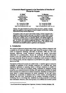
ware itself, or a pointer. In the knowledge acquisition community, the IBROW3 project [3] intends to build such a broker for the distribution of problem solving components. In this paper, we present a general approach to fitness-for-purpose analysis which was developed to assist in the generation of advice for novice users of knowledge acquisition tools (KA tools) and problem-solvers in the MUSKRAT system [10], [24], [27]. MUSKRAT is a MUltiStrategy Knowledge Refinement and Acquisition Toolbox which makes it easier for novice users to apply and combine the incorporated software tools to solve some specific task. When generating advice on the application of a chosen problem-solver, MUSKRAT should be able to differentiate between the following three cases for the knowledge bases available to the problem-solver. Case 1: The problem-solver can be applied with the knowledge bases already available, i.e., no acquisition or modification of knowledge is necessary. Case 2: The problem-solver needs knowledge base(s), not currently available; therefore these knowledge base(s) must be first acquired. Case 3: The problem-solver needs knowledge base(s), not currently available, but the requirements can be met by modifying existing knowledge base(s). The phrase ‘fitness-for-purpose’ and the computational approximation to it, as described in this paper, arose out of the need for a test for case 1. We expect subsequent research to investigate issues relating to cases 2 and 3. Issues related to the description of competence are also being investigated by others in the field, notably Benjamins et al. in the context of the IBROW3 project [3], [4], Fensel et al., as part of an ongoing investigation into the role of assumptions [6], [7], and Wielinga et al., as a methodological approach to the operationalisation of knowledgelevel specifications [30]. We consider Fensel’s approach to be the nearest to our work, because it investigates the context dependency of an existing problem solver/PSM through the discovery of assumptions. We are also investigating the context dependency of problem solvers, but through the question of task suitability with the available knowledge. Thus, whilst Fensel investigates a problem solving method in isolation of its inputs in order to derive suitability conditions, we take a problem solver together with its inputs and test their combined suitability for solving a specific task. Both lines of inquiry are intractable, and therefore demand some compromise(s) in any implementation. Fensel’s compromise concerns the level of automation of his proof mechanism, which is an interactive verifier, rather than a fully automated proof mechanism. Since we would like to generate advice at run-time for the potential user of a problem solver, we compromise instead with the deductive power of our proof mechanism. We believe, however, that what our constraint satisfaction mechanism may lack in expressive power, it gains in its abilities to combine the results of multiple problem solvers (through propagation mechanisms), and run as a batch process. Figure 1 compares Fensel et al.’s process of assumption hunting with our approach to matching a problem solver to a toolkit user’s goal.
PSM
PSM
Abstract
Formalise Goal
Goal
KBs
Prove Competence
(Dis)Prove Goal
(using Karlsruhe Interactive Verifier)
(using Constraint Satisfaction)
Properties
Properties
(Assumptions)
(Compatibility of Goal/PSM/KBs)
(i)
(ii)
Figure 1. Comparison of the Fensel approach (i), and our approach (ii), to the discovery of problem solving properties
In the following section, we define more exactly what we mean by fitness-for-purpose, and explain the computational difficulties which arise in its analysis. In section 3, we describe how we approach these difficulties by considering an approximation of fitness-for-purpose, rather than the actual fitness-for-purpose. In section 4, we explain how we are implementing these ideas using constraint logic programming in Common LISP. Finally, in section 5 we summarise the ideas, relate them to other work in the field, and indicate some possible directions for future work.
2 Fitness-for-Purpose In the previous section, we defined a competency description of a software component as a description of what the artefact can do, and what it cannot do. Since a fitness-forpurpose analysis considers the suitability of some component for a particular task instance, it concerns not only the ‘absolute’ competence of that component for contributing to the solution, but also any other inputs which the component, or the task, might have. So, for example, a kettle undoubtedly has a competence for boiling water, but it is nevertheless not fit for the purpose of making a cup of tea unless water, tea and (optionally) milk and sugar are also available. Fitness-for-purpose therefore represents a specific interpretation of ‘competence’, because it expresses the contribution to the solution of the problem instance with regard to the current state of the containing system. In the tea-making example, the ‘current state’ concerned the availability of ingredients in the kitchen; in the context of knowledge acquisition and problem solving, the current state refers to the availability and nature of the system’s knowledge.
When the advisory subsystem of MUSKRAT addresses the problem of fitness-for-purpose, it is in effect posing the question “Is it possible to solve the given task instance with the available problem-solver1, knowledge bases, and KA tools?”. Clearly, this is a very difficult question to answer without actually running the problem-solver, regardless of whether the answer is generated by a human or a machine. Indeed, the theory of computation has shown that it not possible, in general, to determine whether a program (in this case, a problem-solver) terminates. This is the Halting Problem [25]. Therefore the only way to affirm the suitability of a problem-solver for solving a particular task is to run it and test the outcome against the goal. For the purposes of generating advice in a multistrategy toolbox, however, we cannot afford this luxury, particularly since running the problem-solver could itself be computationally intensive. We prefer instead to pose the weaker question “Is it plausible that the given task instance could be solved with the available problem-solver, knowledge bases, and KA tools?”. We believe that it is possible to demonstrate computationally that some configurations of a task, problem-solver, existing knowledge bases and KA tools cannot, even in principle, generate an acceptable solution to the task. Such situations form a set of recognisably implausible configurations with respect to the problem at hand. Furthermore, the computational cost associated with recognising this implausibility is, in many cases, far less than that associated with running the problem-solver. For example, consider a question from simple arithmetic: is it true that 22 × 31 + 11 × 17 + 13 × 19 = 1097 ? Rather than evaluate the left hand side of the equation straight away, let us first inspect the problem to see if it is reasonable. We know that when an even number is multiplied by an odd number, the result is always even; and that an odd number multiplied by an odd number is always odd. Therefore the left hand side of the equation could be rewritten as + + . Likewise, an even number added to an odd number is always odd, and the sum of two odd numbers is always even. Then evaluating left to right, we have + , which is . Since 1097 is not even, it cannot be the result of the evaluation. We have thus answered the question without having to do the ‘hard’ work of evaluating the actual value of the left hand side. As another example, consider the truth of the statement ‘If Pigs can fly, then I’m the Queen of Sheba’, which we write as P ⇒ Q. Given our background knowledge that the premise P is false, we can use the truth table for logical implication2 to derive that the whole statement is true, since any implication with a false premise is true. Notice that we derived our result without having to know the truth of the consequent Q. In a similar way, it is possible to investigate the outputs of programs (in particular, problem 1. For simplicity, we currently assume the application of a single, chosen problem-solver. 2.
P T T F F
Q T F T F
P⇒Q T F T T
solvers) without needing complete information about their inputs. This issue becomes important if running a problem solver has a high cost associated with it, such as the time it takes to perform an intensive search3. In such cases, a preliminary investigation of the plausibility of the task at hand could save much time if the intended problem solver configuration can be shown to be unsuitable for the task. We consider such an investigation to be a kind of ‘plausibility test’ which should be carried out before running the actual problem solver. The idea was suggested as part of a general problem solving framework by Polya [19]. In his book ‘How to Solve It’, he proposed some general heuristics for tackling problems of a mathematical nature, including an initial inspection of the problem to understand the condition that must be satisfied by its solution. For example, is the condition sufficient to determine the problem’s “unknown”? And is there redundancy or contradiction in the condition? Polya summarised by asking the following: ‘Is our problem “reasonable”? This question is useful at an early stage of our work if we can answer it easily. If the answer is difficult to obtain, the trouble we have in obtaining it may outweigh the gain in interest.’ (Polya, 1957).4 It is interesting to note that the arithmetic example given above first abstracts the problem instance to a different ‘space’ (i.e., from real numbers to that of odd and even numbers), to which a simpler algebra can be applied. We note that much of the problem instance detail has been ignored to keep the plausibility test simple. On the other hand, enough detail has been retained for the test to reflect the current problem instance and for it to be useful. In this sense, the plausibility test has approximated the task. In the next section, we define a more precise notion of plausibility approximation, and explain how it can be applied to problem-solvers.
3 The Plausibility Approximation to Fitness-for-Purpose We classify proposed solutions to a problem as either plausible values, candidate values, or actual values. Informally, a plausible value is any solution which cannot be ruled out by applying such reasoning as that in the arithmetic or logical examples above. A candidate value can be a solution to the problem in some cases. An actual value is the solution in a given case. It is worth noting that all candidate solutions are also plausible, and any actual solution is always a candidate solution (see Figure 2).
3. Many AI programs perform searches of problem spaces which grow exponentially with the size of the problem. 4. One way to determine whether the plausibility test is useful is to compare the computational complexities of the problem solver and the plausibility test. If the order of complexity of the plausibility test is lower than that of the problem solver, we might assume it is reasonable to apply the plausibility test first. Unfortunately, this model takes no account of the utility of the information gained from the plausibility test.
An Actual Solution
Universal Set
Set of Plausible Solutions
Set of Candidate Solutions
Figure 2. Venn Diagram showing the relationships between plausible, candidate, and actual solutions
As an example of this classification, consider the formula for the area of a circle, πr2. Suppose that we know r, the radius, to be larger than 1, but no greater than 10, i.e., r ∈[1, 10] and r2 ∈[1, 100]. Now we should like to define ranges of plausibility and candidacy for the value of the circle’s area. The range of candidate values is [π, 100π], but since π is rather a difficult number to deal with, the calculation of plausibility might approximate it to 3 for estimating the lower bound of the range, and 3.5 for estimating the upper bound of the range. The lower bound of the range is therefore lower_bound(r2) × 3 = 3; and the upper bound is upper_bound(r2) × 3.5 = 350. This gives the range of plausibility as [3, 350]. Note that we were careful to underestimate the lower bound of the plausibility range, and overestimate the upper bound, so that the range of candidate values lies completely within the range of plausible values (c.f. the theory of errors used in the empirical sciences). When evaluating the expression, an actual value might be 78.54. The set of plausible solutions is an approximation to the set of candidate solutions, but we define it such that the set of candidate solutions is always contained within the set of plausible solutions. This guarantees that an implausible solution is not a candidate solution, so we can approximate the test for candidacy with a test for plausibility. Note that a plausible solution may not necessarily be a candidate – plausible, but non-candidate, solutions are the ‘small fish’ that slip through the net! Note also that for any gain in computational effort, testing an element for membership of the set of plausible solutions must be in some sense less expensive than testing it for membership of the set of candidate solutions. We are applying these ideas to problem solving scenarios in which a number of knowledge bases (KB1, KB2, ..., KBn) are assigned input roles (R1, R2, ..., Rn) to a problem-
solver, and a desired goal G is stated. We call this a problem-solver configuration (left hand side of Figure 3). Note that at this stage we have made no assumptions about the representation of the knowledge; when we say ‘knowledge base’ we do not imply a set of rules. Neither do we make any assumptions about the specificity of the knowledge bases with respect to the given problem instance. (That is, a knowledge base might remain constant over all problem instances, it might change occasionally, or it might change with every instance.) In essence, any input to the problem-solver has been labelled as a knowledge base. We use the knowledge obtained from these inputs and a plausibility ‘description’ of the behaviour of the problem-solver to generate an output space of plausible values. Note that under this scheme, a problem-solver ‘description’ is itself a program which implicitly describes another program by generating its plausible output. The description therefore represents a kind of model of the problem solving task; it is a metaproblem-solver (right hand side of Figure 3). The aim of the model is to determine whether the goal G is consistent with the plausible space generated by the metaproblem-solver, because if G is not consistent with this space, then it will also not be satisfied by the output of the problem-solver itself. In such cases, we need not run the problem-solver to test its outcome. But how can this functionality be implemented? In a naive generate-and-test approach, we might answer the plausibility question by testing every point in the plausibility space against the goal G. Unfortunately, this is both computationally inefficient [13], and enables only the modelling of spaces of finite size. For a more flexible and computationally more efficient version, we prefer a constraint-based approach5. The idea is that a plausibility space is expressed as a set of constrained entities. This set could be of infinite, or indefinite, size, such as the set of even counting numbers, or the set of all persons whose surname begins with ‘W’. To test the plausibility of a given goal, its features are applied as further constraints to the plausibility space generated by a metaproblem-solver. If the resulting space is empty, then the goal was not plausible; if the resulting space is non-empty (or cannot easily be demonstrated to be empty), then the goal remains plausible. Furthermore, unlike the meta-level reasoning required for the halting problem, the question of plausibility, if defined appropriately, can be guaranteed to terminate within a finite number of program steps, because the meta-level need only be an approximation to the problem solving level6.
5. Consider the whimsical analogy of a man wishing to buy a pair of shoes: he does not walk into a bookshop, pick up every book, and inspect it for its shoe-like qualities (the generateand-test approach). Instead, he recognises from the outset that bookshops sell books (i.e. the plausibility space is a set of books), and that this is not consistent with his goal of buying shoes. 6. Consider the case of the halting problem, in which we should like to determine whether a program runs forever or halts. At the meta-level, we may choose to run the program for some given length of time to see what happens. If the program halts within the allotted time, then we know that it halts. Otherwise it remains plausible that it runs forever.
Metaproblem-solver
Problem-solver
KB1
KB1
KBn
R1
R1
Rn
satisfies?
Rn
Meta Problem-solver
Problem-solver
Output O
KBn
Goal G
consistent with?
Plausibility Space P
Key R
Knowledge Base (KB)
Program produces output
Program Component Space of Plausible Knowledge
KB used as input in Role R
Rel
Relationship between KBs
Figure 3. Problem-solver and Metaproblem-solver Configurations
Note that the plausibility refers to the combination of knowledge bases, their problemsolving roles and the specific goal. In principle, a reassignment of knowledge bases to different problem-solving roles could transform an implausible configuration into one which is plausible. To avoid such anomalies, we also assign preconditions to each problem solving role, and check that these are fulfilled by a knowledge base before conducting a plausibility test. More general scenarios are also possible, since plausibility spaces can also be used as inputs to further metaproblem-solvers. Such an input space could describe the plausible output of another problem-solver, or even a knowledge acquisition tool. By cascading descriptions in this way, plausibility spaces are combined. When plausibility spaces are used as inputs to metaproblem-solvers, the plausible output space produced is necessarily more general than when specific knowledge bases are used as inputs.
Nevertheless, the output space may still contain enough knowledge to answer some interesting questions.
4 Implementation Approach We mentioned earlier that we prefer a constraint-based approach to answering the question “Is the goal G contained in the plausibility space P ?”. In fact, it is crucial to the implementation that constraints derived from the goal can be used to reduce the size of the plausibility space without enumerating it. This technique makes the plausibility test less expensive than running the problem-solver because the whole search space does not have to be explored to determine whether a goal is implausible. It also leads one naturally to consider an implementation using constraint (logic) programming. Indeed, we can rephrase the plausibility question in the terminology of constraint programming: “Is the goal G consistent with the domain of the constraint variable P ?”. Since the tools we wished to model and the rest of the MUSKRAT framework were already implemented in Common LISP, we sought to implement the plausibility approximation to fitness-for-purpose using SCREAMER, a constraint logic programming library for Common LISP [22], [23]. 4.1 A Brief Introduction to SCREAMER and SCREAMER+ SCREAMER introduced two paradigms into Common LISP: firstly, it introduced a nondeterminism similar to the backtracking capabilities of PROLOG. Secondly, and more importantly for our purposes, it used these backtracking capabilities as the foundation for a declarative constraints package. The SCREAMER constraints package provides LISP functions which enable a programmer to create constraint variables, (often referred to simply as variables), assert constraints on those variables, and search for assignments of values to variables according to the asserted constraints. Although SCREAMER7 forms a very good basis for solving numeric constraint problems in Common LISP, we found it less good for tackling problems based on constraints of a more symbolic nature. We therefore extended the S CREAMER library in three major directions: firstly, to improve the expressiveness of the library with respect to constraints on lists; secondly, to introduce higher order8 constraint functions such as constraint-oriented versions of the LISP functions every, some, and mapcar; and thirdly, to enable constraints to be imposed on CLOS9 objects and their slots. We called the extended library SCREAMER+. A detailed discussion of SCREAMER+ is
7. Version 3.20; available at the time of writing from http://www.cis.upenn.edu/ ~screamer-tools/home.html
8. A ‘higher order function’ is a function which accepts another function as an argument. 9. CLOS is the Common LISP Object System, a specification of functions to enable object-oriented programming in LISP which was adopted by the ANSI committee X3J13 in 1988 as part of the Common LISP standard.
outside the scope of this paper; the interested reader is referred to our recent technical report [28]. In the next section, we provide an example of the usage of the SCREAMER+ library to model the fitness-for-purpose of two problem-solvers applied to the domain of meal preparation. 4.2 A Problem Solving Scenario Dish Ontology
Available Resources Dish Preferences
Component Instances
Dish Recipes
Set of Constraints Designer
Single Dish
satisfies?
Required Dish
Figure 4. Problem Solving in the Domain of Meal Preparation
Suppose we are applying a problem-solver which constructs solutions consistent with some given domain and temporal constraints (a design task)10. We have chosen to apply the problem-solver to the domain of meal preparation because the domain is rich and challenging, but also easily understood. Furthermore, the problem-solving task is analogous to flexible design and manufacturing, also called just-in-time manufacturing. In the domain of meal preparation, the designer is used to compose (or ‘construct’) a dish which is consistent with culinary, temporal, and resource constraints, also taking a set of dish preferences into consideration (see Figure 4). Now suppose that we would like to use plausibility modelling on this problem-solver by constructing its corresponding metaproblem-solver. A meta-designer is easy to construct if we neglect the constraints, dish preferences, and the available resources. The meta-designer produces a space of plausible dishes, together with their plausible preparation times. These times are represented as upper and lower bounds on the preparation of whole dishes, and are derived from knowledge of the preparation times of dish
10.The task is also soluble by two separate problem solvers: the domain constraints are solved by the first, and the temporal constraints satisfied by the second [29]. A detailed discussion of the cascading of problem solvers is outside the scope of this paper.
Component Instances
Dish Ontology
Dish Recipes
MetaDesigner
Required Dish
consistent with?
Plausible Dish Space
Figure 5. Plausibility Reasoning in the Domain of Meal Preparation
components. The upper bound of the dish preparation time is set as the sum of the durations of the composite tasks; the lower bound is the duration of the lengthiest task. Constraints from the goal can then be applied to the space of plausible scheduled dishes to see if inconsistencies can be detected (see Figure 5). Note that although we advocate the use of the constraint satisfaction paradigm for the implementation of the meta-level, this choice is independent of the implementation method used by the problem solver itself. The independence arises because the meta-layer treats the problem solver as a black box, describing only its input/output relationship and not how it works internally. 4.3 An Implementation of Plausibility We have implemented a prototype of plausibility reasoning by using the knowledge provided in Table 1: a list of dish components, together with their component type, a measure of their dietary value, their cost and preparation time. In addition, the designer must be told what it should construct from this knowledge. This information is provided by a dish ontology which states that a dish consists of a main component, together with a carbohydrate component and two other vegetables. Likewise, the cost of a dish is defined to be the sum of the costs of its component parts, and the number of diet points associated with a dish is the sum of the diet points of its components. The meta-designer generates upper and lower bounds for the preparation time of a dish, as described in the previous section. The SCREAMER+ implementation makes use of the CLOS facilities offered by defining the space of plausible dishes as a single object in which each slot (such as the main component of the dish, the preparation time, dietary points value, and cost) is constrained to be plausible. In practice, this means that constraints are expressed across
Ingredient Name
Ingredient Type
Diet pointsa
Cost (£)
Preparation Time (mins)
Lamb Chop
Main (meat)
7
4
20
Gammon Steak
Main (meat)
10
4
15
Fillet of Plaice
Main (fish)
8
4
15
Sausages
Main (meat)
8
2
10
Chicken Kiev
Main (meat)
8
3
30
Quorn Taco
Main (vegetarian)
6
3
10
Jacket Potato
Carbohydrate
5
1
60
French Fries
Carbohydrate
6
1
15
Rice
Carbohydrate
6
1
15
Pasta
Carbohydrate
2
1
10
Runner Beans
Vegetable
1
1
10
Carrots
Vegetable
1
1
15
Cauliflower
Vegetable
1
1
10
Peas
Vegetable
2
1
3
Sweetcorn
Vegetable
2
1
5
a. Points schemes like these are commonly used by slimmers as a simplification of calorific value. When using such schemes, slimmers allow themselves to consume no more than, say, 40 points worth of food in a single day (the actual limit usually depends on the slimmer’s sex, height, and weight).
Table 1. Meal Preparation Knowledge Used in Plausibility Space Generation the slots within a single object. If the domain of one of the slot’s constraint variables changes, then this causes propagation to the other related slots. For example, let us inspect some plausible dish preparation times and costs: ;;; Create an instance of the object ;;; An after method asserts the appropriate constraints across ;;; the object’s slots at object creation time. USER: (setq my-dish (make-instance 'plausible-dish)) # ;;; Retrieve the value of the duration slot USER: (slot-value my-dish 'duration) [774 integer 10:120]
;;; Retrieve the value of the cost slot USER: (slot-value my-dish 'cost) [769 integer 5:7 enumerated-domain:(5 6 7)]
This tells us that a plausible dish takes between ten minutes and two hours to prepare, and costs £5, £6, or £7. Now let us restrict our search to a fish dish, and again inspect the plausible values: USER: (assert! (typepv (slot-valuev my-dish 'main) 'fish)) NIL USER: (slot-value my-dish 'duration) [774 integer 15:105] USER: (slot-value my-dish 'cost) 7
The plausible range size for the preparation time of the dish has decreased, and the cost of the dish has become bound without having to make any choices of vegetables. If the goal were to have such a fish dish ready in less than quarter of an hour, it would fail without having to know the details of the dish preferences or kitchen resources used by the actual problem-solver, and without needing to run the problem-solver: USER: (assert! (