numerous variants for the detection of lines, circles, ellipses and general polygonal .... Straight field lines of the playing field are either parallel or perpendicular.
A constructive feature detection approach for robotic vision Felix von Hundelshausen, Michael Schreiber, and Ra´ ul Rojas Free University of Berlin, Institute of Computer Science Takustr. 9, 14195 Berlin, Germany {hundelsh|schreibe|rojas}@inf.fu-berlin.de
Abstract. We describe a new method for detecting features on a marked RoboCup field. We implemented the framework for robots with omnidirectional vision, but the method can be easily adapted to other systems. The focus is on the recognition of the center circle and four different corners occurring in the penalty area. Our constructive approach differs from previous methods, in that we aim to detect a whole palette of different features, hierarchically ordered and possibly containing each other. Highlevel features, such as the center circle or the corners, are constructed from low-level features such as arcs and lines. The feature detection process starts with low-level features and iteratively constructs higher features. In RoboCup the method is valuable for robot self-localization; in other fields of application the method is useful for object recognition using shape information.
1
Introduction
Robot self-localization is an important problem in the RoboCup domain. Many systems rely on Monte Carlo Localization [19] identifying landmarks such as the colored goals or posts. There have been attempts to detect field line features and to use them for robot self-localization. In [18] straight lines are detected, however no other features, in particular no curved features are extracted. In [9] straight lines and circles are recognized using the Hough transform [10], but no other features like the corner circle sectors or the rectangle of the penalty area are detected. Although the Hough transform is robust and conceptually elegant, it is inefficient, since for each type of feature a separate parameter space has to be maintained. The search for local maxima in parameter space can be optimized by combining the method with Monte Carlo Localization, however it is still computationally expensive [9]. In this paper, we aim at efficient and robust feature recognition which allows the unique localization of the robot, up to the symmetry of the playing field. We refer to such features as high-level features in the following. We concentrate on five different high-level features: The center circle and four different corners which occur at the penalty area, as shown in Fig. 1. This paper contains two contributions. First, we propose methods which allow the robust and efficient detection of the features mentioned above. Second, and
right outer corner right inner corner
center circle
left inner corner left outer corner
Fig. 1. The center circle and four different corners are recognized by the system. Although the shapes of the different corners are identical, the system is able to identify the position of a detected corner within the penalty area. Within one side of the playing field, each of the corners represents a unique feature.
more important, we propose a framework which can be extended to recognize other feature types without doing all the work from scratch. Feature detection has been addressed in numerous papers: The simplest approach for feature detection is to directly derive parameters of the feature from the data. For instance, for three points (not all collinear) one can easily derive the parameters of the circle containing the points. However, one has to be sure that the points belong to a circle. If one point is wrong, a false circle will be constructed. The next class of methods is based on least-squares fitting. Instead of deriving the parameters with the minimum number of required points, more points are used and the total error is minimized. There exist fitting methods for lines (i.e see appendix of [13]), circles[17] and ellipses[8], or more generally for conic sections[7]. However it has to be know a priori which points belong to the feature. Outliers affect the result seriously. Therefore, attempts to develop robust detection methods have been made. The probably most robust are Hough transform[10] based methods. There exist numerous variants for the detection of lines, circles, ellipses and general polygonal shapes. Each input item (i.e a point) votes for all possible parameters of the desired feature and the votes are accumulated on a grid. The parameters with the most votes determine the feature. The counterpart of Hough transform methods, are techniques that probe parameter space. Instead of beginning with the input data and deriving the parameters in a bottom-up fashion, parameter space is searched top-down way[16, 3].
Other approaches, rely on the initial presence or generation of hypothesis. RANSAC[6], and clustering algorithms such as fuzzy shell clustering (FCS) [5, 4] fall into this category. The advantage of an initial hypothesis is that outliers can be detected easily by rejecting input points which are too distant. A completely different approach is the UpWrite[1, 14] which iteratively builds small line fragments from points, and higher features like circles and ellipses from line fragments. In [15] the method was compared with the Hough transform and comparable robustness was reported. A similar approach was reported in [11] where ellipses are constructed from arcs, the arcs from line fragments and the line fragments from points. These ideas have influenced our approach. We follow the principle of constructing higher geometric features, such as circles and corners from smaller components such as lines and arcs. Typically, different types of higher features are composed of the same kind of lower features. This hierarchical organization in which higher features share common components makes the overall recognition process more efficient than approaches which try to detect the individual features separately.
2
Extracting the field lines from the images
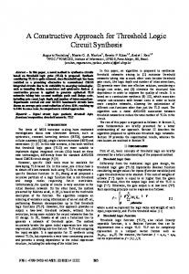
We use our region tracking algorithm proposed in [20] to extract the field lines from the images. We determine the boundary of all green regions in the images and we search for green-white-green transitions, perpendicular to the boundary curves. Figure 2 illustrates this process for the omnidirectional images we use. After having extracted the lines they are represented by the pair (P, C) where P = p0 , ..., pn−1 is a set of n points with cartesian x,y-coordinates and C = c0 , ..., cl−1 supplies connectivity information that partitions P into l point sequences. Here each ci = (si , ei ) is a tuple of indices determining the start and end point in P that belong to the corresponding point sequence. That is, point sequence i consists of the points psi , ..., pei . By manipulating the connectivity information C, point sequences can be split or merged. The line contours as illustrated in figure 2 b) are distorted due to the mirror in the omnidirectional vision system. In the following we assume that the distortion has been compensated. However, even without removing the distortion correctly, we are still able to detect most of the features. Fig.3 can provide an impression of the initial data. In many cases, there are long point sequences that correspond precisely to the shape of the field lines. However, there are also outliers, missing lines, and small line fragments due to occlusion and detection errors.
3
The feature construction process
In this section, we describe how features are detected in line contours. The overall detection process is performed in several steps which iteratively construct higher features from the components of prior steps. The input for the first step are the line contours extracted from the images.
(a)
(b)
Fig. 2. (a) A local line detector is applied along the boundaries of the tracked regions. (b) The resulting line contours consist of a set of lines, where each line is represented by a sequence of points which are marked by small circles.
3.1
Splitting the lines
Field lines consist of curved and straight lines. We want to classify the perceived line contours into these two categories. However, the initial contours often consist of concatenated curved and straight segments. To classify them separately we have to split the lines at the junctions. Junctions coincide with points of local maximum curvature. We retrieve them by first calculating a curvature measure for each point and then finding the local maxima. Although there exist sophisticated methods to calculate curvature (see for instance [2]), we have adopted a very simple approach for the sake of efficiency. For each point we consider two more points, one before and one after the current point. With these three points we compute two approximative tangent vectors, one reaching from the left to the midpoint and one from the midpoint to the right point. Finally, we define the curvature at the midpoint to be the angle by which the first vector has to be rotated to fall on the second. In order to be resilient against local noise in the curvature, we choose the enclosing points some distance from the midpoint. Since all the points are approximately equally spaced, we can afford to use an index distance instead of a precise geometric distance. That is, for a point p[i] at index i we choose the enclosing points to be p[i − w] and p[i + w] (w = 4 in our implementation). At the beginning and end of each line, we continually decrease w in order to be able to calculate the curvature. For the first and last point, the curvature is not defined. To detect local maxima of the curvature measure, we have adopted the following approach: While traversing the curvature values we detect intervals of values which exceed a given threshold and within each interval, we determine the index with the maximal value. To avoid extrema too close together, a new
Fig. 3. Four examples of extracted line contours. Some long sequences of points correspond precisely to the shape of the field lines. But there are also outliers, missing lines, and small line fragments due to occlusion and detection errors.
interval is opened only if it is at least at some given distance from the previous interval. Figure 4 shows the locations found for split points for various lines. Splitting can be performed efficiently by modifying the connectivity information in C (see section 2). 3.2
Classification
After the point sequences have been split, we classify each split sequence either straight or curved, applying the following test criterion: Similarly as for the curvature measure, we determine the angle between two vectors, but this time those defined by the first, the mid and the last point of the current point sequence. If the absolute value of the angle exceeds a threshold tφ (tφ = 0.4 radians in our application), then the point sequence is declared to be curved, otherwise
Fig. 4. Some examples that demonstrate the location of the split points.
straight. Independently of the actual choice of tφ wrong classifications can occur. However, the overall detection process can cope with a limited number of erroneous classifications. 3.3
Constructing arcs and straight lines
For each straight point sequence a line is constructed taking the respective start and end point. Similarly, a circular arc is constructed for each curved point sequence: The start point, the midpoint and the end point define two segments whose perpendicular bisectors intersect at the center of the circular arc. In order to verify, whether the points really form an arc, we calculate the mean deviation of the points from the arc’s radius and discard the arc if the distance is above the threshold trad = 0.03. In order to allow larger arcs to have a larger deviation, we divide the mean deviation by the radius before testing against the threshold. 3.4
Grouping arcs and detecting the center circle
Circular arcs which emerge from the same circle have centers which are close together. In order to group them, we search for clusters of the center points of the arcs. We apply the following cluster algorithm: Initially we have no clusters. The first cluster center is set at the center of the first arc. Then, we traverse the remaining arcs, and calculate the respective distance of their centers to the cluster centers. We choose the closest existing cluster and verify the distance. If it exceeds half of the actual arc’s radius, we start a new cluster at the respective position. Otherwise, we adapt the cluster center to represent the weighted mean position of all assigned arc’s centers. Here, the weights are the lengths of the arcs, which we approximate by the number of points of the point sequence from which the arc was constructed. We proceed in this way for all arcs and we obtain a set of clusters from which we choose the one with the greatest weight which reflects the number of assigned points. We demand, that at least 20 points have to be
assigned and that the radius should be approximately one meter (the radius of the center circle). If these conditions are met, we generate a hypothesis for the center circle which will be refined as described next. 3.5
Refining the center circle
The center circle was constructed from the arcs and the arcs where constructed from point sequences which were classified as curved. However, it happens often that point sequences which are part of the center circle are short and almost straight. Typically, they are classified as straight and no arcs are constructed from them. We want to include this data for the precise detection of the center circle. Thus, we traverse all straight point sequences and verify if they could be part of the initial hypothesis for the center circle. We verify the distance of the actual point sequence to the circle and whether the orientation of the point sequence fits the tangent direction of the circle, at the corresponding location. We allow some tolerance, since the initial hypothesis is not perfect. In this way we obtain a set of points, the points of the arcs and the points of misclassified straight lines which belong to the circle. Next, we refine the initial hypothesis of the circle using Landau’s method [12], a simple iterative technique which adjusts the center and the radius to the set of points. Typically, only few iterations (1-4) are required. Figure 5 illustrates this step. Later, we will search for the center line which passes through the circle in order to determine the corresponding orientation. 3.6
Determining the principal directions
Straight field lines of the playing field are either parallel or perpendicular. We want to determine the corresponding two orientations in the extracted contours. We will refer to them as principal directions. We will determine them with the straight lines constructed previously. Typically, spurious straight lines are present and we apply a clustering algorithm to cope with the outliers. For each line i, we calculate its orientation φi , normalizing the orientation to lay within [0, ..., π]. Each line votes for the angles φi and φi + π/2. Here, we apply the same clustering method as for the center circle, but this time working on one-dimensional values. We open a new cluster if the angular difference to the best cluster exceeds 0.3 radians. Otherwise, the cluster center is adjusted, with the weights being the lengths of the contributing lines. Finally, the cluster with the greatest weight determines the first principal direction ψ0 . The second principal direction ψ1 equals the first, rotated by 90 degree. In the following sections we will consider two lines through the origin having the direction ψ0 and ψ1 , respectively. We will refer to these lines as the principal axis a0 and a1 . Figure 6a) shows an example. 3.7
Discarding unreliable and grouping collinear lines
Having determined the main axis’ a0 and a1 we consider three types of lines. Those which are perpendicular to a0 , those which are perpendicular to a1 , and
(a)
(b)
Fig. 5. The position and radius of the initial circle is refined. Points which are considered to originate from the circle are shaded. Initially (a), only the points of curved point sequences are considered to be part of the circle. Thus, the initial circle is not optimal. In (b) additional points have been determined by identifying point sequences which are close to the initial circle. The initial circle is iteratively adjusted to the points by Landau’s method [12]. Only few iterations are required (two iterations in this example).
those whose orientation differs from both ψ0 and ψ1 by more than 0.3 radians. We consider the latter lines unreliable and discard them. The following step is performed for both a0 and a1 together with the respective perpendicular lines. Therefore, we will write a instead of a0 and a1 in the following. Let L = {l0 , l1 , ..., ln } denote the set of lines li which are perpendicular to a. Furthermore, let mi be the mid point of line li . We consider the orthogonal projections of all mi onto the axis a. Lines which are collinear will yield close projection points. Since a passes through the origin, each projection point of mi can be represented by a single value ti which is the distance of the projected point to the origin. Collinear lines will have the same values ti . However, since the lines are not precisely collinear, the ti will differ slightly. Thus, to find groups of collinear lines which are perpendicular to a we search for clusters of the ti . Again, we apply the same clustering algorithm described for the circle detection and the determination of the principal directions. A new cluster is opened if the distance to an existing cluster is greater than 20 centimeters. Each cluster, stores the lines which were assigned to it. Thus, each cluster represents a group of collinear lines which are perpendicular to the respective main direction. The lines within each group are replaced by a single line which encompasses the full range of the original lines. Finally, we sort the groups by their one-dimensional cluster centers tj . Note, that the difference tj − tk of two groups of parallel lines is just the distance between the lines. By sorting for tj , we obtain a topological order of the groups of collinear lines which will be very useful for the detection of
(a)
(b)
Fig. 6. The original line contours are painted gray. In (a) the straight lines are drawn by black arrows and the principal axis’ found are shown. Discarded straight lines are drawn in gray. The results of grouping the lines into collinear sets are shown in (b). The dashed thin lines reflect the groups. Each group is simplified by a single line. The order of the groups is shown by numbers.
the penalty area and the corresponding corners. Figure 6b) illustrates the results of this processing step. 3.8
Detecting the corners of the penalty area
The rectangle marking the goal area, and the rectangle marking the penalty area produces three lines parallel to the baseline. The lines are spaced at a distance of 50 and 100 centimeters. Having grouped and sorted the sets of collinear lines, we can easily detect such a structure. Here, we allow a tolerance of 20 centimeters when verifying the distances. Note, that the structure emerges at the start or end of the sequence of sorted collinear line groups, since the lines are the outmost existing lines. Having detected such a structure, the direction towards the goal is now known. Thus, we can distinguish between the left and right side of the lines. In order to find the respective corners, we simply verify whether we find perpedicular lines whose endpoints are close to the given lines. Some additional constraints have been necessary in order to avoid spurious detections. First, if we find three parallel lines that have the given structure in their distances, we calculate the overall length of the structure, in the direction of the lines. This length should not exceed the length of the penalty area, which is 5 meters. We allow a tolerance of 50 centimeters. A second constraint is that no lines which are perpendicular to the three lines are beyond the goal line.
4
Experimental results
This section describes our experimental results. Feature detection is influenced by many factors: By the preprocessing step which extracts the field lines, by line occlusions, by the region tracking algorithm, by the geometrical distortion calibration and on the lighting conditions. We tried to focus on the main situations. In order to test the influence of different environments we examined two different playing fields. The first with a green carpet and artificial lighting, the second with a reflecting linoleum floor, with natural light shining from one side through an array of windows. However, since the reflections on the floor where almost white in the images, we reduced the influence of natural light by adding artificial light from above and using venetian blinds. However, we did not shut the blinds completely. On both playing fields, we let the robot automatically move on a trajectory forming an eight (see figure 7). Localization was achieved using odometry and the recognized features, which yield unique robot poses, up to the symmetry of the playing field. On both fields, the robot did not loose its position. After 10-20 minutes we stopped the experiment. Moreover, when the robot was manually transferred to an unknown position, the robot immediately found its correct position after perceiving a feature. The maximum positional error while driving was about 20 cm.
Fig. 7. The path shows a robot moving on the field along a predefined figure. As can be seen, the maximum deviation is lower than 20 cm for a robot driving 0.8 m/s.
While the robot moved, we logged all the extracted line contours in a file and later, we manually verified the feature recognition for all frames. On both fields not a single false positive was detected. However, there are situations when features are not recognized. The corners of the penalty area cannot be detected, if an obstacle is occluding the corner. That is, the system does not infer the intersection point of two perpendicular lines, but rather demands that the endpoints of two lines are close together. Here, some improvements might be possible, however one must take care, not to infer corners which do not exist. However, all four corners will be rarely occluded at the same time. With our robot, which has a very low mirror and thus, has a limited range of sight, the robot can typically not detect the corners in a distance greater than 3 meters. However, during attack and defense when the robots are near the penalty area, at least one of the corners can be seen most of the time. The recognition of the center circle is possible up to a distance of approximately 3 meters, using our robots. We have some astonishing situations, where the center circle is still detected, although large parts are occluded by obstacles. This is possible, because a single fragment of a curved line can yield a hypothesis for the circle, which is then verified. However, if not a single curved line is found, the center circle is not detected. This typically occurs, when the center circle is distant to the robot, and when the correction of the optical distortion becomes imprecise. Then the splitting procedure tends to split noisy curved lines into many small straight fragments. At this point, further improvements are certainly possible. However, the important point is, that no false positives are detected. Also, note that it is not necessary to detect the features in every frame. Although the current system is able to run the recognition on every frame with 15 fps, this not necessary. It suffices, to perform the recognition, say every 10th frame, since the features yield very strong position clues.
5
Conclusion
We have proposed a method for detecting the center circle and four different types of corners in the neighborhood of the penalty area. Each of these features allows to localize the robot, up to the symmetry of the playing field. The method is robust and efficient and we have tested it thoroughly. Also, we have presented a general framework for feature construction. It should be possible to easily extend the approach to detect other features, such as the corner circle sectors of the playing field, for instance. Detected arcs, groups of straight lines, and the main directions are already available and it should be possible to construct different features from them. We hope that the palette of features will be extended continually by other researchers. Also, the individual algorithm can be improved or extended. In our approach we have used the region tracking algorithm described in [20]. However, maybe more efficient methods can be found that extract chains of points, representing the field lines. Here again, adaptivity to the illumination is the primary difficulty.
References 1. M. D. Alder. Inference of syntax for point sets. In E. S. Gelsema and L. N. Kanal, editors, Pattern Recognition in Practice IV, pages 45–58. New York: Elsevier Science, 1994. 2. H. Asada and M. Brady. The curvature primal sketch. In Proc. 2nd IEEE Workshop Computer Vision: Representation and Control, pages 8–17, 1984. 3. T.M. Breuel. Fast recognition using adaptive subdivisions of transformation space. In Proceedings. 1992 IEEE Computer Society Conference on Computer Vision and Pattern Recognition (Cat. No.92CH3168-2), pages 445–51, 1992. 4. R. N. Daves and K. Bhaswan. Adaptive fuzzy c-shells clustering and detection of ellipses. IEEE Transactions on Neuronal Networks, 3(5):643–662, 1992. 5. R.N. Daves. Fuzzy shell-clustering and applications to circle detection in digital images. International Journal on General Systems, 16:343–355, 1990. 6. Martin A. Fischler and Robert C. Bolles. Random sample consensus: a paradigm for model fitting with applications to image analysis and automated cartography. Communications of the ACM, 24(6):381–395, 1981. 7. A. Fitzgibbon and R. Fisher, 1995. 8. A. W Fitzgibbon, M Pilu, and R. B Fisher. Direct least square fitting of ellipses. IEEE Transactions on Pattern Analysis and Machine Intelligence, 21(5):476–480, 1999. 9. Gerd Mayer Hans Utz, Alexander Neubeck and Gerhard Kraetzschmar. Improving vision-based self-localization. Gal A. Kaminka, Pedro U. Lima and Ra´ ul Rojas (eds): RoboCup-2002: Robot Soccer World Cup VI, Springer, 2002. 10. P. V. C. Hough. Method and means for recognizing complex patterns. US Patent 3,069,654, December 1962. 11. Euijin Kim, Miki Haseyama, and Hideo Kitajima. Fast and robust ellipse extraction from complicated images. 12. U M Landau. Estimation of a circular arc center and its radius. Comput. Vision Graph. Image Process., 38(3):317–326, 1987. 13. Feng Lu and Evangelos Milios. Robot pose estimation in unknown environments by matching 2d range scans. CVPR94, pages 935–938, 1994. 14. R. A. McLaughlin and M. D. Alder. Recognising cubes in images. In E. S. Gelsema and L. N. Kanal, editors, Pattern Recognition in Practice IV, pages 59–73. New York: Elsevier Science, 1994. 15. R. A. McLaughlin and M. D. Alder. The Hough Transform versus the UpWrite. IEEE Transactions on Pattern Analysis and Matchine Intelligence, 20(4):396–400, 1998. 16. C. Olson, 2001. 17. Corneliu Rusu, Marius Tico, and Pauli Kuosmanen. Classical geometric approach to circle fitting - review and new developments. Journal of Electronic Imaging, 12(1):179–193, 2003. 18. Erik Schulenburg. Selbstlokalisierung im Roboter-Fußball unter Verwendung einer omnidirektionalen Kamera. Master’s thesis, Fakult¨ at f¨ ur Angewandte Wissenschaften, Albert-Ludwigs-Universit¨ at Freiburg, 2003. 19. Sebastian Thrun, Dieter Fox, and Wolfram Burgard. Monte carlo localization with mixture proposal distribution. In AAAI/IAAI, pages 859–865, 2000. 20. F. v. Hundelshausen and R. Rojas. Tracking regions and edges by shrinking and growing. In Proceedings of the RoboCup 2003 International Symposium, Padova, Italy, 2003.