A Data Clustering and Streamline Reduction Method for 3D MR Flow

A Data Clustering and Streamline Reduction Method for 3D MR Flow Vector Field Simplification Bernardo S. Carmo1 , Y.H. Pauline Ng2 , Adam Pr¨ ugel-Bennett1 , and 2 Guang-Zhong Yang 1

2

Department of Electronics and Computer Science, University of Southampton, SO17 1BJ, UK {b.carmo, apb}@soton.ac.uk Department of Computing, Imperial College London, 180 Queen’s Gate, London SW7 2BZ, UK {yhpn, gzy}@doc.ic.ac.uk

Abstract. With the increasing capability of MR imaging and Computational Fluid Dynamics (CFD) techniques, a significant amount of data related to the haemodynamics of the cardiovascular systems are being generated. Direct visualization of the data introduces unnecessary visual clutter and hides away the underlying trend associated with the progression of the disease. To elucidate the main topological structure of the flow fields, we present in this paper a 3D visualisation method based on the abstraction of complex flow fields. It uses hierarchical clustering and local linear expansion to extract salient topological flow features. This is then combined with 3D streamline tracking, allowing most important flow details to be visualized. Example results of the technique applied to both CFD and in vivo MR data sets are provided.

1

Introduction

Blood flow patterns in vivo are highly complex. They vary considerably from subject to subject and even more so in patients with cardiovascular diseases. Despite the importance of studying such flow patterns, the field is relatively immature primarily because of previous limitations in the methodologies involved in acquiring and calculating expected flow details. The parallel advancement of MRI and CFD has now come to a stage that their combined application allows for a more accurate and detailed measurement of complex flow patterns. Velocity Magnetic resonance imaging was originally developed in the mid 1980’s [1,2] and is now available on most commercial scanners. The accuracy of the method has been validated for the quantification of volume flow and delineation of flow patterns. There are now a wide range of clinical applications in acquired and congenital heart disease as well as general vascular disease. Computational fluid dynamics, on the other hand, involves the numerical solution of a set of partial differential equations (PDEs), known as the Navier C. Barillot, D.R. Haynor, and P. Hellier (Eds.): MICCAI 2004, LNCS 3216, pp. 451–458, 2004. c Springer-Verlag Berlin Heidelberg 2004


452

B.S. Carmo et al.

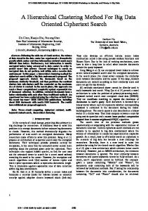
Fig. 1. Different flow field visualisation methods. (a) Arrow plot. (b) Interactive isovorticity plot. (c) Streamline plot.

Stokes (N-S) equations. The application of CFD has become important in cardiovascular fluid mechanics as the technique has matured in its original engineering applications. Moreover, with the parallel advancement of MR velocity imaging, their combination has become an important area of research [3]. The strength of this combination is that it enables subject-specific flow simulation based on in vivo anatomical and flow data [4]. This strategy has been used to examine flows in the left ventricle [5], the descending aorta, the carotid and aortic arterial bifurcation [6], aortic aneurysms and bypass grafts. With the availability of a detailed 3D model capturing the dynamics of the LV and its associated inflow and outflow tracts, it is now possible to perform patient specific LV blood flow simulation. For many years, techniques based on CFD have been used to investigate LV flow within idealised models. The combination of CFD with non-invasive imaging techniques has proven to be an effective means of studying the complex dynamics of the cardiovascular system as it is able to provide detailed haemodynamic information that is unobtainable by using direct measurement techniques. With the increasing use of combined MRI/CFD approach, the amount of data needs to be interpreted is becoming significant and becomes challenging to analyse and visualise (Figure 1). This is true especially when flow in major cardiac chambers through the entire cardiac cycle needs to be simulated. To examine detailed changes in flow topology, data reduction based on feature extraction needs to be applied. Streamlines give a good indication of the transient pattern of flow [7]. However, for 3D datasets these plots can be highly cluttered and for complex flow they tend to intertwine with each other, limiting their practical value [8]. The purpose of this paper is to present a new method for velocity MR flow field visualisation based on flow clustering and automatic streamline selection. Flow clustering enables data simplification and compression. The method assumes linearity around critical points to ensure that these are preserved by the simplification process. Each cluster therefore contains points sharing a common flow feature. Automatic streamline selection is then applied to determine the salient flow features that are important to the vessel morphology.

A Data Clustering and Streamline Reduction Method

2 2.1

453

Materials and Methods Clustering

Several methods based on hierarchical clustering have been proposed in recent years. Current methods can be divided into two categories: top-down [9] and bottom-up strategies [10,11] strategy. More recently, Garcke et al. [12] have proposed a continuous clustering method for simplifying vector fields based on the Cahn-Hilliard model that describes phase separation and coarsening in binary alloys. In general, all these methods use a single vector to represent a cluster and are well suited for visualisation purposes, however, given a set of such clusters, it is difficult to recover the original vector field. To generate an abstract flow field from a dense flow field, the dense flow field is partitioned into a set of flow regions each containing a cluster of vectors. Local linear expansion is employed to represent the clustered flow vectors. Using gradients to represent a flow field is particularly suitable for regions near critical points, and thus this representation technique intrinsically preserves critical points. A hierarchical clustering algorithm merges flow vectors in an iterative process. The fitting error, E(C), for each cluster C is defined as the total square distance between the original data points and the those fitted by the gradients. The cost MC of merging two clusters, C1 and C2 , to form a new cluster Cnew is: MC (C1 , C2 ) = E(Cnew ) − [E(C1 ) + E(C2 )] .

(1)

Initially, each vector forms its own cluster and the neighbouring vectors are used to approximate the local linear expansion of this cluster. Subsequently, the associated cost of merging a pair of clusters is calculated and stored in a pool for each pair of neighbouring clusters. The following steps are then repeated until all clusters are merged to form one single cluster enclosing the entire flow field. First, the pair of clusters with the smallest merging cost in the pool is removed and merged to form a new cluster. Then, the cost of merging the latter with its neighbours is calculated and inserted into the pool. By repeatedly merging clusters, a hierarchical binary tree is constructed in the process, with each node representing a cluster and its children representing its sub-clusters. Once the hierarchical tree is constructed, abstract flow fields at various clustering levels can then be obtained from this tree efficiently. 2.2

Local Linear Expansion

The flow field near critical points is assumed here to be linear. In order to enclose regions around critical points, each cluster joins points with approximately the same velocity gradients. Local linear expansion is carried out to determine these gradients inside each cluster.

454

B.S. Carmo et al.

We assume that the velocity in a region, R, is given by v = A(x − x0 ) = A x − v0

(2)

where v0 = A x0 . We know the velocity v at a set of cluster points. We therefore perform a
N least squares fitting over the lattice points in each cluster’s region R = x(i) i=1 , where x(i) designates the coordinates of each cluster point, and N is the size of the cluster. Least squares is equivalent to minimising the energy  1  v(i) − Ax(i) + v0 2 . (3) E= N i=1 where v(i) = v(x(i)) (i.e. the value of the velocity at the cluster point x(i)). Optimising with respect to v0 we obtain     (4) v0 = A x − v ,   where · · · denotes averaging over the points in the cluster. Substituting the optimal value of v0 into the energy and differentiating with respect to A, we can compute A using A = WT V−1 where

(5)

    T 1  x(i) − x v(i) − v N i=1     T 1  x(i) − x x(i) − x V= . N i=1

W=

To be able to reconstruct the flow field, we store v0 and the contents of A for each cluster. Retrieving the field’s velocities then simply involves applying equation (2). 2.3

Topology Display

Streamlines are generated in the same way as steady flow streamlines, but they must be interpreted as transient in time as they do not result from steady flow. Used in conjunction with clustering, however, they can be used to convey the overall topology of the field. After clusters have been formed from the flow field, streamlines are grown from equally spaced points throughout the image and stored in a streamline array. Each streamline passes through one or several clusters, and this is recorded in a list. A streamline “correlation” matrix Ccluster is then built by computing the ratio between common clusters occupied by streamlines and the total number of clusters spanned by each streamline: τcluster (e, v) Ccluster (e, v) = (6) γcluster (e)

A Data Clustering and Streamline Reduction Method

455

where e, v are streamline array indices, τcluster (e, v) is the number of clusters occupied by both e and v and γcluster (e) is the total number of clusters occupied by streamline e. The most representative streamlines can then be selected by setting a maximum streamline correlation Tcluster (e), the value of which is interactively chosen by the user. This is defined as: Tcluster (e) =

N 

Ccluster (e, v)

(7)

v=1 v
=e

where N is the total number of streamlines in the streamline array.

3

Results and Discussions

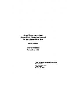
The proposed method was applied to 3D flow through the human heart simulated from a CFD model [13]. The model after mesh processing contained 54,230 nodes and 41,000 cells. A total of 16 meshes representing the LV across the complete cardiac cycle were generated from the original image data. In order to permit CFD simulation, it was necessary to increase the temporal resolution of the model. This ensured that none of the constituent cells underwent excessive deformation or displacement between adjacent time steps. To this end, cubic spline interpolations were performed to generate a total of 49 meshes across the cardiac cycle. The Navier-Stokes equations for 3D time-dependent laminar flow with prescribed wall motion was solved using a finite-volume based CFD solver CFX4 (CFX international, AEA technology, Harwell). The blood was treated as an incompressible Newtonian fluid with a constant viscosity of 0.004 Kg/(ms). The simulation was started from the beginning of systole with the pressure of the aortic valve plane set to zero and with the mitral valve plane treated as a non-slip wall. At the onset of diastole, the aortic valve was closed by treating it as a solid wall, whilst the mitral valve was opened by using a combination of pressure and flow boundaries. As can be seen in Figure 2, the choice of the maximum total correlation is important for the rendering result. If that value is too low, this results in too few streamlines being selected and flow features being missed (Figure 2(c)); if the value is too high, the display is cluttered by excessive streamlines (Figure 2(a)). This visualisation method was also applied along the time series data of the same dataset. The previous results depict the flow during diastole showing flow through the mitral valve, as shown in Figure 3. The proposed method was also applied to 2D in vivo MR velocity data acquired with sequential examination following myocardial infarction using a Marconi whole body MR scanner operating at 1.5T. Cine phase contrast velocity mapping was performed using a FEER sequence with a TE of 14ms. The slice thickness was 10mm and the field of view was 30-40cm. The dataset has a temporal resolution of 45ms and the diastolic phase is covered in about 5-10 frames, five of which are shown here.

456

B.S. Carmo et al.

Fig. 2. Effect of interactively changing the maximum total correlation threshold. (a) No threshold - all streamlines selected. (b) Tcluster (e)M AX = 20; (c) Tcluster (e)M AX = 10; (d) Tcluster (e)M AX = 5, the smaller vortex is now invisible.

Fig. 3. Simplified streamline rendering of 3D simulated flow inside the human cardiac left ventricle. Time samples 9 to 16 of a set of 33.

The dataset was denoised using the restoration scheme described in [14]. Figure 4 shows a comparison between our automatically selected streamlines and arrow plots overlayed on the corresponding conventional MR images. In order to quantify the error introduced by the clustering process we measured the rootmean-square difference between the original velocity field and that reconstructed by the cluster gradients using equation (2). The results are plotted in Figure 5 for clustering of the 12th frame (540ms) of the 2D in vivo dataset and time sample 12 of the 3D simulated dataset. The number of clusters used to produce all streamline plots in this paper was 10 for both datasets. The size of the region of interest was 3536 pixels and 47250 voxels for the 2D and 3D datasets, respectively.

A Data Clustering and Streamline Reduction Method

457

Fig. 4. Flow pattern within the left ventricle of a patient following myocardial infarction, from 450ms to 630ms after onset of ECG R wave, depicting vortical flow rendered by streamlines selected by clustering (top row) and 2D arrows where arrow size is proportional to velocity magnitude (bottom row). A 3-spaced grid was used to select the arrow data.

Fig. 5. Root mean square error between original and cluster velocity predicted from gradients (see text) for the 2D frames of Figure 4 (left) and 3D simulated time samples of Figure 3 (right).

4

Conclusion

We have presented a novel method for velocity MR flow simplification and display. Flow simplification is achieved by clustering, where each cluster contains points with similar local linear approximation gradients. This ensures that each cluster encloses points sharing relevant flow features. Streamlines are then generated over the flow field and selected using a measure of inter-streamline cluster overlap, interactively thresholded. The rendered streamlines depict the important features of the flow and present the observer with an overview of the general flow topology of the field. Acknowledgements. BSC is supported by a Portuguese FCT grant and a British EPSRC grant. YHPN is funded by the Croucher Foundation in Hong Kong.

458

B.S. Carmo et al.

References 1. van Dijk, P.: Direct cardiac NMR imaging of heart wall and blood flow velocity. J Comput Assist Tomogr 1984; 8: 429-36. 2. Bryant, D.J., Payne, J.A., Firmin, D.N., Longmore, D.B.: Measurement of flow with NMR imaging using a gradient pulse and phase difference technique. J Comput Assist Tomogr 1984; 8: 588-93. 3. Papaharilaou, Y., Doorly, D.J., Sherwin, S.J., Peiro, J., Anderson, J., Sanghera, B., Watkins, N., Caro C.G.: Combined MRI and computational fluid dynamics detailed investigation of flow in a realistic coronary artery bypass graft model, pp 379 Proc. Int. Soc. Mag. Res. Med. 2001. 4. Gill, J.D., Ladak, H.M., Steinman, D.A., Fenster, A.: Accuracy and variability assessment of a semi-automatic technique for segmentation of the carotid arteries from 3D ultrasound images. Med Phys 2000;27:1333-1342. 5. Saber, N.R., Gosman, A.D., Wood, N.B., Kilner, P.J., Charrier, C. L., Firmin, D. N.: Computational flow modelling of the left ventricle based on in vivo MRI data - Initial experience. Annals Biomed Engineering 2001; 29:275-283. 6. Long, Q., Xu, X.Y., Ariff, B., Thom, S.A., Hughes, A.D., Stanton, A.V.: Reconstruction of blood flow patterns in a human carotid bifurcation: A combined CFD and MRI study. JMRI 2000; 11:299-311. 7. Yang, G. Z., Kilner, P. J., Mohiaddin, R. H., Firmin, D. N.: Transient streamlines: texture synthesis for in vivo flow visualisation. Int. J. Card. Imag. 16: 175-184, 2000. 8. Interrante, V., Grosch C.: Strategies for effectively visualizing 3D flow with volume LIC. Proc. Visualization ’97 421-424, 1997. 9. Heckel, B., Weber, G., Hamann, B., Joy, K.I: Construction of vector field hierarchies. Proc. IEEE Visualization’99, 19-25, October 1999. 10. Telea, A., van Wijk, J.: Simplified representation of vector fields. IEEE Visualization 1999: 35-42. 11. Lodha, S.K., Renteria, J.C., Roskin, K.M.: Topology preserving compression of 2D vector fields. Proc. IEEE Visualization’00, 343-350, October 2000. 12. Garcke, H., Preußer, T., Rumpf, M., Telea, A., Weikard, U., van Wijk, J.J.: A phase field model for continuous clustering on vector fields. IEEE Trans. Visualization and Computer Graphics, 7(3): 230-241, 2001. 13. Long, Q., Merrifield, R., Yang, G.Z., Kilner, P.J., Firmin, D.N., Xu, X.Y.: The influence of inflow boundary conditions on intra left ventricle flow predictions. J Biomech Eng. 2003 Dec;125(6):922-7. 14. Ng, Y.H.P., Yang, G.Z.: Vector-valued image restoration with application to magnetic resonance velocity imaging. Journal of WSCG 11(2): 338-345, 2003.