Dipartimento di Scienze Economiche, Matematiche e Statistiche Università degli Studi di Foggia ____________________________________________________________________
A Data Set Generation Algorithm in Combinatorial Auctions Crescenzio Gallo Giancarlo De Stasio Cristina Di Letizia Quaderno n. 1/2006
Quaderno riprodotto al Dipartimento di Scienze Economiche, Matematiche e Statistiche nel mese di gennaio 2006 e depositato ai sensi di legge Authors only are responsible for the content of this preprint.
_______________________________________________________________________________ Dipartimento di Scienze Economiche, Matematiche e Statistiche, Largo Papa G. Paolo II, 1, 71100 Foggia (Italy), Phone +39 0881-75.37.28, Fax +39 0881-77.56.16
A Data Set Generation Algorithm in Combinatorial Auctions∗ Crescenzio Gallo (
[email protected]) Giancarlo De Stasio (
[email protected]) Cristina Di Letizia (
[email protected]) Dipartimento di Scienze Economiche, Matematiche e Statistiche Universit`a di Foggia Largo Papa Giovanni Paolo II, 1 - 71100 Foggia (Italy)
Abstract The generation of realistic data sets in a Combinatorial Auction may be a challenging problem. Well-formed data sets are very useful in the evaluation of algorithms trying to solve the winner determination problem. In this paper a general data set generation scheme is presented, both from an algorithmic and economic point of view. As a case study, a possible auction setting is discussed where the goods on sale are connections between points in space. JEL classification: C51, C61, C87, C99. Keywords: bid, combinatorial auction, data set generation.
∗
A previous version has been accepted as a contributed paper at the IEEE EUROCON 2005 Conference. The usual disclaimers apply.
1
Contents 1
I NTRODUCTION
3
2
E CONOMIC PARAMETERS IN R EALISTIC CA S 2.1 Bidders number . . . . . . . . . . . . . . . . 2.2 Items number . . . . . . . . . . . . . . . . . 2.3 Items value . . . . . . . . . . . . . . . . . . 2.4 Bidders’ size . . . . . . . . . . . . . . . . . 2.5 Operational indications . . . . . . . . . . . .
4 4 4 5 5 6
. . . . .
. . . . .
. . . . .
. . . . .
. . . . .
. . . . .
. . . . .
. . . . .
. . . . .
. . . . .
. . . . .
3
B ID G ENERATION IN S TRUCTURED D OMAINS
6
4
G ENERATING R EALISTIC DATA S ETS 7 4.1 Railroad network generation . . . . . . . . . . . . . . . . . . . . 8 4.2 Bid Generation . . . . . . . . . . . . . . . . . . . . . . . . . . . 11 4.3 Algorithm “Bid Generation” . . . . . . . . . . . . . . . . . . . . 12
5
F URTHER W ORK
12
References
13
List of Figures 1 2
Generation of the railroad network . . . . . . . . . . . . . . . . . 9 Node valuation by iterated powers method . . . . . . . . . . . . . 11
2
1
I NTRODUCTION
C OMBINATORIAL AUCTIONS (CAs) are interesting both for Economics and Computer Science researchers. In a CA a bidder can place unrestricted bids, economically evaluating the combination of sets of items. With respect to a traditional auction, a bidder may take into account complementarities (i.e., V (A and B) ≥ V (A) + V (B), being V (X) the bidder’s valuation of good X on sale) and substitutabilities (i.e., V (A and B) ≤ V (A) + V (B)). This makes it possible to design auctions mechianisms that are economically more efficient. CAs seem to be well suited for problems such as airport time slots allocation (Rassenti and Bulfin (1982)), machine time scheduling (Wellman and MacKieMason (1998)), real estate (Quan (1994)), delivery routes (MIT (1996)). A number of technical problems have to be solved before unrestricted CAs can be used in practice. For n items on sale, a bidder can place an offer of any subset of interest, with up to 2n different bids for the auctioneer. Two issues are those of how to synthetically express a bid and how to communicate it to the auctioneer efficiently (see Nisan (2000)). Another fundamental problem is that of winner determination, aka the allocation problem: i.e., after receiving a set of (combinatorial) bids, decide how to allocate the goods in order to satisfy the constraints (a good to at most one bidder) and to maximize the total bid takers payoff. Although this is an NP-hard to approximate problem (Sandholm (1996), Vohra and de Vries (2001)), in practical cases the situation may be substantially better, leading various researchers to the proposition of polynomial time approximation algorithms (e.g. Zurel and Nisan (2001)): this paper aims to contribute in the experimentation of these theorical results with variable size data sets reflecting the characteristics of the real algorithms input data. As far as we know, the only attempt to provide a realistic suite for generating test sets is the work by Leyton-Brown and Shoham (2000), in which they consider a number of potential application areas for CAs and propose bid generation mechanisms that try to reflect the underlying structural as well economic factors, but probably overlooking a number of economic issues that would greatly help in the generation of realistic data sets. In this paper we concentrate on such economic 3
issues and devise some high level guidelines to generate realistic bids. In particular, in Section II the properties of goods at auction and those of the bidders are investigated, while in Section III a general scheme for bid generation in structured domains is discussed. Finally, we briefly mention directions for further work.
2
E CONOMIC PARAMETERS IN R EALISTIC CA S
Let S denote the set of items on sale and let I = |S| be the cardinality of the set S. Also, let B denote the set of bidders submitting bids to the auctioneer. Here we analyze the parameters B and I that characterize realistic auction settings, and the distribution of the value of items and size of bidders.
2.1
Bidders number
The parameter B can vary greatly if bidders are firms instead of individuals. In the case of firms, substantially B ≤ 100; in a typical business-to-consumer auction, instead, B can be up to 10, 000 (if, for example, we consider an auction taking place over the Internet). A more interesting measure is the number of bidders relative to I, reasonably being B/I ≤ 10, with the special cases B/I = 1, 2 interesting for most economic phenomena.
2.2
Items number
It ranges from a few dozens (in auctions involving consumer products or complex industrial items, such as spectrum frequencies or intermediate goods), to a few hundreds (in auctions involving a long list of heterogeneous products, such as spare parts); there may also be auctions involving a large number of items (I >> 100), but in this case it is likely that the goods on sale are of quasi-homogeneous type.
4
2.3
Items value
It is likely that for any given item the bidder gives it a value close to its market value. If the average value is small, then it is conceivable that there are few items with comparatively large value (i.e., r = ”value of most expensive item” / ”value of less expensive item” >> 1). In this case, the actual values can be generated using a left skewed distribution, such as the log-normal or Pareto distribution. On the other hand, when the items have high values, it is more likely that the ratio r is bounded (r = 2 or r = 3); in this case the actual values can be generated using a symmetric distribution, such as the uniform or normal distribution. If the set of items on sale is structured, other considerations may apply as well. For instance, when the items are paths in space, which is our case study in Section IV, it is reasonable that the value of a path P may affect the value of paths that have points in common with P (e.g., the value of a side connection may depend on the value of the backbone connection which the side one originates from). In these cases, the market values may be generated using some sort of structural computations (as we shall see in Section IV).
2.4
Bidders’ size
For individual bidders the size is the income (and the value of items never exceeds it), while for companies is the total assets (with debt possible but excluded for financial markets limitations). In case of small value items, the size of bidders is usually not relevant (we assume unlimited budget); but if the ratio average bidder size / average item value tends to be small, then an important role is played by the size distribution function. Size, in general, follows a left skewed distribution, because both individual income and firm size are asymmetrically distributed (see Ijiri and H. Simon (1977)). In this case, it may be assumed a support 0 to 1 billion dollars for income and 0 to 100 billion dollars for assets. Once a left skewed distribution has been fixed, we only need to pick the distribution parameters in such a way that the ratio AS ( = average bidders’ size) / AV ( = average value of items) is of the desired value (and possibly inversely correlated to the number of auctioned items).
5
2.5
Operational indications
The above indications lead to the following general scheme for the generation of the item values and the size of bidders. 1. Fix the number of items. 2. Fix the ratio B/I to define the number of bidders. 3. Choose a distribution for the value of items. 4. If the size of bidders is relevant, choose a left skewed distribution for it. 5. Fix the distribution parameters of 3 and 4 in such a way that AS/AV is of the desired value. Let us consider, for example, the Pareto distribution. A random variable X has a Pareto distribution if its density function is given by f (X) = aX − (a + 1), with a > 1. For such random variable E(X) = a/(a − 1). Hence, if 3 and 4 are both Pareto, a and b are (respectively) the parameters for the firm size and item value distribution, and the desired ratio AS/AV = 2, then a and b must be chosen in such a way that [a/(a − 1)]/[b/(b−1)] = 2. Upon having chosen 3 and 4 (and fixed their parameters according to 5): 6. Generate a random sample of numbers from 3 and 4, with the sample size determined by 1 and 2.
3
B ID G ENERATION IN S TRUCTURED D OMAINS
In this section we sketch the general ideas for the generation of realistic bids in structured domains, i.e., when the goods on sale can be seen as the element of a space’ equipped (at least) with a distance function. These ideas will be made more precise in the next Section, where we address our case study. First of all, a bidder must be assigned a goal that she will pursue subject to her size (and hence budget) limitations. Clearly, goals are highly dependent on the nature and structure of the items on sale. As an example, if items can be
6
represented as the edges of a graph (as in the case study of Section IV), then a reasonable goal is that of acquiring a (simple) path joining two nodes. Once the goal has been fixed, the actual bids can be produced. For both goal generation and bidding a certain degree of randomness must be introduced to model the facts that: (1) different bidders may be interested in different sets of items, and that (2) different bidders can make different valuations of the same set of items. Let us consider the goal generation problem in more details. Let S be a subset of S; S should include the most valuable’ items in S. Each bidder selects a random subset of S and ranks all the elements in S according to their average distance from the elements in the random subset selected. Clearly, different bidders will have different rankings with high probability. Now, given a budget and a ranking of the items, we are able to generate a goal for a bidder as follows: we start by selecting the highest ranked item e and form a bid by adding as many items as possible among those close to e. Clearly, if e is too much expensive, we try with the next highest ranked item. Obviously, as pointed out at the beginning of this Section, much fine tuning is necessary as to precisely define the goal in a number of cases. Once the items to be included in the bid have been determined, the actual price offered is essentially the sum of their market values. However, the bidder’s valuation of a single item needs not coincide with its market value (generated according to the above scheme), as it also depends on subjective evaluations. Yet it is reasonable to regard the market value of an item as the indicative price an individual or a firm is willing to pay for that item. We can take subjective elements into account by simply perturbing the market value. As an example, we can generate bidder’s valuations by sampling from a (quite narrow) normal distribution with mean the market value. A similar approach (but possibly using a left skewed distribution) can be adopted to produce superadditive valuations of sets of items.
4
G ENERATING R EALISTIC DATA S ETS
In this section we specialize the economic parameters and the high level scheme of Sections II and III to the generation of realistic test sets for the allocation of
7
the rights to use railroad tracks. A railroad network is an example of a structured domain, and we will use the underlying properties to both assign values to the items on sale and to generate the bids. As in Leyton-Brown and Shoham (2000), the first step is the generation of the railroad map. We propose a different algorithm to generate families of graphs that, in our opinion, better reflects the way actual railroad networks have developed, i.e., by the merging of local and/or regional (or even national) networks, which were originally independent or very weakly interconnected.
4.1
Railroad network generation
Given an euclidean graph G, let the distance between two different connected components G1 and G2 of G be defined as the minimum, over all pairs (a, b) such that a ∈ G1 and b ∈ G2 , of the distances between a and b. The network generation algorithm is the following. 1. Randomly place n1 points on a square region and connect each point with its k closest neighbors. 2. Repeat the following: (a) check whether the graph is connected; (b) if connected, then go to 3; (c) make each connected component biconnected, and connect each (bi) connected component with the component at minimum distance; (d) goto 2a. 3. Make the graph biconnected. 4. Randomly place n2 points. 5. Connect each new point with its closest neighbor in the initial set of random points.
8
Figure 1: Generation of the railroad network
9
Fig. 1 illustrates the process of construction of an example railroad network, with parameters n1 = 13, k = 1, and n2 = 3, according to the above algorithm. The reason why we make each connected component biconnected is that a railroad network hardly contains articulation points, except possibly for nodes with degree 1 (which we add as the last step of our algorithm). Here the goods on sale are the edges of the network; however, the network generation algorithm presented above is parametrized by the number of nodes (i.e., cities) rather than edges. It is possible to prove that, when k = 1, the number of edges generated does not exceed 2n1 + n2 ≥ n1 + n2 = n (number of items). We will assume n1 ≤ 50 and n2 ≤ 10 with either k = 1 or k = 2; for the number of bidders, we shall fix B = min{2I, 100}. The rules according to which we assign market values to the items are the most crucial of the whole bid generation procedure. We begin by observing that the value of a train path depends on the expected number of passengers that travel on it in the unit of time. In turn, this depends on the importance of the nodes (cities) touched by that path. The value of a city does depend on external (with respect to the railway system) factors but also on the degree of the corresponding node and, in a recursive way, from the value of the nodes which is connected to. Hence we assign market values to the edges of the graph by first assign values to the nodes. After that, we assign an edge e = (c1 , c2 ) the value V (e) = [V (c1 ) + V (c2 )]d(c1 , c2 ), where V denotes the market value function (for both nodes and edges) and d(·, ·) denotes the euclidean distance. The problem is thus that of assigning values to the cities. Our approach is to assign to node i the value of the i-th component of the normalized eigenvector associated with the eigenvalue of maximum absolute value of the adjacency matrix of the graph. The argument (which is commonly used in different contexts, for instance to compute the authority weight of web sites (Kleinberg (1999)) is that the importance of a city is given by the importance of the cities it is connected to. If we ignore factors external to the railway systems, the value can then be computed by the iterated powers method applied to the adjacency matrix, and this can be easily proved to converge to the principal eigenvector. In Fig. 2 we show the values this method gives to the nodes (cities) of the example network of Fig. 1. 10
According to the general scheme of Section II, the size of bidders is generated using a left skewed distribution (either lognormal or Pareto). The average size can be taken (parametrically) up to ten times the average value of the items on sale.
Figure 2: Node valuation by iterated powers method
4.2
Bid Generation
The actual bid generation follows the general guidelines outlined in Section III. Let S denote the set of the first 10 to 20 most valuable edges of the graph. A bidder i randomly selects a subset Si of S of cardinality b|S|/hc, where h = 2, 3 typically. As already pointed out, Si will be used to rank all the edges in the graph. The rank of an edge is computed by calculating its average distance from the edges in Si ; here we define the distance between two edges e1 and e2 as the minimum distance in the graph between endpoints of e1 and e2 . The rank of an edge is then given by the rank of the corresponding average distance in the set of all the computed distances. Given a budget and an ordering of the edge set, a bidder formulates a bid according to the algorithm given below. We assume that the goal of the bidder is to get a set of edges of total length greater than a minimum required value, and 11
whose ranks are as highest as possible.
4.3
Algorithm “Bid Generation”
1. Select the next highest ranked edge (among those not yet considered). If the rank is below a given threshold, we assume failure for the current bidder. 2. Select a few other edges that form (together with the edge devised at step 1) a path in the graph. This path will form the “backbone of the bid. 3. Select a few edges that represent connections from and to the backbone. Each connection, together with the backbone, will form a separate bid. Clearly the bids are (implicitly) xor-ed, since they all share the backbone. The value associated to a bid is given by the sum of the bidder’s valuations of the edges included in the bid. These valuations are determined by slightly (and randomly) perturbing the market prices. 4. If the budget constraint is violated, step 3 is repeated. If this happens repeatedly, the algorithm goes back to step 1. 5. (Success) The value of the bid generated can be increased by a small random amount (not more than 10% of the value computed so far) as a function of the rank of the edges included. This can actually produce superadditive bids.
5
F URTHER W ORK
Currently we are implementing a suite for the generation of realistic data sets in structured domains. One such domain is the allocation of paths in space discussed in this paper (a different domain we are working with is real estate). The goal is to use this data to perform in-depth analyses of the performance of a number of approximation algorithms that have been proposed in the literature. A related goal is to get insights that will possibly help to devise more time-and-space-efficient allocation algorithms that closely approximate the optimum values on realistic data. 12
References Ijiri Y. and H. Simon H. (1977) Skew distribution and the sizes of business firms, North-Holland, Amsterdam. Kleinberg J. (1999) Authoritative sources in a hyperlinked environment, Journal of the ACM, 46, 604–632. Leyton-Brown K. P.M. and Shoham Y. (2000) Towards a universal test suite for combinatorial auction algorithms, in: Proc. of EC, 66–67. MIT (1996) An optimization based bidding process: a new framework for shippercarrier relationships, Thesis, Dept. of Civil and Environmental Engineering, School of Engineering. Nisan N. (2000) Bidding and allocation in combinatorial auctions, in: Proc. of EC. Quan D. (1994) Real estate auctions: a survey of theory and practice, Journal of Real Estate Finance and Economics, 9, 23–49. Rassenti S. S.V. and Bulfin R. (1982) A combinatorial auction mechanism for airport slot allocation, Bell Journal of Economics, 13, 402–417. Sandholm T.W. (1996) Limitations of the vickrey auction in computational multiagent systems, in: Proc. 2nd Int. Conf. on Multiagent Systems, 299–306. Vohra R. and de Vries S. (2001) Combinatorial auctions: A survey, Technical report, http://www.kellogg.nwu.edu/faculty/vohra/htm/res.htm. Wellman M. W.W.W.P. and MacKie-Mason J. (1998) Auction protocols for decentralized scheduling, in: Proc. 18th Int. Conf. on Distributed Computing Systems. Zurel E. and Nisan N. (2001) An efficient approximate allocation algorithm for combinatorial auctions, in: Proc. of EC.
13