A Distributed Monitoring Mechanism for Wireless Sensor Networks Chih-fan Hsin
Mingyan Liu
University of Michigan 1301 Beal Avenue, 4301EECS Ann Arbor, Michigan 48109
University of Michigan 1301 Beal Avenue, 4238 EECS Ann Arbor, Michigan 48109
[email protected]
[email protected]
ABSTRACT In this paper we focus on a large class of wireless sensor networks that are designed and used for monitoring and surveillance. The single most important mechanism underlying such systems is the monitoring of the network itself, that is, the control center needs to be constantly made aware of the existence/health of all the sensors in the network for security reasons. In this study we present plausible alternative communication strategies that can achieve this goal, and then develop and study in more detail a distributed monitoring mechanism that aims at localized decision making and minimizing the propagation of false alarms. Key constraints of such systems include low energy consumption and low complexity. Key performance measures of this mechanism include high detection accuracy (low false alarm probabilities) and high responsiveness (low response latency). We investigate the trade-offs via simulation.
Categories and Subject Descriptors C.2 [Computer System Organization]: Computer Communication Networks; C.3 [Computer System Organization]: Special-Purpose and Application-Based Systems; I.6 [Computing Methodologies]: Simulation and Modeling
General Terms Design, Performance, Security
Keywords wireless sensor networks, system design, security, monitor and surveillance
1.
INTRODUCTION
The rapid advances in wireless communication technology and micro-electromagnetic systems (MEMS) technology
Permission to make digital or hard copies of all or part of this work for personal or classroom use is granted without fee provided that copies are not made or distributed for profit or commercial advantage and that copies bear this notice and the full citation on the first page. To copy otherwise, to republish, to post on servers or to redistribute to lists, requires prior specific permission and/or a fee. WiSe’02, September 28, 2002, Atlanta, Georgia, USA. Copyright 2002 ACM 1-58113-585-8/02/0005 ...$5.00.
have enabled smart, small sensor devices to integrate microsensing and actuation with on-board processing and wireless communications capabilities. Due to the low-cost and small-size nature, a large number of sensors can be deployed to organize themselves into a multi-hop wireless network for various purposes. Potential applications include scientific data gathering, environmental monitoring (air, water, soil, chemistry), surveillance, smart home, smart office, personal medical systems and robotics. In this study, we consider the class of surveillance and monitoring systems used for various security purposes, e.g., battlefield monitoring, fire alarm system in a building, etc. The most important mechanism common to all such systems is the detection of anomalies and the propagation of alarms. In almost all of these applications, the health (or status of well-functioning) of the sensors and the sensor network have to be closely monitored and made known to some remote controller or control center. In other words, even when no anomalies take place, the control center has to constantly ensure that the sensors are where they are supposed to be, are functioning normally, and so on. In [10] a scheme was proposed to monitor the (approximate) residual energy in the network. However, to the best of our knowledge, a general approach to the network health monitoring and alarm propagation in a wireless sensor network has not been studied. The detection of anomalies and faults can be divided into two categories: the explicit detection and the implicit detection. An explicit detection occurs when an event or fault is directly detected by a sensor, and the sensor is able to send out an alarm which by default is destined for the control center. An example is the detected ground vibration caused by the intrusion of an enemy tank. In this case the decision to trigger an alarm or not is usually defined by a threshold. An implicit detection applies to when the event or intrusion disables a sensor from communication, and thus the occurrence of this event will have to be inferred from the lack of communication from this sensor. Following an explicit detection, an alarm is sent out and the propagation of this alarm is to a large extent a routing problem, which has been studied extensively in the literature. For example, [2] proposed a braided multi-path routing scheme for energy-efficient recovery from isolated and patterned failures; [4] considered a cluster-based data dissemination method; [5] proposed an approach for constructing a greedy aggregation tree to improve path sharing and routing. Within this context the accuracy of an alarm depends on the pre-set threshold, the
sensitivity of the sensory system, etc. The responsiveness of the system depends on the effectiveness of the underlying routing mechanism used to propagate the alarm. To accomplish implicit detection, a simple solution is for the control center to perform active monitoring, which consists of having sensors continuously send existence/update (or keep-alive) messages to inform the control center of their existence. Thus the control center always has an image about the health of the network. If the control center has not received the update information from a sensor for a prespecified period of time (timeout), it can infer that the sensor is dead. The problem with this approach is the amount of traffic it generates and the resulting energy consumption. This problem can be alleviated by increasing the timeout period but this will also increase the response time of the system in the presence of an intrusion. Active monitoring can be realized more efficiently in various ways. Below we discuss a few potential solutions. The most straightforward implementation is to let each sensor transmit the update messages at a same fixed rate. However, due to the multi-hop transmission nature and possible packet losses, this results in sensors far away from the control center (thus with more hops to travel) achieving a much lower goodput. This means that although updates are generated at a constant rate, the control center receives updates much less frequently from sensors further away. In order to achieve a balanced reception rate from all sensors the traffic load has to be kept very low, which means that the system must have a relatively low update rate. This approach then is obviously not suitable for systems that require high update rate (high alertness). Alternatively we could let each sensor adjust its update sending rate based on various information. For example, increase the sending rate if a sensor is further away from the controller (which would require the sensor to have knowledge on hop-count). [8] suggested adjustment based on channel environment, i.e., let sensors with higher goodput increase their sending rate and sensors with lower goodput decrease their sending rate. However, parameter tuning is likely to be very difficult and it is not clear if this approach is scalable. A second approach is to use inference and data aggregation. Suppose the control center knows all the routes, then receiving an update message from a sensor would allow it to infer the existence of all intermediate sensors on the route between that sensor and the control center. Therefore, a single packet conveys all the necessary update information. The problem with this approach is the inferrence of the occurrence of an attack or fault. A missing packet can be due to any sensor death on the route, therefore extra mechanisms are needed to locate the problem. Alternatively, in order to reduce the amount of traffic some form of aggregation can be used. Aggregation has been commonly proposed for sensor network applications to reduce traffic volume and improve energy efficiency. Examples include data naming for in-network aggregation considered in [3], the greedy aggregation tree construction in [5] to improve path sharing, and the abstracted scans of sensor energy in [10] via in-network aggregation of network state. In our scenario, along a single route, sensors can concatenate their IDs or addresses into the update packet they relay, so that when the control center gets this packet, it can update information regarding all sensors involved in relaying this packet. However, the packet size increases due to aggregation, especially if addresses are
not logically related which is often the case. As the size of the network increases, this aggregation may cease to be effective. In addition, the same inferrence problem remains in the presence of packet losses. If the sensor network is organized into clusters, then based on the cluster size, different approaches can be used. For example if clusters are small (e.g., less than 10 nodes), the cluster head can actively probe each sensor in the cluster [7], or TDMA schedules can be formed within the cluster so that each sensor can periodically update the cluster head. In this case the responsibility is on the cluster heads to report any intrusion in the cluster to a higher-level cluster head or to the central controller. If the clusters are large, then any of the aforementioned schemes can potentially be considered by regarding the cluster head as the local “central controller”. In any of these cases, there has to be extra mechanisms to handle the death of a cluster head. Following the above discussion, a distinctive feature of active monitoring is that decisions are made in a centralized manner at the control center, and for that matter it becomes a single point of concentration of data traffic (same applies to a cluster head). Subsequently, the amount of bandwidth and energy consumed affects its scalability. In addition, due to the multi-hop nature and high variance in packet delay, it will be difficult to determine a desired timeout value, which is critical in determining the false alarm probability and responsiveness of the system as we will discuss in more detail in the next section. All the above potential solutions could function well under certain conditions. However, we will deviate from them in this paper and pursue a different, distributed approach. Our approach is related to the concept of passive monitoring, where the control center expects nothing from the sensors unless something is wrong. Obviously this concept alone does not work if a sensor is disabled from communicating due to intrusion, tampering or simply battery outage. However, it does have the appealing feature of low overhead, i.e., when everything is normal there will be no traffic at all! Our approach to a distributed monitoring mechanism is thus to combine the low energy consumption of a passive monitoring method and high responsiveness and reliability of an active monitoring method. Throughout this paper we assume that the MAC used is not collision free. In particular, we will examine our scheme with random access and carrier sensing types of MAC. Thus all packets are subject to collision because of the shared wireless channel. Collision-free protocols, e.g., TDMA, as well as reliable point-to-point transmission protocols, e.g. the DCF RTS-CTS function of IEEE 802.11, may or may not be available depending on sensor device platforms [8] and are not considered in this paper. We assume that sensors have fixed transmission power and transmission range. We also assume that sensors are awake all the time. The discussion on integrating our scheme with potential sleep-wake schedule of sensors are given in Section 5. The rest of the paper is organized as follows. In Section 2, we describe an overview of our system and the performance metrics we consider. Section 3 describes in detail the monitoring mechanism and some robustness issues. In Section 4, simulation results are presented to validate our approach. Section 5 discusses implications and possible extensions to our system. Section 6 concludes with future works.
2.
A DISTRIBUTED APPROACH
2.1 Basic Principles The previous discussions and observations have lead us to the following principles. Firstly, some level of active monitoring is necessary simply because it is the only way of detecting communication-disabling events/attacks. However, because of the high volume of traffic it involves, active monitoring has to be done in a localized, distributed fashion, rather than all controlled by the control center. Secondly, the more decision a sensor can make, the less decision the control center has to make, and therefore less information needs to be delivered to the control center. In other words, the control center should not be bothered unless there really is something wrong. Arguably, there are scenarios where the control center is at a better position to make a decision with global knowledge, but whenever possible local decisions should be utilized to reduce traffic. Similar concepts have been used in for example [6], where a sensor advertises to its neighbors the type of data it has so a neighbor can decide if a data transmission is needed or redundant. Thirdly, it is possible for a sensor to reach a decision with only local information and with minimum embedded intelligence and thus should be exploited. The first principle leads us to the concept of neighbor monitoring, where each sensor sends its update messages only to its neighbors, and every sensor actively monitors its neighbors. Such monitoring is controlled by a timer associated with a neighbor, so if a sensor has not heard from a neighbor within a pre-specified period of time, it will assume that the neighbor is dead. Note that this neighbor monitoring works as long as every sensor is reachable from the control center, i.e., there is no partition in the network that has no communication path to the control center. Since neighbors monitor each other, the monitoring effect gets propagated throughout the network, and the control center only needs to monitor a potentially very small subset of nodes. The second and the third principles lead us to the concept of local decision making. The goal is to allow a sensor make some level of decision before communicating with the control center. We will also allow a sensor to increase its fidelity or confidence in the alarm it sends out by consulting with its neighbors. By adopting a simple query-rejection or query-confirmation procedure and minimal neighbor coordination we expect to significantly increase the accuracy of an alarm, and thus, reduce the total amount of traffic destined for the control center. To summarize, in our mechanism the active monitoring is used but only between neighbors; therefore, the traffic volume is localized and limited. Overall network-wide, the mechanism can be seen as a passive monitoring system in that the control center is not made aware unless something is believed to be wrong with high confidence in some localized neighborhood. Within that localized neighborhood, a decision is made via coordination among neighbors.
2.2 Performance Metrics In this study we consider two performance metrics: the probability of false alarm and the response delay. Due to the nature of the shared wireless channel, packets transmitted may collide with each other. We assume perfect capture and regard (partially) collided packets as packets lost. The existence/update packets transmitted by neigh-
boring sensors may collide. As a result a sensor may fail to receive any one of the packets involved in the collision. If a sensor does not receive the updates from a neighbor before its timer expires and subsequently decides that the neighbor is dead while it is still alive, it will transmit an alarm back to the control center. We call this type of alarm false alarm. False alarms are very costly. The transmissions of false alarms are multi-hop and consume sensor energy. They may increase the traffic in the network and the possibility of further collision. Furthermore, a false alarm event may cause the control center to take unnecessary actions, which can be very expensive in a surveillance system. Another important performance metric is responsiveness. The measure of responsiveness we use is the response delay, which is defined as the delay between a sensor’s death and the first transmission of the alarm by a neighbor. Strictly speaking, response delay should be defined as the delay between a sensor’s death and the arrival of this information at the control center. The total delay can therefore be separated into the delay in triggering an alarm and the delay in propagating the alarm. However, as mentioned earlier the process of propagating an alarm to the control center is mostly a routing problem and does not depend on our proposed approach. Therefore, in this study we only focus on the delay in triggering an alarm and define this as the response delay. It is very important to make the response delay as small as possible in a surveillance system subject to a desired false alarm probability. An obvious tradeoff exists between the probability of false alarm and the response delay. In order to decrease the response delay, the timeout value needs to be decreased which leads to a higher probability of false alarm. Our work in this paper is to utilize the distributed monitoring system to achieve a better tradeoff between the probability of false alarm and the response delay. We also aim to reduce the overall traffic and increase energy efficiency.
3. A TWO-PHASE TIMEOUT SYSTEM In this section we first present the key idea of our approach, then describe in more details the different components of our approach.
3.1 Key to our approach With the goal being reducing the probability of false alarm and the response delay, combining the principles we outlined, we propose a timeout control mechanism with two timers: the neighbor monitoring timer C1 (i) and the alarm query timer C2 (i). The idea of C1 (i) is the same as an ordinary neighbor monitoring scheme. During C1 (i), a sensor s collects update packets from sensor i. If sensor s does not receive any packet from i before C1 (i) expires, it enters the phase of the alarm query timer C2 (i). The purpose of the second timer C2 (i) is to reduce the probability of false alarm and to localize the effect of a false alarm event. In C2 (i), sensor s consults the death of i with its neighbors. If a neighbor claims that i is still alive, s will regard its own C1 (i) expiration as a false alarm and discard this event. If s does not hear anything before C2 (i) expires, it will decide that i is dead and fire an alarm for i. We will call the two-phase approach the improved system and the ordinary neighbor monitoring system with only on timer the basic system. Fig. 1 shows the difference between the basic system and the improved system. C1 + C2 is the initial value
C(i) =C1+C2
Improved:
C1(i)=C1
Rec. packets(i) or Par(i) Reset C1(i)
Rec. packets(i) or Par(i)
Basic:
Reset C1(i), Deact. C2(i)
C2(i)=C2
Figure 1: Basic System V.S. Improved System
Rec. Paq(i) Xmit Par(i)
Neighbor Monitoring
Rec. packets(i) Act. C1(i)
(
P r[F A]basic ≈ f (C1 + C2 ) P r[F A]improved ≈ f (C1 + C2 )p
Suspend
Reset C1(i), Deact. C2(i)
Rec. Paq(i)
Random Delay
Deact. C1(i),C2(i),
Rec. Paq(i)
Act. C1(i)
Rec. packets(i) or Par(i)
C1 expires Act. C2(i)
of C(i). C1 and C2 are the initial value of C1 (i) and C2 (i), respectively. There are several ways to consult neighbors. One approach is to consult all common neighbors that are both reachable from i and s; therefore, all common neighbors can respond. We call this two-phase timer approach the original improved system. Another approach is to consult only the neighbor which is assumed dead, i in this case. We will call this neighbor the target and this approach the variation. Neighbors can potentially not only claim liveliness of a target but also confirm its death if their timers also expired. In this study we will focus on the case where neighbors only respond when they still have an active timer. In contrast to our system, an ordinary neighbor monitoring system has only one timer C(i). If a sensor does not receive packets from i before C(i) expires, it will trigger an alarm. Let us take a look at the intuition behind using two timers instead of one. Let P r[F A]basic and P r[F A]improved denote the probabilities of a false alarm event with respect to a neighboring sensor in the basic system and in the improved system, respectively. Let f (t) denote the probability that there is no packet received from the target in time t. We then have the following relationship.
Rec. packets(i)
Delay expires Xmit Paq(i)
Deact. C1(i),C2(i) C2 expires Xmit Alarm, Deact. C1(i)
Alarm Propagation
Alarm Checking
C2 expires
Rec.: receive Xmit: transmit Act.: activate Deact: deactivate Packets(i): packets from i Paq(i): Paq with target i Par(i): Par with target i Pex(i): Pex with target i
Xmit Alarm, Deact. C1(i)
Figure 2: State Diagram for Neighbor i with Transition Metrics condition action Rec. Paq(s) Xmit Par(s) Upon the scheduled time of Pex Xmit Pex, Schedule the next Pex
Self
(1)
where p is the probability that the alarm checking in C2 (i) fails. This can be caused by a number of reasons as shown later in this section. Note that f (t) in general decreases with t. Since p is a value between 0 and 1, from Eqn (1), we know P r[F A]improved is less than P r[F A]basic . The response delays in both system are approximately the same, assuming that a neighbor only responds when it has an active timer C1 (i). However, extra steps can be added in the phase of C2 (i) to reduce the response delay in the improved system, e.g., by using aforementioned confirmation, which we will not study further in this paper. Note that Eqn (1) is only an approximation. The improved system does not always perform better than the basic system. By adding alarm checking steps in the improved system, extra traffic is generated. The extra traffic may collide with update packets, and thus, increase the false alarm events. However, as long as C1 (i) expiration does not happen too often, we expect the improved system to perform better than the basic system in a wide range of settings. We will compare the performance differences between the basic system and the improved system under different scenarios. Note that C1 (i) is reset upon receipt of any packet from i, not just the update packet. For the same reason, a sensor i can replace a scheduled update packet with a different packet (e.g., data) given availability.
3.2 State Transition Diagram and Its Components In this section we present the state transition diagram
Figure 3: State Diagram for Sensor s Itself with Transition Metrics condition action of our approach. We will assume that the network is preconfigured, i.e., each sensor has an ID and that the control center knows the existence and ID of each sensor. However, we do not require time synchronization. Note that timers are updated by the reception of packets. Differences in reception times due to propagation delays can result in slight different expiration times in neighbors. A sensor keeps a timer for each of its neighbors, and keeps an instance of the state transition diagram for each of its neighbors. Fig. 2 shows the state transitions sensor s keeps regarding neighbor i. Fig. 3 shows the state transition of s regarding itself. They are described in more detail in the following.
3.2.1 Neighbor Monitoring Each sensor broadcasts its existence packet Pex with TTL = 1 with inter-arrival time chosen from an exponential distribution with rate 1/T , i.e., with average inter-arrival time T. Different T values represent the alertness of the system as we will discuss further in later sections. The reason for using exponential distribution is to obtain a large variance of the inter-arrival times to randomize transmissions of existence packets. In Section 5 we will also discuss using constant inter-arrival times. Each sensor has a neighbor monitoring timer C1 (i) for each of its neighbor i with an initial value C1 . After sensor s receives Pex or any packet from its neigh-
bor i, it resets timer C1 (i) to the initial value. When C1 (i) goes down to 0, a sensor enters the random delay state for its neighbor i. When sensor s receives an alarm query packet Paq with target i in neighbor monitoring, it broadcasts an alarm reject packet Par with target i with TTL=1. Par contains the IDs of s and i, and its remaining timer C1 (i) as a reset value for the sender of this query packet. When sensor s receives an alarm reject packet Par with target i in this state, it resets C1 (i) to the C1 (i) reset value in Par if its own C1 (i) is of a smaller value.
3.2.2 Random Delay Upon entering the random delay state for its neighbor i, s schedules the broadcast of an alarm query packet Paq with TTL=1 and activates an alarm query timer C2 (i) for neighbor i with initial value C2 . After the random delay incurred by MAC protocol is complete, sensor s enters the alarm checking state by sending Paq which contains IDs of s and i. In this study we focus on random access and carrier sensing types of MAC protocols. For both protocols, this random delay is added to avoid synchronized transmissions from neighbors [8]. Note that if a sensor is dead, timers in a subset of neighbors expire at approximately the same time (subject to differences in propagation delays which can be very small in this case) with a high probability. The random delay therefore aims to de-synchronize the transmissions of Paq . Typically this random delay is smaller than C2 , but it can reach C2 in which case the sensor enters the alarm propagation state directly from random delay. In order to reduce network traffic and the number of alarms generated, when sensor s receives Paq with target i in the random delay state, it cancels the scheduled transmission Paq with target i and enters the suspend state. This means that sensor s assumes that the sensor which transmitted Paq with target i will take the responsibility of checking and firing an alarm. Sensor s will simply do nothing. Such alarm aggregation can affect the robustness of our scheme, especially when a network is not very well connected or is sparse. The implication of this is discussed further in Section 5. If sensor s receives any packet from i or Par with target i in the random delay state, it knows that i is still alive and goes back to neighbor monitoring. Sensor s also resets its C1 (i) to C1 if it receives packets from i or to the C1 (i) reset value in Par if it receives Par with target i.
3.2.3 Alarm Checking When sensor s enters the alarm checking state for neighbor i, it waits for the response Par from all its neighbors. If it receives any packet from i or Par with target i before C2 (i) expires, it goes back to neighbor monitoring. Sensor s also resets its C1 (i) to C1 if it receives packets from i or to the C1 (i) reset value in Par if it receives Par with target i. When timer C2 expires, sensor s enters the alarm propagation state.
3.2.4 Suspend The purpose of the suspend state is to reduce the traffic induced by Paq and Par . If sensor s enters suspend for its neighbor i, it believes that i is dead. However, different from the alarm propagation state, sensor s does not fire an alarm for i. If sensor s receives any packet from i, it goes back to neighbor monitoring and resets C1 (i) to C1 .
3.2.5 Alarm Propagation After sensor s enters the alarm propagation state, it deletes the target sensor i from its neighbor list and transmits an alarm packet Palarm to the control center via multihop routes. The way such routes are generated is assumed to be in place and is not discussed here. If sensor s receives any packet from i, it goes back to the neighbor monitoring state and resets C1 (i) to C1 . If sensor s receives packets from i after the alarm is fired within a reasonable time, we expect extra mechanisms to be needed to correct the false alarm for i. On the other hand, a well-designed system should have very low false alarm probability; thus, this situation should only happen rarely.
3.2.6 Self In the self state, if sensor s receives Paq with itself as the target, it broadcasts an alarm reject packet Par with TTL=1. In this state, sensor s also schedules the transmissions of the existence/update packets. In order to reduce redundant traffic, each sensor checks its transmission queue before scheduling the next existence packet. After a packet transmission completes, a sensor checks its transmission queue. If there is no packet waiting in the queue, it schedules the next transmission of the existence packet based on the exponential distribution. If there are packets in the transmission queue, it will defer scheduling until these packets are transmitted. The reason is that each packet transmitted by a sensor can be regarded as an existence packet of that sensor.
3.3 Robustness In this subsection, we consider the robustness of the distributed monitoring system proposed and show there will not be a dead lock. Proposition 1. Assume all transmissions experience propagation delays that are proportional to propagation distances by the same proportion. A query following expiration of C1 (i) due to the death of sensor i will not be rejected by a neighbor. Proposition 2. In the event of an isolated death, the system illustrated in the state transition diagram Fig. 2 will generate at least one alarm. Proposition 3. The response delays in both the basic and the improved systems are upper bounded by C1 + C2 . Propositions 1 and 3 are relatively straightforward. Below we briefly explain proposition 2. An isolated death event is a death event, e.g., of sensor i, which does not happen in conjunction with the deaths of i’s neighbors. From Fig. 2, in the event of a death, a neighboring sensor’s possible state transition paths can only lead to two states, suspend or alarm propagation. When a sensor receives Paq with target i in the random delay state or the alarm checking state, it enters the suspend state and does not transmit Paq or an alarm with target i. However, the fact that it received the Paq packet means that there exists one sensor that’s in the alarm checking state, since that’s the only state in which a sensor sends out a Paq packet. Since a sensor cannot send and receive a Paq packet at the same time, at least one sensor
4.
SIMULATION RESULTS
We use Matlab to simulate the distributed monitoring system and obtain performance results. During a simulation, the position of each sensor is fixed, i.e. sensors are not mobile. We create 20 sensors which are randomly deployed in a square area. The side of this square area is 600 meters. From the simulation, the average number of neighbors of each sensor is between 5 and 6; therefore, this is a network with moderate density. We can vary the side of this square area to control the average degree of each sensor. However, for all the results shown here 600 meters is used. Each sensor runs the same monitoring protocol to detect sensor death events. A sensor death generator controls the time when a sensor death happens and to which sensor this happens. Only one sensor is made dead at a time (thus we only simulated isolated death events). Before the next death event happens, the currently dead sensor is recovered. In this study, we separately measure the two performance metrics. In measuring probability of false alarm, no death events are generated. In measuring the response delay, death event are generated as described above. Although in reality false alarms and deaths coexist in a network, separate measurements help us to isolate traffic due to different causes, and do not affect the validity of the results presented here. For the response delay, we measure the delay between the time of a sensor’s death and the time when the first alarm is fired. In our simulation alarms are not propagated back to the control center, but we record this time. For the probability of false alarm, denote the number of false alarms generated by sensor s for its neighbor i by αsi ; denote the total number of packets received by s from i by βsi . P r[F A] is then estimated by
PPα si P r[F A] = Ps Pi . β s
i
si
This is because s resets its timer upon every packet received from i. So each packet arrival marks a possible false alarm event. We simulate three different monitoring schemes: the basic system (with one timer), the improved system (with two timers), and the variation (only the target itself can respond). To compare the performance differences due to different MAC protocols, we run the simulation under random access and carrier sensing. A random period of time is added to both schemes before transmissions of Paq and Par . As mentioned before, a sensor waits for a random period of time to de-synchronize transmissions before transmitting Paq and Par . This period of time in both random access and carrier sensing is chosen exponentially with rate equals the product of packet transmission time and the average number of neighbors a sensor has. The channel bandwidth we use is 20K bits per second. The packets sizes are approximately 60 bytes. The radio transmission range is 200 meters.
4.1 Heavy Traffic Load Scenario with T=1 Fig. 4 shows the simulation results with varying C1 . T is the average inter-arrival time of update packets in sec-
T=1sec,C2=1sec 0.2 Random Access & Basic System Random Access & Improved System Random Access & The Variation Carrier Sensing & Basic System Carrier Sensing & Improved System Carrier Sensing & The Variation
Pr[FA]
0.15
0.1
0.05
0
2
2.5
3
3.5
4
2
2.5
3
3.5
4
4.5
5
5.5
6
6.5
7
4.5
5
5.5
6
6.5
7
7
Response Delay
will remain in the alarm checking state, and will eventually fire an alarm. Note Proposition 2 does not hold if correlated death events happen, or when massive sensor destruction happens. This will be discussed in more detail in Section 5.
6 5 4 3 2 1
C1 (sec)
Figure 4: The Simulation Results with T = 1, C2 = 1 onds. T = 1 and C2 = 1 are fixed. The value of C2 is chosen to be approximately larger than the round-trip time of transmissions of Paq and Par . With T = 1 second we have a very high update rate. This scenario thus represents a busy and highly alert system. As can be seen in Fig. 4, the improved systems (both the original one and the variation) have much lower probabilities of false alarm than the basic system under the same MAC protocol. The response delays under different systems under the same MAC protocol have very little difference among different systems (maximum 0.5 seconds). There is no consistent tendency as to which system results in the highest or lowest response delay. Under a predetermined probability of false alarm level, the improved systems have much lower response delay than the basic system. The difference is very limited in comparing the performances of the original improved system and the variation. In deciding which scheme to use in practice we need to keep in mind that the variation results in lower traffic volume and thus possibly lower energy consumption. From Fig. 4 we can also see that carrier sensing has lower false alarm than random access under the same system and parameters. We will see that carrier sensing always has lower false alarm than random access in subsequent simulation results. The reason is that carrier sensing can help reduce the number of packet collisions and thus the number of false alarm events. However, carrier sensing results in sensing delay. Thus carrier sensing has larger response delay than random access under the same system and parameters. Fig. 5 shows the simulation results with various C2 . T = 1 and C1 = 2 are fixed. The value of C1 is chosen to be larger than T . As can be seen in Fig. 5, when C2 increases, false alarm decreases and the response delay increases. All other observations are the same as when we vary C1 and keep C2 fixed. However, for the response delay, the systems with lower false alarm have larger response delays. The reason is that when C2 is large, system with lower false alarm usually has more chances to receive Par and reset C1 (i), thus causing the response delay to increase. The differences between response delays of different systems are not significant.
4.2 Moderate Traffic Load Scenario with T=10
T=10sec,C2=1sec
T=1sec,C1=2sec Random Access & Basic System Random Access & Improved System Random Access & The Variation Carrier Sensing & Basic System Carrier Sensing & Improved System Carrier Sensing & The Variation
Pr[FA]
0.15
0.1
0.05
0
1
1.5
2
2.5
3
3.5
4
4.5
5
5.5
6
Total Power Consump.(mW)
0.2
Random Access & Basic System Random Access & Improved System Random Access & The Variation Carrier Sensing & Basic System Carrier Sensing & Improved System Carrier Sensing & The Variation
11.85
11.8
11.75
11.7
11.65
11.6 10
20
30
40
Response Delay
50
60
C1 (sec)
7 6
Total Power Consumption with T =
Figure 7: 10, C2 = 1
5 4 3
T=10sec,C1=21sec
2 1
0.14 1
1.5
2
2.5
3
3.5
4
4.5
5
5.5
Random Access & Basic System Random Access & Improved System Random Access & The Variation Carrier Sensing & Basic System Carrier Sensing & Improved System Carrier Sensing & The Variation
0.12
6
C2 (sec)
Figure 5: The Simulation Results with T = 1, C1 = 2
Pr[FA]
0.1 0.08 0.06 0.04 0.02
T=10sec,C2=1sec
0
0.35 Random Access & Basic System Random Access & Improved System Random Access & The Variation Carrier Sensing & Basic System Carrier Sensing & Improved System Carrier Sensing & The Variation
Pr[FA]
0.25 0.2
0.1 0.05 0 10
20
30
40
50
60
70
5
10
15
20
25
30
35
0
5
10
15
20
25
30
35
40
30
20
10
60
Response Delay
0
50
0.15
Response Delay
0.3
C2 (sec)
50 40
Figure 8: The Simulation Results with T = 10, C1 = 21
30 20 10 0 10
20
30
40
50
60
70
C1 (sec)
Figure 6: The Simulation Results with T = 10, C2 = 1
Fig. 6 shows the simulation results with various C1 . T = 10 seconds and C2 = 1 are fixed. This represents a system with lower volume of updating traffic. Compared to Fig. 4, we observe some interesting differences. Firstly, in Fig. 6, the response delays at T=10 are larger than the delays at T=1. This is easy to understand since C1 at T=10 is larger than C1 at T=1. Secondly, since the traffic with T=10 is lighter than the traffic with T=1, we expect that false alarm at T=10 is smaller than that at T=1. However, the probability of false alarm in the basic system seems not to decrease when we increase T from 1 to 10. This is because as T increases, false alarms are more likely to be caused by the increased variance in the update packet inter-arrival times than caused by collisions as when T is small. Since the Pex intervals are exponentially distributed, in order to achieve low false alarm probability comparable to results shown in Fig. 4, C1 needs to be set appropriately.
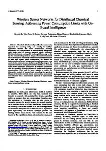
Although the improved systems achieve small false alarm probability, the control packets result in extra power consumption. Fig. 7 shows the total power consumption of 20 sensors under the same scenario as Fig. 6. The total power consumption is calculated by counting the total number of bits transmitted and received by each sensor and using the communication core parameters provided in [1]. We do not consider sensing energy and sensors are assumed to be active all the time. As can be seen in Fig. 7, the improved systems have slightly larger total power consumption than the basic system under the same MAC protocol. Overall the largest increase does not exceed 1.6%. Thus the improved systems achieve much better performance at the expense of minimal energy consumption. Note that here we only consider the energy consumed in monitoring. In reality higher false alarm probability will also increase the alarm traffic volume in the network, thus resulting in higher energy consumption. Also note that the power consumption between different MAC protocols are not comparable because the channel sensing power is not included. Fig. 8 shows the simulation results with various C2 . T = 10 and C1 = 21 are fixed. As can be seen in Fig. 8, when C2 increases, false alarm decreases and the response delay increases. The improved systems have much lower false alarm
T=60sec,C1=121sec
T=60sec,C2=1sec 0.14
0.4 Random Access & Basic System Random Access & Improved System Random Access & The Variation Carrier Sensing & Basic System Carrier Sensing & Improved System Carrier Sensing & The Variation
0.2
0.1
Pr[FA]
Pr[FA]
0.3
Random Access & Basic System Random Access & Improved System Random Access & The Variation Carrier Sensing & Basic System Carrier Sensing & Improved System Carrier Sensing & The Variation
0.12
0.08 0.06 0.04
0.1
0.02 0
0 50
100
150
200
250
300
350
0
20
40
60
80
0
20
40
60
80
100
120
140
160
180
200
100
120
140
160
180
200
400 300
Response Delay
Response Delay
350 300 250 200 150
200 150 100
100 50
50 0 50
C2 (sec) 100
150
200
250
300
350
400
C1 (sec)
Figure 9: The Simulation Results with T = 60, C2 = 1 than the basic system. For the response delay, similar to Fig. 5, the systems with lower false alarm have larger response delays. Furthermore, we can see that in order to reduce false alarm significantly we need to increase C2 significantly for a fixed C1 . However, in practice we should choose to increase C1 rather than increase C2 . This is because by increasing C1 , we can reduce the C1 (i) expiration events and reduce the network traffic, while increasing C2 has no such effect. Increasing C1 has approximately the same effect on the response delay as increasing C2 .
4.3 Light Traffic Load Scenario with T=60 Fig. 9 shows the simulation results with various C1 and T = 60 seconds. Fig. 10 shows the simulation results with various C2 . All results are consistent with previous observations and therefore the discussion is not repeated here.
5.
250
DISCUSSION
In the previous sections we presented a two-phase timer scheme for a sensor network to monitor itself. Under this scheme, the lack of update from a neighboring sensor is taken as a sign of sensor death/fault. We also assumed that connectivity within the network remains static unless attacks or faults occur. If connectivity changes due to disruption in signal propagation, then it becomes more difficult to distinguish a false alarm from a real alarm. If a sensor does not loose communication with all its neighbors then neighbor consultation can still help in this case. As discussed before, if a sensor reappears after a period of silence (beyond the timeout limit), then extra mechanisms are needed to handle alarm reporting and alarm correction. All our simulation results are for isolated death events. In addition we have assumed that sensors are alive all the time. In this section we will discuss our scheme and possible extensions under different attacks and sensor scenarios.
Figure 10: The Simulation Results with T = 60, C1 = 121 B
C
A
Figure 11: Partition Caused by Death
Fig. 11. If sensor A has only one neighbor B and B is dead, no one can monitor A. One possible solution is to use location information. Assuming that the control center knows the locations of all sensors, when the control center receives an alarm regarding B, it checks if this causes any partition by using the location information. If a partition occurs, the control center may assume that the sensors in the partition are all dead. Thus it will attempt to recover all sensors in the partition.
5.2 Correlated Attacks We define by correlated attack the situation where multiple sensors in the same neighborhood are destroyed or disabled simultaneously or at almost the same time. Fig. 12 shows a simple scenario with 7 sensors. Each circle represents a sensor, and a line between circles represents direct communication between sensors. If sensor A is disabled, sensors B, C, and D will detect this event from lack of update from A. Assume C and D are in suspend state because they both received alarm query from B. Thus, only B is responsible for transmitting an alarm for A. Suppose now B is also disabled due to correlated attacks before being able to transmit the alarm. A’s death will not be discovered under the scheme studied in this paper, since both C and D will
C A B
D
`
5.1 Partition Caused by Death Low connectivity of the network may result in security problems under the proposed scheme, e.g., as illustrated in
Figure 12: Correlated Attacks.
T=1sec,C2=1sec 80 Random Access & Improved System Random Access & The Variation Carrier Sensing & Improved System Carrier Sensing & The Variation
75
Alarm Generation Percentage
70
65
60
A
55
50
45
40
35
30
2
2.5
3
3.5
4
4.5
5
5.5
6
6.5
7
C1 (sec)
Figure 13: Alarm Generation Percentage with T=1, C2 = 1
have removed A from their neighbor list by then. This problem can be tackled by considering the concept of suspicious area, which is defined as the neighborhood of B in this case. For example, the control center will eventually know B’s death from alarms transmitted by B’s neighbors, assuming no more correlated attacks occur. The entire suspicious area can then be checked, which includes B and B’s neighbors. As a result A’s death can be discovered. A complete solution is subject to further study. This example highlights the potential robustness problem posed by aggregating alarms (i.e., by putting nodes in the suspend state) in the presence of correlated attacks. The goal of alarm aggregation is to reduce network traffic. There is thus a trade-off between high robustness and low overhead traffic. Intuitively increased network connectivity or node degree can help alleviate this problem since the chances of transmitting multiple alarms are increased as a result of increased number of neighbors. We thus measured the percentage of neighbors generating an alarm in the event of an isolated death under the same scenario as in Fig. 4. The simulation results are shown in Fig. 13. The alarm generation percentage is the ratio between the number of alarms transmitted for a sensor’s death and the total number of neighbors of that dead sensor. As can be seen, all the improved systems have alarm generation percentage greater than 40%. These results are for an average node degree of 6. We also run the simulation for average node degree of 3 and 9. There is no significant difference between these results. Note this result is derived based on an isolated attack model, under which we ensure at least one alarm will be fired (see Proposition 2 in Section 3) even when using alarm aggregation. However, if correlated attacks are a high possibility, we do not recommend the aggregation of alarms, thus removing the suspend state. Further study is needed to see how well/bad alarm aggregation performs in the event of correlated attacks with different levels of connectivity.
5.3 Massive Destruction Fig. 14 illustrates an example of massive destruction, where nodes within the big circle are destroyed, including Sensor A and its neighbors. If this happens simultaneously, the control center will not be informed of A’s death since all the sensors that were monitoring A are now dead. However, the nodes right next to the boundary of the destruction area, i.e., nodes outside of the big circle in this case, are still alive. They will eventually discover the death events of their cor-
Figure 14: Massive Destruction. Nodes with dashed circles are dead sensors. Nodes with solid circles are healthy sensors.
responding neighbors and inform the control center. From these alarms the control center can derive a dead zone (the big circle in Fig. 14), which includes all dead sensors. A’s death will be, therefore, discovered.
5.4 Sensor Sleeping Mode Sensors are highly energy constrained devices, and a very effective approach to conserve sensor energy is to put sensors in the sleeping mode periodically. Many approaches proposed use a centralized schedule protocol, e.g. TDMA, to perform sleep scheduling. Although our improved mechanism is not designed for such collision-free protocols, it can potentially be modified to function in conjunction with the sensor sleeping mode. A straightforward approach is to put sensors in the sleeping mode randomly. However, by doing so a sensor may lose packets from neighbors while it is asleep, which then increases the false alarm probability. Increased timer value can be used to reduce false alarm at the expense of larger response delay. In [9] a method is introduced to synchronize sensors’ sleeping schedule. Under this approach, sensors broadcast SYNC packets to coordinate its sleeping schedule with its neighbors. As a result, sensors in the same neighborhood wake up at almost the same time and sleep at almost the same time. Sensors in the same neighborhood contend with neighbors for channel access during the wake-up time (listen time). In our scheme studied in this paper, the control packets (Pex , Paq , and Par ) can all be regarded as the SYNC packets used to coordinate sensor sleep schedule. The stability of coordination as well as the resulting performance need to be further studied.
5.5 Response Delay The improved system may have longer response delay than the basic system. Fig. 15 shows such a scenario. In the improved system, if sensor A fails to receive the last Pex from neighbor i and i is dead right after this failure, A sends Paq to neighbors upon C1 (i) expiration in the improved system. Its neighbor B successfully receiving the last Pex from i responds with a Par including a C1 (i) reset value. Thus, A resets its expired C1 (i) when it receives Par . An alarm for i will be fired after this new C1 (i) and C2 (i) expire. However, in the basic system sensor A fires an alarm upon the expiration of the original C(i), which in this scenario occurs earlier than in the improved system. Note that although the response delay in the improved system is sometimes longer
7. REFERENCES
Sensor i is dead Send Pex(i)
Send Pex(i)
(1)Basic: Neighbor A
Alarm Response Delay
R
L C=C1+C2
(2)Improved:
Alarm Response Delay
Neighbor A
R
L Remaining C1
C1
C2
query
Alarm
Neighbor B
R
R C1
C2
Figure 15: Event Schedule of A Potential Problem. “R” means Pex is received. “L” means Pex is lost. than the basic system, the response delay is bounded by C1 + C2 . Also note that the above scenario can occur in opposite direction as well, i.e., alarm is fired earlier in the improved system.
5.6 Update Inter-Arrival Time In our simulation, the existence/update packet inter-arrival time is exponential distributed with mean T in order to obtain a large variance to randomize transmissions. As shown in the simulation results, when T is large, the variance of the inter-arrival times is also large. As a result a large C1 is needed to achieve small false alarm probability. An alternative is to use a fixed inter-arrival time T along with proper randomization via a random delay before transmission. By doing this, we can eliminate the false alarm caused by the large variance of the update inter-arrival time when the network traffic load is light (T is large).
6.
CONCLUSION
In this paper, we proposed and examined a novel distributed monitoring mechanism for a wireless sensor network used for surveillance. This mechanism can monitor sensor health events and transmit alarms back to the control center. We show via simulation that the proposed two-phase mechanism (both the original and the variation) achieves much lower probability of false alarm than the basic system with only one timer. Equivalently for a given level of false alarm probability, the improved systems can achieve much lower response delays than the basic system. These are achieved with minimal increase in energy consumption. We also show that carrier sensing performs better than random access and their performances converge when we increase the average update period T . Increasing timer values results in lower false alarm and larger response delays. There are many interesting problems which need to be further studied within the context of the proposed mechanism, including those discussed in Section 5. Different patterns of attacks and their implication on the effectiveness of the proposed scheme needs to be studied. Necessary modifications to our current scheme will also be studied in order for it to efficiently operate in conjunction with sensor sleeping mode.
[1] M. Bhardwaj and A. P. Chandrakasan. Bounding the lifetime of sensor networks via optimal role assignments. In IEEE InfoCom, 2002. [2] D. Ganesan, R. Govinda, S. Shenker, and D. Estrin. Highly resilient, energy efficient multipath routing in wireless sensor networks. Mobile Computing and Communications Review (MC2R), 1(2), 2002. [3] J. Heidemann, F. Silva, C. Intanagonwiwat, R. Govindan, D. Estrin, and D. Ganesan. Building efficient wireless sensor networks with low-level naming. In Proceedings of the Symposium on Operating Systems Principles, pages 146–159, October 2001. [4] W. Heinzelman, A. Chandrakasa, and H. Balakrishnan. Energy-efficient communication protocols for wireless microsensor networks. In Proceedings of Hawaiian International Conference on Systems Science, January 2000. [5] C. Intanagonwiwat, D. Estrin, and R. Gonvindan. Impact of network density on data aggregation in wireless sensor networks. In International Conference on Distributed Computing Systems (ICDCS-22), November 2001. [6] J. Kulik, W. R. Heinzelman, and H. Balakrishnan. Negotiation-based protocols for disseminating information in wireless sensor networks. ACM Wireless Networks, 8, 2002. [7] L. Subramanian and R. H.Katz. An architecture for building self-configurable systems. In IEEE/ACM Workshop on Mobile Ad Hoc Networking and Computing (MobiHOC 2000), 2000. [8] A. Woo and D. E. Culler. A transmission control schemes for media access in sensor networks. In ACM/IEEE International Conference on Mobile Computing and Networking (MOBICOM), 2001. [9] W. Ye, J. Heidemann, and D. Estrin. An energy-efficient mac protocol for wireless sensor networks. In IEEE InfoCom, 2002. [10] Y. J. Zhao, R. Govindan, and D. Estrin. Residual energy scan for monitoring sensor networks. In IEEE Wireless Communications and Networking Conference (WCNC’02), March 2002.