A Distributed System for Storing and Processing Data from Earth-observing Satellites: System Design and Performance Evaluation of the Visualisation Tool Marek Szuba∗‡ , Parinaz Ameri∗§ Udo Grabowski†¶ , Jörg Meyer∗k and Achim Streit∗
∗∗
arXiv:1511.07693v2 [cs.DC] 10 Feb 2016
∗ Steinbuch
Centre for Computing (SCC) of Meteorology and Climate Research (IMK) Karlsruhe Institute of Technology Hermann-von-Helmholtz-Platz 1 76344 Eggenstein-Leopoldshafen, Germany E-mail: ‡
[email protected] §
[email protected] ¶
[email protected] k
[email protected] ∗∗
[email protected] † Institute
Abstract—We present a distributed system for storage, processing, three-dimensional visualisation and basic analysis of data from Earth-observing satellites. The database and the server have been designed for high performance and scalability, whereas the client is highly portable thanks to having been designed as a HTML5- and WebGL-based Web application. The system is based on the so-called MEAN stack, a modern replacement for LAMP which has steadily been gaining traction among high-performance Web applications. We demonstrate the performance of the system from the perspective of an user operating the client. Index Terms—Distributed processing, geospatialdata analysis, Web application, MEAN stack, MongoDB, AngularJS, Express, Node.js, WebGL.
I. Introduction The processing of satellite observations of Earth is highly data-intensive. Many satellites produce highresolution images of the Earth. Many observational missions were or have been in operation for decades. In some cases the raw input itself may not be so large but processed, analysis-ready data is. Either way, Earth-observing satellites can now be considered a fully fledged source of Big Data. One such source has been the Michelson Interferometer for Passive Atmospheric Sounding on the ESA Envisat satellite, a Fourier-transform spectrometer. MIPAS operated between 2002 and 2012, and measured geotemporal distribution in the atmosphere of more than 30 trace gasses relevant to atmospheric chemistry and climatechange research. Data from MIPAS is stored in several different data archives, including the Large-Scale Data Facility (LSDF) [1] at the Karlsruhe Institute of Technology (KIT). As of August 2015, the complete MIPAS archive at LSDF requires around 30 TB for the storage of calibrated measurement data released by the ESA (“level-1B data”)
and around 64 TB for processed (“level-2”) data produced from the former at KIT. Both parts will continue to grow in the near future. MIPAS data at LSDF consists primarily of compressed text and PostScript files as well as some classic-format NetCDF files. Analysis of this data involves several difficulties: there are many different sources of input, data is separate from at least parts of its metadata, repeated parsing of text can be time consuming, compressed files must be wholly decompressed on the fly, data inside classic NetCDF files is not indexed. In short, working with filesystem MIPAS data can be quite slow. The situation becomes even more complicated when a comparative analysis of data from different experiments is desired, for example from MIPAS and the Microwave Limb Sounder (MLS) on the NASA Aura satellite. With different experiments structuring their data in different ways, the conventional analysis approach requires developing and running several different pipelines even though the analysis algorithm itself remains the same. Moreover, even when multiple experiments cover the same locations and time span, exact coordinates and time stamps of their respective data points are only similar, not the same — requiring another round of data processing in order to match them. In light of the above we have proposed and implemented an alternative, distributed and scalable solution, which takes advantage of Big Data tools and methods in order to improve performance of working with MIPAS and similar data. In the following sections we shall describe our system and present an analysis of chosen aspects of its performance. The structure of the following parts of the paper is as follows. In Section II we describe the architecture of our system, discussing each of its tiers, whereas Section III
presents the evaluation of the system’s performance from the point of view of the user of the client application. Section IV mentions several related tools and systems. Finally, in Section V we present our conclusions and the the outlook for the project. II. System Architecture The goals we set while designing our system were as follows: • it should scale well as the amount of data stored in it grows; • it should facilitate the use of data from multiple sources; • the basic user interface should be easy to access and use. We have chosen the standard multi-tier design model consisting of the database, the server and the client, common among Big Data applications. It allows for independent growth of each of the tiers as needed as well as performing computation-intensive processing on more powerful systems than what the client might have at their disposal or data-size reduction closer to the database. Our system is based on the NoSQL database MongoDB, the server-side runtime platform Node.js, the Web-application framework Express and the JavaScript MVC framework AngularJS, known together as the MEAN stack and offering a number of advantages over more established stacks such as LAMP to both users and developers [2]. The eventual architecture of our system is shown in Figure 1. We implement the data browser as a Web application to ensure portability and make it easier for users to keep it up to date. Furthermore, by making our client a single-page application we essentially add another degree of scalability to the system. A. The Database Our MongoDB system presently runs on a single, dedicated server and contains data from MIPAS, MLS and a number of other, smaller experiments, each with its own database. Data for each geotemporal location constitutes a single document. We have developed several tools which communicate directly with the database server using appropriate MongoDB drivers, for example a Python tool which can be used to perform general matching of data from two different sources (e.g. MIPAS and MLS); it is capable of multithreaded operation and has already been used to demonstrate superior performance of MongoDB comparing to a SQL database system [3]. B. Server-side Processing and REST API Since our main client is a Web application, making our instance of MongoDB accessible from the Internet is impractical because it would require adding a MongoDB driver to the user’s browser. Using an intermediate server means a server-installed driver can be used, whereas
communication with clients occurs using HTTP. Such a server can also perform pre-processing before passing the data between the client and the database. The underlying platform of our server is Node.js and the HTTP Representational State Transfer (REST) client API is based on Express. Data is transferred in JSON format. Our server is based on an in-house distributed solution called Node Scala [4]. The reason for this is that while undoubtedly optimised for performance, Node.js applications are by design restricted to a single thread. Distributed systems featuring multiple instances of the same application accessed through a common interface such as the same HTTP server, can be constructed using the standard Node.js module Cluster (on a single host) or third-party solutions built on top of it such as StrongLoop Process Manager (which can support multiple hosts), however neither of these solutions allow for parallel processing. Conversely, Node Scala does allow parallel execution of tasks with intelligent distribution of chunks among backend servers (i.e. workers) and supports the spawning and monitoring of back-end servers on both the same and multiple hosts. Please see [4] for more information about Node Scala and its performance. In its current configuration our Node Scala instance runs on a single, dedicated server. It uses a single front-end server offering the MIPAS REST API over HTTPS and two back-end servers which handle communication with the database server as well as data processing. Following the rule of least privilege, back-end servers are only allowed to read from the database. C. The Client Our new client application, KAGLVis, is a data browser which displays selected observables as 3D points at correct coordinates on a virtual globe. At present it can display orbital paths of Envisat as well as cloud altitude measured by MIPAS, in the latter case allowing the user to specify criteria defining clouds. The data is fetched from the server in the background, depending on the user’s preferences either set by set or simultaneously for the whole selected range. The view, which can be either a sphere, a plane or that of poles and which allows for selection of a number of different Earth images as background, can be freely rotated and zoomed. The colour map in the legend is drawn dynamically on a HTML5 canvas element and synchronised with the contents of the 3D view. It is worth emphasising at this point that KAGLVis is not meant as a replacement for the plethora of standard data-processing tools used in geosciences. Instead, KAGLVis aims to provide basic visualisation and analysis capabilities as easily as possible. The internal logic of KAGLVis has been implemented using AngularJS, with each component of the view assigned its own controller. All communication between components occurs explicitly through messages sent via a dedicated internal service; no communication through
REST over HTTP(S)
Back-end server
Shard
Front-end server Back-end server
Shard
...
Query router
...
...
User
Load balancer User
...
Front-end server Shard
MongoDB
User
Back-end server
Node Scala
KAGLVis
Figure 1. Architecture of our system. For clarity, the diagram omits internal management components of Node Scala (the controllers and the scheduler) as well as the Web server used to serve KAGLVis files to users.
e.g. global variables is allowed. Another service provides access to configuration of the application. Finally, the third service provides an interface to the data source — which by default is our REST server but can if need be, for testing for instance, switched to a local JSON file. The heart of KAGLVis, the 3D display, is based on WebGL Globe — a lightweight JavaScript virtual globe created by Google Data Arts Laboratory which can display longitude-latitude data as spikes. As the name suggests, Globe uses WebGL to leverage local GPU power for 3D rendering. Our version of Globe has been customised to support other views than the original sphere as well as selection of the background texture, reduce memory consumption at a cost of disabling certain visual effects, and most importantly to allow caching of previously displayed data sets should the user want to return to them at some point. Testing has shown KAGLVis is indeed highly portable — it has been confirmed to run without errors on many Web browsers and operating systems, including on mobile devices. We use a minimal Express-based Web server to serve KAGLVis to users. The server is hosted on the same system as the REST server because, as a single-page application, KAGLVis adds only minimal load to the server hosting it. III. Evaluation We have measured performance and resource use of KAGLVis under realistic operating conditions. There are
Figure 2. A screenshot of KAGLVis showing cloud altitude measured by MIPAS against flat Earth view.
three reasons for focusing on the client: it is the component through which our system is experienced by most users, Web browsers are not as strongly optimised for performance as MongoDB and Node.js, and some benchmarks of back-end components of our system have already been published (see e.g. [3], [4]). Our tests were executed on a PC with an Intel Core i54300U CPU with HD 4400 graphics, 12 GB of DDR3/1600 RAM, and a LCD screen at its native resolution of
displayTime / nPoints [us]
nPoints
1000
800
600
800
600
400
400
200
200 0
0
5
10
15
5
10
15
20
Day #
20
Day # Figure 3. Number of data points for each day of Envisat MIPAS data used in subsequent tests. Horizontal axis: index of the day in the complete test sample. Vertical axis: number of data points the day contains.
1920x1200 pixels at 60 Hz. The system ran an up-to-date 64-bit installation of Gentoo Linux, including X.org server 1.16.4 and the video driver xf86-video-intel 2.99.917. All tests were run in the Chromium 44.0.2403.89 Web browser using one of its built-in developer tools, Timeline [5]. The client connected to our production REST server (the technical details of which can be found in [4]), using IPv4 over a Gigabit Ethernet connection. We benchmarked the visualisation of cloud altitude measured by MIPAS. This application relies on user input and thus requires some client-side processing of data. For each test and iteration we launched Chromium fresh and recorded Timeline events from KAGLVis for up to 20 days’ worth of data, a number high above typical usage patterns — already at 5 days parts of the map become too crowded to be read comfortably. The number of usable MIPAS data points per day varies. Figure 3 shows the number of points for each day displayed during testing. In order to account for differences in dataset size we, where appropriate, normalised results of our measurements to the number of points in each day. A. Time to Display To measure how responsive KAGLVis it is to input, we first measured how long takes to display a new data set on the screen — i.e. convert JSON input to a 3D mesh, add that mesh to the WebGL scene and update the view to reflect the changes — after it has been requested by the user. Subsequent days are combined with previously displayed content instead of replacing it so that we can
Figure 4. Time required to add a day’s worth data to the view. Horizontal axis: index of the day in the complete test sample. Vertical axis: time required to display the day divided by the number of data points it contains.
watch for possible scalability problems. We explicitly excluded data-transfer time from the benchmark because network transfers in KAGLVis occur asynchronously in the background, not affecting interface responsiveness. As Figure 4 shows, for most data sets it consistently takes around 300 µs per point, or 0.3 s whole, to display. The exception, day 4, seems to be caused by the WebGL implementation in Chromium — Timeline shows that while the time required to add this day to the scene is consistent with that for other data sets of similar size, the subsequent animation-frame update not only takes considerably longer than for all other data sets but is in fact split into three separate steps. For days low-point days 8–11 the behaviour is different — around 600 µs per data point (amounting to 1–2 s per whole data set), with considerable fluctuations between iterations. Given the detailed structure of Timeline events for these and other days appears to be very similar, it is believed that for data sets so small the measured time becomes dominated by the processing overhead. Finally, for day 1 the time of almost 780 µs per point is even slightly higher, while fluctuating less, than for other small data sets As the Timeline structure of the animation-frame update step here is very different from that for subsequent data sets, we concluded what we see here is both processing overhead and effects of WebGL initialisation. B. Memory Consumption Secondly, we measured the growth of the JavaScript heap of KAGLVis as we load more and more data sets
Frame rate [FPS]
heapSizeIncrease / nPoints [kB]
20
Intel
80
Radeon
70 60 50 40
15
30 20 10
0
5
10
15
20
Day # Figure 5. Evolution of memory consumption as more and more data is added to the view. Horizontal axis: index of the day in the complete test sample. Vertical axis: difference in JavaScript heap size after another day’s worth of data has been displayed and before it has been loaded into the view, divided by the number of data points in each day.
into it. The results can be found in Figure 5. A consistent increase of around 12 kB per data point can be observed from day 3 onward — suggesting the test system could cache hundreds of days’ worth of data before running out of physical RAM. Above-average value of 22 kB per point measured for day 1 is consistent with our earlier hypothesis of the loading of the first data set triggering initialisation of internal data structures. It is presently not fully understood why an above-average value can also be observed for day 2. C. Frame Rate Finally, we used the FPS counter built into Chromium to measure the frame rate of KAGLVis window as a function of the number of simultaneously shown data sets. As integrated graphics chipsets are generally not performance-oriented, we repeated this test on an otherwise similar PC with an AMD Radeon HD 4770 PCIe graphics card. Apart from the graphics driver (Mesa-10.3.7 with Gallium3D driver “r600” + X.org driver xf86-videoati 7.5.0) the software on both systems was identical. What makes this comparison particularly interesting is that we are comparing a relatively recent Intel graphics chipset with a device which while originally marketed as mid-range is now quite old — the two were released in late 2013 and early 2009, respectively. Measurements were repeated five times for each set-up and their results can be found in Figure 6. The frame rate drops dramatically as more data is added to the view. With all points visible it is just under
0
0
5000
10000
15000
Data points loaded Figure 6. Frame rate as a function of the number of data points simultaneously displayed on screen. Black: results from our standard test system. Red: results from a machine with AMD Radeon graphics.
12 FPS, resulting in noticeable jerkiness of animation during rotation or zooming. That said, frame rates in the typical use range of under 5,000 points appear to be sufficient. Despite its age the Radeon card outperforms the Intel chipset: around 34 FPS for all points and above 50 FPS in the typical use range. A number of peculiarities can be observed in the results. To begin with, the frame-rate drop does not scale linearly with the number of points. Instead, it becomes smaller and smaller as more data is added to the view. It is furthermore interesting that such low frame rates are seen for a fairly uncomplicated and essentially static scene, especially given the very same system consistently outputs more than 30 FPS running a highly dynamic and complex WebGL water simulation. All in all it would seem that the observed behaviour is driven primarily by the properties of the WebGL engine provided by Chromium, although given the behaviour of the aforementioned water test optimisation of WebGL use in Globe might improve its 3D performance as well. IV. Related Work Given both the number of different components a system capable of comprehensive handling of geospatial data must contain and how widespread the handling of such data has become in modern science, it is not surprising the amount of work put into this topic has been considerable. Here are some examples. On the database side one should definitely mention PostGIS [6], a spatial database extension for the Postgr-
eSQL relational database system which is supported by a wide range of GIS applications. However, as a RDBMS it is not in direct competition with NoSQL-based systems like ours. Even if only Node.js-based solutions are considered, the number of alternatives for server-side code is considerable. Then again, each of them has certain shortcomings — which ultimately led us to develop Node Scala. Please see [4] for details on this matter. Likewise there are many solutions for visualisation of geospatial data and each of them has disadvantages from our perspective. For example, the popular and open NASA World Wind [7] is presently only suitable for standalone applications and would introduce another programming language (Java) into the stack, while at the same time a lot of its features and detail are simply unnecessary while dealing with high-altitude data from satellites. Another alternative, Google Earth Engine [8], is not unlike our own system in that it is an all-in-one solution handling both storage, data-management and analysis through a highly distributed Web application — but does not presently give most of its users the possibility to develop own processing algorithms, is a closed platform tied to Google computing infrastructure, and most importantly can only be used to process data made available by Google. Another example is the highly popular UltraScale Visualisation Climate Data Analysis Tools (UV-CDAT) framework [9]. UV-CDAT and our system complement rather than compete with each other: the latter attempts first and foremost to provide high-performance access to data, the latter focuses on data analysis. Finally, the German Satellite Data Archive (D-SDA) of the Earth Observation Center at the German Aerospace Center (DLR) [10] at a glance seems to serve the same purpose as our system yet is backed by considerably more resources. There are, however, differences: it is tied to DLR infrastructure, keeps both data and metadata as files in storage rather than in a database, and most importantly follows considerably different philosophy — its primary goal is to achieve long-term data preservation over more than 20 years with nearly exponentially growing data capacity, whereas our archive has been designed primarily to provide high-performance access to a fixed chunk of data. One could therefore imagine the two systems as complementary — ours for rapid application-specific processing, D-SDA for long-term storage. V. Conclusions and Future Work We have demonstrated a distributed, high-performance and scalable system based on the so-called MEAN stack, which is used to store, process and visualise data from the ESA Envisat Earth-observing satellite. Benchmarks of the system as seen from the end-user’s perspective demonstrating good performance even beyond the typical
use range and on a system without a discrete graphics device. In the near future we will continue importing further MIPAS data into MongoDB as well as prepare for the migration of the production database to a sharded cluster. The REST server shall be extended accordingly, with new use cases and more back-end servers. Finally, we would like to improve KAGLVis user experience on mobile devices. Acknowledgements This work is funded by the project “Large-Scale Data Management and Analysis” [11], funded by the German Helmholtz Association. References [1] A. Garcia, S. Bourov, A. Hammad, J. van Wezel, B. Neumair, A. Streit, V. Hartmann, T. Jejkal, P. Neuberger, and R. Stotzka, “The Large Scale Data Facility: Data Intensive Computing for Scientific Experiments,” in Parallel and Distributed Processing Workshops and PhD Forum (IPDPSW), 2011 IEEE International Symposium on, May 2011, pp. 1467–1474. [2] V. Karpov. The MEAN Stack: MongoDB, ExpressJS, AngularJS and Node.js. (last visited: 2015-11-06). [Online]. Available: http://blog.mongodb.org/post/49262866911 [3] P. Ameri, U. Grabowski, J. Meyer, and A. Streit, “On the Application and Performance of MongoDB for Climate Satellite Data,” in Proceedings of the 13th IEEE International Conference on Trust, Security and Privacy in Computing and Communications, 2014, pp. 652–659. [4] A. Maatouki, M. Szuba, J. Meyer, and A. Streit, “A horizontally-scalable multiprocessing platform based on Node.js,” in Proceedings of the 13th IEEE International Symposium on Parallel and Distributed Processing with Applications (to be published), 2015, arXiv:1507.02798 [cs.DC]. [5] Performance profiling with the Timeline. (last visited: 201511-06). [Online]. Available: https://developer.chrome.com/ devtools/docs/timeline [6] C. Strobl, “PostGIS,” in Encyclopedia of GIS., S. Shekhar and H. Xiong, Eds. Springer, 2008, pp. 891–898. [Online]. Available: http://dx.doi.org/10.1007/978-0-387-35973-1_1012 [7] P. Hogan, “NASA World Wind: Infrastructure for Spatial Data,” in Proceedings of the 2nd International Conference on Computing for Geospatial Research & Applications, ser. COM.Geo ’11. New York, NY, USA: ACM, 2011, pp. 2:1– 2:1. [Online]. Available: http://doi.acm.org/10.1145/1999320. 1999322 [8] N. Gorelick, “Google Earth Engine,” in EGU General Assembly Conference Abstracts, ser. EGU General Assembly Conference Abstracts, vol. 15, Apr. 2013, p. 11997. [9] D. N. Williams, T. Bremer, C. Doutriaux, J. Patchett, S. Williams, G. Shipman, R. Miller, D. R. Pugmire, B. Smith, C. Steed, E. W. Bethel, H. Childs, H. Krishnan, P. Prabhat, M. Wehner, C. T. Silva, E. Santos, D. Koop, T. Ellqvist, J. Poco, B. Geveci, A. Chaudhary, A. Bauer, A. Pletzer, D. Kindig, G. L. Potter, and T. P. Maxwell, “Ultrascale Visualization of Climate Data,” Computer, vol. 46, no. 9, pp. 68–76, 2013. [10] C. Reck, E. Mikusch, S. Kiemle, K. Molch, and W. Wildegger, “Behind the Scenes at the DLR National Satellite Data Archive, a Brief History and Outlook of Long Term Data Preservation,” in Proceedings, PV 2011: Ensuring Long-Term Data Preservation, and Adding Value to Scientific and Technical Data, Toulouse, France, Nov. 2011, http://elib.dlr.de/74103/. [11] C. Jung, M. Gasthuber, A. Giesler, M. Hardt, J. Meyer, F. Rigoll, K. Schwarz, R. Stotzka, and A. Streit, “Optimization of data life cycles,” J. Phys. Conf. Ser., vol. 513, p. 032047, 2014.