A DRC Based Algorithm for Extraction of Critical ... - Semantic Scholar

IE E E Tr a n s a c ti o n s o n C o m p u te r - A i d e d D e s i g n , v o l . 1 8 , n o . 2 , Fe b . 1 9 9 9

A DRC Based Algorithm for Extraction of Critical Areas for Opens in Large VLSI Circuits Witold A. Pleskacz, Charles H. Ouyang and Wojciech Maly Department of Electrical and Computer Engineering Carnegie Mellon University 5000 Forbes Ave., Pittsburgh, PA 15213

Abstract This paper describes an algorithm for the extraction of the critical area for opens. The presented algorithm allows for the analysis of industrial size ICs with non-Manhattan geometry. Illustrative examples of the proposed algorithm, implemented by using design rule checker operations, are presented. It is shown that the extraction of the critical area for realistic size VLSI circuits designs can be done in an acceptable time.

1. Introduction1 Yield loss is the result of many complex physical phenomena disturbing IC manufacturing Ð some of them occurring infrequently and some of them being inherent artifacts of the applied technology. Phenomena causing opens in VLSI IC interconnects are not believed to be among the top few yield detractors. There are, however, phases of process development and types of technologies in which opens cannot be ignored, and in which prediction of yield loss due to opens must be performed. The first yield model targeting opens and applying the concept of the critical area was published a long time ago [1]. Since then a few approaches attempting to include opens in the yield prediction have been published [2, 3, 4, 5, 6, 7, 8]. The vast majority of the published approaches, however, have been focused on the accuracy of estimation, which have resulted in algorithms which are too complex to handle modern multi-million transistor devices. As a result, even if the basic idea proposed in [1] is simple and still valid, there is no efficient yield estimation methodology until now which can handle opens in large modern VLSI ICs. Spot defect based yield loss prediction involves critical area estimation and extraction of the characteristics of the spot defects causing yield loss. This paper deals with critical area estimation only. The methodology for extraction of defect characteristic [11, 12] and yield modeling using 1

Portions of this paper have been published in [16, 17].

Ð1Ð


critical area [2, 3, 4, 5, 6, 7, 8, 9, 10] has been proposed and discussed in detail. This paper discusses an algorithm for extracting the critical area for defects causing opens. The organization of the paper is as follows. First a discussion of the concept of critical area for opens is presented. The focus of the discussion is on metal interconnection with special emphasis on contacts and vias. Next a set of generic layout manipulation procedures, which are used in the critical area extraction algorithm, is listed. Then the critical area extraction algorithm is introduced and its complexity is discussed in detail. Finally, examples are presented to illustrate the proposed algorithm and to assess its computational efficiency.

2. Critical area for spot defects causing opens 2.1. Spot defects Spot defects in an IC are caused by contaminants introduced by the manufacturing process. They can be seen as severe but local, often three-dimensional (3-D), deformations of the IC structure. Under certain situations, defects may cause breaks or excessive resistance in a connection resulting in an open circuit. This paper deals with spot defects causing opens in conducting IC layers. Spot defects can occur in a single layer or can affect more than one IC layer. In this paper spot defects are modeled as disks of missing conducting material in the conducting layer or disks of extra insulating material in the insulating layer. Important characteristics of spot defects are: size (expressed by the radius R) and frequency of occurrence (density). This paper is restricted to defects affecting single layers. Observe, however, that a single layer defect occurring in the oxide layer may affect connectivity between two conducting layers separated by the oxide (see Fig. 1).

AAAAAAAAAAAAA AAAAAAA AAAAAAAAAAAAA AAAAAA AAAAAAAAAAAAA AAAAAAA AAAAAAAAAAAAA AAAAAAAAAAAAA AAAAAAA AAAAAA AAAAAAA AAAAAA AAAAAAAAAAAAA AAAAAAA AAAAAA AAAAAA AAAAAAAAAAAAA AAAAAAA AAAAAA AAAAAA AAAAAA AAAAAAAAAAAAA AAAAAAA AAAAAA AAAAAA AAA AAAAAA AAAAA AAAAAAA AAAAA AAAAAAAAAAAAAA AAAAAAAAAAAAAAAAAAA AAAAAAA AAAAAAAAAAAAA AAAAAA AAAAAA AAAAAA AAAAAAAAAAAAA AAAAAA AAAAAA AAAAAAAA AAA AAAAAA AAAAA AAAAAAAAAAAAAA AAAAAAA AAAAA AAAAAA AAAAA AAAAAAAAAAAAAA AAAAAAA AAAAAA AAAAAA AAAAA AAAAAAAAAAAAAAAAAAAAAAAAAAAA SiO 2

Al

SiO 2

SiO 2

SiO 2

SiO 2

Al

SiO 2

SiO 2

Si

SiO 2

Si

(a)

defect

(b)

Figure 1. Well contact: (a) functional contact; (b) contact deformed by defect. 2.2. Definition of the critical area for an open There are two attributes of a ÒgoodÓ electrical connection in an IC chip. The first is physical continuity of the conducting paths. The second is good electrical contact between conducting

Ð2Ð


layers. (Good electrical contacts play an especially important role in sub-micron technologies.) This section discusses the concept of critical area Ð a measure of IC layout sensitivity to spot defects Ð by considering both interconnect continuity and inter-layer contacts. According to the generic definition in [1] the critical area for opens are regions enclosing all locations of spot defect centers which result in interconnect opens. A typical interconnect is a chain of conducting segments on different layers (see Fig. 2) and contact plugs formed to provide connections between these segments. Hence, to assess the probability of an open one needs to compute the critical area for each segment of interconnect and for the contacts in the analyzed layout [7, 8]. Below both problems are discussed in detail. Interconnect segment

A AAA AAAAAAAAA A AAA AAAAAAAAAAA AAAAAAA AAAAA AAAA AAA AAAAA AAAA AAAAA AAAAAAAAAA AAA A AAAAAAAAA AAA AAAAAAAAA AAAAAAAAAAA AAAAAAA AAAAA AAAA AAAAAAAAAA AAA AAA AAAAA AAAAAA AAAA AAA AAAAAAAAA A AAA AAAAAAAAAAA AAAAAAA AAAAA AAAA AAA AAAAA AAAA AAAAA AAAAAAAAA AAA AAAAAAAAA AAAAAAAAAA AA AAA AAAAAA AAAA A AAAAAAAAA AAAAAAAAA AAAA AAAAA AAA AAA AAAAAAAAA AAAAAAAAAAA AAAAAAAAAA AA AAA AAA AAAA AAAAAA AAAA AAAA AAA AAAAAAAAAAAAAAAAAAAAAAAAAAAAAAAAA AAAAAAAAA A AAAAAAAAA AAAA AAAAA AAA AAA AAAAAAAAAAA AAA AAA AAAA AAAA AAAA AAA A AAAAAAAAAAAAAAAAAAAAAAAAAAAAAAAAA AAAAAAAAA A AAAAAAAAAAAAAAAAAAA AAAA AAAAAA AAAAAAAA AAAA AA AAA AA AA AAA AA Al

Al

SiO 2

SiO 2

Al

SiO 2

Al

Al

SiO 2

SiO 2

SiO 2

Ohmic junctions

Tungsten plug

First metal layer

Second metal layer

Figure 2. Interconnect chain.

Critical area for conducting segment of an interconnect Any segment of a VLSI interconnect can be viewed as a conducting path terminated with two or more contacting regions (see Fig. 3). Contacting regions are areas of the physical ohmic junction between different conducting layers. It is important to underline that contacting regions belong to the conducting layers (e.g. Metal 1, Metal 2, Poly, etc.), but do not belong to Contact or Via layers. Electrical terminal of conducting path

AAA AAA AAA

Conducting path

Contacting region

AAA AAA AAA

Figure 3. Typical segment of a VLSI interconnect.

Ð3Ð


A conducting path is broken (open) if a spot defect spans two opposite edges of the conducting path (see Fig. 4a and 4b). Consequently, the critical area for a conducting path can be determined by constructing a set of points located within a distance equal to the radius R of the defect from both edges of this path. Observe that a such set can be obtained by appropriate shifts of the edges of the conducting path (see Fig. 4c and Fig. 5 [7, 8]). One can use, for this purpose, contour manipulation procedures which are discussed later in this paper in detail. Observe also that the assumption about the circular shape of a defect results in a complex shape of critical area boundaries. (See the ends of the critical area regions in Fig. 4c.) Such complexity is neither desired nor necessary. Simply by approximating the shape of the defect by the bounding box of the disk (see Fig. 4d), one can obtain a critical area without arcs (which would difficult to deal with). For this reason it is assumed in this paper that defects are adequately represented by squares with a side 2R long.

(a)

Conducting path

R

Spot defect ( missing material in conducting layer )

(b)

Catastrophic defects

A AAAAAAAAAAA AA AAAAAAAAAAA

(c)

R

R

Critical area

(d)

R

R

R

Critical area

Figure 4. Concept of the critical area for opens: (a) equipotential conducting path; (b) example of different spot defect locations; (c) critical area for opens for the single conducting path; (d) critical area using square defects.

Ð4Ð


A critical area for a contacting region is also easy to construct. An open occurs there when a spot defect of radius R entirely covers the contacting area. For simplicity it is assumed in this paper that such an area can be approximated by a rectangle formed by contact edges shifted by radius R (see Fig. 6). Of course, the total critical area for an open in a segment of an interconnect is a union of the critical areas computed for the conducting path and contacting regions (see Fig. 7).

A AAAA AAAAA AA AAAAAAAAA AA AAA AA AAA R

R

R

R

Critical area for conducting path

Figure 5. Critical area for the conducting path of the segment of Fig. 3.

AA A AAA

AA AAA AAA AA A

R

R

Critical area for electrical terminals

Figure 6. Critical area for the contacting regions.

AA AAAAAAAAA AA AA AAAAAAAAA AA Total critical area

Figure 7. Total critical area for an open caused by a defect of radius R. Opens in contact and via layers To simplify the discussion it is assumed in this paper that any interference with the contact or via process causes an unacceptable increase in contact resistance. (Fig. 8 illustrates one possible mechanism of contact or via degradation due to a spot defect.) Therefore, the failure criterion is: ¥ A defect will cause a failure if it overlaps any portion of the contact or via. In such a case the critical area for opens is defined as the region which contains centers of all defects of a given radius R touching any part of a contact cut or via region (see Fig. 9).

Ð5Ð


Metal 2

(a)

AAAAAAA AAAAAAAAAAA AAAAAAAA AAAA AAAA AAAAAAA A AAAAAAAAAAAA AAAAAAA Metal 1

(b)

AA AA AAAA AA AA AA AAAA A AA AA AAAA AA AA AAAA AA AA AAAA AA AA AAAAAA A AAAA AA AA A AAAAAA A AA A Al

W

SiO2

Metal 1

Unacceptable deformation of contact area

Defect

Contact cut

Al

Spot defect

Figure 8. Mechanism of contact or via degradation due to spot defects: (a) layout; (b) cross section of simplified via structure with defect; Al Ð Aluminum, W Ð Tungsten.

AAAAAA AAAAAA AAAAAA AAAAAA AAAAAA

Critical area

R

Contact cut

R

Spot defect Figure 9. Concept of the critical area for opens in contacts and vias. Finally note that the approach presented so far is valid for a single contact or via. In a typical design, however, there are many cases in which multiple contacts and contact banks are used to connect two conductive segments in different layers. Contact banks are designed with a desired resistance specification in mind. A single defect can cause a contact bank to fail only if it overlaps with multiple contacts and causes enough contacts to fail such that the resistance specification of the entire contact bank can no longer be met. Therefore, the failure criterion is:

Ð6Ð


¥ A defect will cause the contact bank to fail if it overlaps n or more contact or via cuts, where n is the number of redundant contacts built into the connection. Consequently, the critical area of a contact bank, for a defect radius R, can be determined by constructing regions which contain all points located less than a distance R away from n or more contacts. Consider the example in Fig. 10. The set of points up to R units away from each individual contact can be found by shifting the edges of each contact by R (see Fig. 10b). Notice that the sets of points created for each contact intersect. The number of sets to which an individual point belongs is equal to the number of contacts which are no more than R units away from this point (see Fig. 10c). So, the critical area of the contact bank can be found by constructing the set of points that are members of n or more of these sets constructed by an expansion of each contact byÊR . In the construction of the critical area for contacting regions of contact banks one can apply an approach similar to the approach presented above for contact or via banks. The only difference is the amount of shifting in the construction of the sets for each individual contacts. This difference is described in the extraction algorithm.

AAAAAAAAAA AAAAAAAAAA AAAAAAAAAA AAAAAAAAAA AAAAAAAAAA AAAAAAAAAA AAA AA AA A AA AA AAA A A AA A AAA AA AA AA AA A A AA A AA A AA A AAA A AA A AAAA AAAAA AAAAA AA A AA AA A AA AA AA AAA AAA AAA AA AAAAAAA AAA AA AA AAA AAA AAA AAA (a)

Metal 2

Metal 1

Critical area for 2 contacts

R

Critical area for 4 contacts (b)

R

(c)

Figure 10. Example of a via bank: (a) via bank; (b) shifting edges of contacts, expanding it by R; (c) detail view of the expansion.

Ð7Ð


Finally, observe that actual contact and via cuts are rounded. This means that the critical area computed by assuming a rectangular shape for the contacts and vias must be inaccurate [10]. There is, however, a straight-forward solution for this problem. One can still use the above procedure by substituting R with R¢ such that the critical area computed for R¢ is the same as if the critical area was computed for a circular shaped contact or via. As shown in Fig. 11, the critical area for a circular cut equals p (R+W/2)2, where W is the contact or via cut width. The critical area of a square cut equals [2 (R'+W/2)]2. Therefore, if we set these two critical areas equal, R¢ can be expressed as: R¢ =

pæ W W R+ ö = f 1 ( R) . è ø 2 2 2

(1)

Critical area for a circular cut

AAAAA AAAAAA AAAAA AAAAAA AAAAA AAAAAA AAAAA AAAAAA AAAAAA AAAAA AAAAAA R

R'

Contact cut

W

Square based critical area equals the critical area for the circular cut

Figure 11. Critical area for circular contact or via cut.

3. Extraction algorithm The critical area extraction algorithm described in this section uses a number of generic contour manipulation procedures. They are described in the following subsection which is followed by the explanation of the extraction algorithm. 3.1. Contour manipulation procedures Contour functions operate on sets of polygons (A, B, and C), also called masks. The functions used in this paper are: ¥AÇB®C ¥AÈB®C

Ð8Ð


¥AÇB®C ¥ Enclose (A, B) ® C ¥ Total Area (A) ® filename ¥ Overlap (A, K, N) ® C ¥ OverSize (A, K) ® C ¥ UnderSize (A, K) ® C ¥ Shrink (A, K) ® C Most of the above operations are available in existing layout manipulation programs. The first three operations are basic Boolean operators. The remaining operators are explained in detail below: ¥ Enclose (A, B) ® C This operator places into set C polygons of set A that are completely enclosed by a polygon from set B (see Fig. 12).

AA AA AA AA AA AA AA AA AA AAAA AA AA AA Layer A

Layer B

Layer C

Figure 12. Enclose (A, B) ® C operation.

¥ Total Area (A) ® filename This operation calculates the total area covered by polygons in set A and appends the value at the end of the specified file. ¥ Overlap (A, K, N) ® C

Ð9Ð


This operation places into set C polygons which enclose regions that are covered by N or more polygons of set A, when all polygons in set A are expanded by K (see Fig. 13 and 14). (a)

(b)

(c)

K

AAAA AA AA AAAA K

K

K

K

K Layer A

Layer A oversized by K

AAAAAA AAAAAA AAAAAA AAAAAA AAAAAA AA AA Layer C

Region overlapped by 2 or more polygons Figure 13. Overlap (A, K, 2) ® C operation.

AA AA AA AA AA AA AAAA Layer A

Layer A oversized by K

Region overlapped by 2 polygons

AA AA AA

Layer C

Region overlapped by 4 polygons

Figure 14. Overlap (A, K, 3) ® C operation. ¥ OverSize (A, K) ® C This operation increases or ÒgrowsÓ the polygons in set A by K units and stores them in set C (see Fig. 15).

Ð 10 Ð


K1

K2 K1 Mask A

K2

Mask C

Figure 15. Two examples of the OverSize (A, K) ® C operation. Some additional background is required to explain the remaining two operators. A polygon in the mask layer is typically described by a sequence of vertices. This sequence of vertices traces the outer edge of the polygon in a clockwise or counterclockwise order. There are 4 possible conventions. In the explanations below, the convention of counterclockwise trace with the left hand side as the fill side is used. Fig. 16 shows a polygon described in this manner.

Figure 16. Example of a polygon described by using the counterclockwise left hand fill convention. In the two operations described below the same ÒdownÓ sizing operation is performed on the input polygons. Fig. 17 shows this operation being performed (on the polygon of Fig. 16) by moving vertices inwards by K units. K

Original Contour

Positive Polygon

K

AA

K

Negative Polygon

Figure 17. ÒDownÓ sizing operation performed by shifting vertices.

Ð 11 Ð


Notice in Fig. 18 that as the result of the down sizing operation two edges of the polygon cross, producing a new polygon that follows a clockwise right hand fill convention. Such a polygon will be referred to as a Negative polygon. Those polygons produced by ÒdownÓ sizing operation that follow the original convention will be referred to as Positive polygons.

Original Contour

Positive Polygon

A A

Negative Polygon

Figure 18. Order of vertices before and after ÒDownÓ sizing operation. ¥ UnderSize (A, K) ® C This operation places into set C Positive polygons produced by the ÒdownÓ sizing of the polygons in A by K units. ¥ Shrink (A, K) ® C This operation places into set C Negative polygons produced by the ÒdownÓ sizing of the polygons in A by K units. Note that the Enclose operation can be found in design rule checking tools, the Total Area operation can be found in circuit extraction tools, and the OverSize and UnderSize operation can be found in mask fraction tools. The two remaining operations, Overlap and Shrink, are not generally available in existing commercial software. A compromise can be made to substitute them with available operations. The details and consequences of such a compromise are discussed in the appendix of this paper. 3.2. Algorithm As mentioned earlier, the critical areas for contacts and interconnects must be extracted separately due to the very different defect distributions and processing steps. 3.2.1. Extraction of the critical area for contacts and vias Fig. 19 shows a block diagram of the procedure used for the extraction of the critical area for contacts and vias. A detailed description of key operations of this procedure is given below using the simple example shown in Fig. 20. (In this example extraction is performed for a Via layer, with

Ð 12 Ð


the contact width set to W and the minimum spacing between different potential contacts or vias set to M.) We also use the symbol P to describe the separation between contacts within a contact or via bank.

Design Layout

Design Rules

Separate Contact Layer To Different Types of Contacts Separate Single Contacts From Contact Banks For Each Type of Contact For Each Defect Radius R i Extract Critical Area Contour of Single Contacts for R i

Extract Critical Area Contour of Contact Banks for R i

AAAAAA AAAAAA AAAAAA AAAAAAAAAAAA AAAAAAAA A A AAAAAAAAAAAA AA AAAAAAAAAAAAA A AA A AAAAAAAAAAAAA AAAAAAA A AA AAAAAAA A AAAAAAAA AAAAAAAAA A A A AA AA Combine Contour and Extract Critical Area Value

Figure 19. Contact and via extraction algorithm.

VIA

Active and Poly Contacts (CCC)

Metal 1 (CMF)

Figure 20. Simple layout.

Separate contact layer to different types In this example there is only one type of via, so separation is not necessary. However, for the Contact layer, used in Pseudo Code 3 (section 3.2.2), the contacts must be separated to different types according to the different layers in which the contacts connect.

Ð 13 Ð


Separation of single contacts or vias and contact or via banks The failure criteria for a single contact and a contact bank are different. So, in the first step of the algorithm single contacts must be separated from contact banks. The following Pseudo Code 1 can be used to generate the single contact mask (SINGLE), and contact bank mask (BANK). (Each step is illustrated in Figs. 21 through 24.) To simplify the separation algorithm it was assumed that spacing between contacts of the same contact bank P is smaller than the minimal spacing between contacts of different potential M. ¥ Pseudo Code 1 OverSize (VIA, M ) ® tmp1

/* See Fig. 21 */

UnderSize (tmp1, M ) ® tmp2

/* See Fig. 22 */

Enclose (tmp2, VIA) ® SINGLE

/* See Fig. 23 */

VIA Ç SINGLE ® BANK

/* See Fig. 24 */

2

2

AA A AA AA AAA P

M 2

AAA AA

A

AA

AA AA A A AA A AA AA AA

W

M

Temporary layer (tmp1)

VIA

Figure 21. OverSize (VIA, M ) ® tmp1 operation. 2

M 2



Figure 22. UnderSize (tmp1, M ) ® tmp2 operation. 2

Ð 14 Ð


AA A AAA AA

A

AA A AA AA AA AA AA AA A AA VIA


A AAA

A

AAA AA AA A A AAA A

SINGLE

Figure 23. Enclose (tmp2, VIA) ® SINGLE operation.

AA AA

VIA

AA AA

SINGLE

A A AA AA AA

BANK

Figure 24. VIA Ç SINGLE ® BANK operation.

Ð 15 Ð


Extraction of critical area for single contacts or vias and contact or via banks Individual contacts and vias are represented in the layout by squares that can be easily scaled, i.e. expanded, by an appropriate value to obtain the critical area. As was discussed in Sec. 2, the value of the scaling factor can be derived from the assumptions about the acceptable overlap of the defect and contact or via area (from the contact resistance point of view). The situation is more complicated for the contact or via banks because of the assumption that not all contacts or vias in the bank must be operational for the connection to work properly. Ideally, the user should be able to set the contact bank failure criteria (the number of necessary functional contacts required for the bank to work properly) at any arbitrary number. The parameter N, of the Overlap operation is intended to facilitate this option. The problem is, however, that an Overlap operation is not always available. In such a case one possible solution is to use a similar function which is commonly available in design rule checkers. This function is equivalent to the Overlap function with N = 2. The consequence of such a simplification is, however, that the failure criteria, for which one can compute the critical area, allows the contact bank to have no more than 1 contact affected by the defect. Hence, after the contacts are separated, the algorithm simply scales up the contacts or vias using f1(R i) (1), with R i denoting the current defect radius for at which the critical area is being extracted. If now R(i-1) denotes the defect radius of the previous iteration the pseudo code for contact or via critical area extraction is as follows: ¥ Pseudo Code 2 For each Ri being extracted { If (f1(R i) < M ) then{ 2

OverSize (SINGLE, f1(Ri)) ® tmp4

/* See Fig. 25 */

Overlap (BANK, f1(Ri), 2) ® tmp5

/* See Fig. 26 */

tmp4 È tmp5 ® tmp6

/* See Fig. 27 */

} else { OverSize (tmp6, f1(Ri) Ð f1(R(i-1))) ® tmp6 } Total Area (tmp6) ® VIA.dat }

Ð 16 Ð

/* See Fig. 28 */


Illustrations of the steps executed by the above pseudo code are shown in Figs. 25 through 28. Note also that because of the applied assumption it is known that P < M . Therefore, no new critical area polygons can be formed if f1(R i) ³ M . So we can find the critical area of the next 2

defect radius by simply over sizing the critical area of the previous defect radius.

AA AA AA A

f1(Ri)

AA A AA AA A AA AA A VIA

SINGLE


Figure 25. OverSize (SINGLE, f1(Ri)) ® tmp4.

A A AA

BANK


Figure 26. Overlap (BANK, f1(Ri), 2) ® tmp5.

Ð 17 Ð


AA AA

A A

AA A AA A AA AA Temporary layer (tmp4)

AA AA AA AA AAA AAA AAA AA AA AA AA



Figure 27. tmp4 È tmp5 ® tmp6.

AA AA AA

AAA AAA AAA AA AAA A AA AA AAA AAA AA

Temporary layer (tmp6) before operation

Temporary layer (tmp6) after operation

Figure 28. OverSize (tmp6, f1(Ri) - f1(R(i-1))) ® tmp6 operation. 3.2.2. Extraction of the critical area for interconnect The extraction of the critical area for interconnect is executed in two separate steps: the extraction of the critical area for the conducting path and the extraction of the critical area for the contacting regions. The critical area contour of both are extracted separately at each defect radius, and then combined before the total area is calculated. Fig. 29 shows a block diagram of the proposed algorithm constructed to accomplish the above goal.

Ð 18 Ð


Design Layout For Each Defect Radius R i Shrink Mask Layer by R i and Extract Negative Polygons

Extract Critical Area of Contacting Regions

AAAAAAAAA AAAAAAAAA Combine and Extract Total Area

Figure 29. Interconnect critical area extraction procedure. The extraction of the critical area for the contacting regions is identical to the extraction of the critical area for contacts or vias (Sec. 3.2.1) except to the scaling function which is now, ì pæ Wö W ï 2 è Ri - 2 ø - 2 f2 ( Ri ) = í ï- W î 2

W 2 W for Ri £ 2

for Ri >

(2)

where W is the width of the contact cut, and Ri is the current defect radius at which the critical area is being extracted. The difference between (1) and (2) comes from the difference in the failure criteria set for contacting regions and contact or via cuts. The extraction for the conducting path can be accomplished with a simple single instruction. Consequently the entire pseudo code for interconnect critical area extraction is as follows: ¥ Pseudo Code 3 /* Identify and separate different types of contacts */ CCC Ç Poly ® PolyCut

/* Identify Poly contacts */

CCC Ç Poly ® CCA

/* Identify Active contacts (to Source/Drain, Well) */

NWell Ç NPlus Ç CCA ® NWCut /* Identify n-Well contacts */ NWell Ç PPlus Ç CCA ® PMosSD /* Identify PMOS Source/Drain contacts */ PWell Ç PPlus Ç CCA ® PWCut

/* Identify p-Well contacts */

PWell Ç NPlus Ç CCA ® NMosSD /* Identify NMOS Source/Drain contacts */

Ð 19 Ð


/* Separation of single contact from contact banks */ NULL ® SINGLE NULL ® LayerBank[6] j=1 For each layer in (PolyCut,NWCut,PMosSD,PWCut,NMosSD,VIA){ OverSize(layer, M ) ® tmp1 2

UnderSize(tmp1, M ) ® tmp2 2

Enclose(tmp2, layer) ® SingleLayer layer Ç SingleLayer ® LayerBank[j] SINGLE È SingleLayer ® SINGLE j++ }

For each Ri being extracted { /* Extraction of contacting regions */ If (f1(R i) < M ) then { 2

OverSize (SINGLE, f2(Ri)) ® tmp3 For j from 1 to 6{ Overlap(LayerBank[j], f2(Ri), 2)->tmp4 tmp3 È tmp4 -> tmp3 } } else { OverSize (tmp3, f2(Ri) - f2(R(i-1))) ® tmp3 } /* Extraction of conductive CMF path (Ð Metal 1 layer) */ Shrink (CMF, Ri) ® tmp5 /* Combine critical area mask & calculate total area */ tmp3 È tmp5 ® tmp6

Ð 20 Ð


Total Area (tmp6) ® M1.dat }

3.3. Discussion Theoretical average complexity of the design rule checker (DRC) commands used in the algorithm presented above is O(N logN) [18], where N is the number of geometries in the design. The number of times these DRC commands are executed in the extraction algorithm is a function of the number of defect radii for in which the critical area is extracted. Since the number of critical area points to extract is a predetermined constant, the overall time complexity of extraction is dependent only on the complexity of the basic DRC commands used. Therefore, the limit for the size of the circuit which this algorithm can handle is strictly dependent on the efficiency of the DRC tool which is used to realize this algorithm.

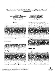
4. Examples of the application of the proposed algorithm To test the above described procedures two circuits were used: a simple design (24-port Register File with 72,000 transistors designed in 2.0 µm CMOS technology [13]) and a real life industrial design (more than 900,000 transistors, 0.8 µm CMOS technology). For both circuits a number of critical area functions were extracted. The results are discussed in this section. Fig. 30 shows the critical area for opens extracted for Metal 1, Metal 2, Poly, Active Area, Contact and Via layers for the Register File. Fig. 31 shows the same curves for small defect radii range. In both cases the critical areas for contacting regions were taken into account. Fig. 32 illustrates the relative error of critical area calculation for Metal 1, Metal 2, Poly and Active Area layers. This error was calculated as a difference between critical areas with and without contacting regions. It can be seen that the critical area for contacting regions plays a greater role in short and wide conducting paths, e.g. for the Active Area layer.

Ð 21 Ð


0.60

Critical Area for Opens [cm 2]

0.50 0.40 0.30 Metal 1 Metal 2 Poly

0.20

Active Area Contact Via

0.10 0.00 0

10

20

30 40 Defect Radius [µm]

50

60

Figure 30. Critical area for opens for Metal 1, Metal 2, Poly, Active Area, Contact and Via layers. 0.5

Metal 1 Metal 2 Poly Active Area


0.4

0.3

Contact Via

0.2

0.1

0.0 0

1

2


5

6

Figure 31. Critical area for opens for Metal 1, Metal 2, Poly, Active Area, Contact and Via layers for defect radius range 0 - 6 µm. Critical area for contacting regions is taken into account.

Ð 22 Ð


Relative Error of Critical Area Calculation [%]

100 90 80

Metal 1 Metal 2 Poly Active Area

70 60 50 40 30 20 10 0 -10 0

1

2


5

6

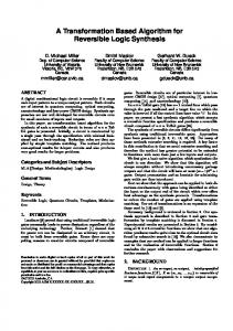
Figure 32. The difference between critical areas when the critical area for contacting regions is taken or not taken into account. For completeness of the IC layout analysis, the critical area for shorts for the same design is shown in Fig. 33. Notice the strong resemblance between these curves and the curves for the opens. Such a resemblance should be explored in the future for possible improvements in critical area extraction.

Critical Area for Shorts [cm 2]

0.60 0.50 0.40 0.30 Metal 1 Metal 2 Poly Active Area

0.20

0.10 0.00 0

10

20


50

60

Figure 33. Critical area for shorts for Metal 1, Metal 2, Poly and Active Area layers.

Ð 23 Ð


As it was mentioned the proposed algorithm was also used to extract critical areas for opens for the layout of a real life industrial design. The extracted data is shown in Fig. 34.


1.5

1.0

Metal 1 0.5

Metal 2 Poly Active Area Contact Via

0.0 0.0

1.0

2.0

3.0

4.0

5.0

6.0

7.0

8.0

9.0

10.0

Defect Radius [µm]

Figure 34. Critical area for opens in the real life industrial design. The above data was extracted by implementing the algorithm described in this paper using CADENCE Dracula [14]. Table 1 shows a summary of extraction time for the data shown in Fig.Ê31 and Fig. 34. Table 1.

The extraction time for the data shown in Fig. 31 and Fig. 34 ( m Ð minutes, h Ð hours ).

Design

Metal 1

Metal 2

Poly

Active

Contact

Via

Total

24 ÐPort Register File

55.6 m

7.0 m

13.4 m

39.5 m

22.3 m

2.8 m

140.6 m

Industrial Design

72.14 h

16.41 h

17.43 h

20.5 h

7.43 h

2.45 h 136.36 h

5. Conclusions In this paper a new algorithm for the extraction of the critical area for opens has been presented. In this algorithm the critical area for conducting paths and for electrical contacts to the other conducting layers are taken into account. The new concept of the contact or via contacting regions was introduced and its relevance was discussed. In contrast to other work, the proposed

Ð 24 Ð


algorithm allows analysis of large ICs and ICs with non-Manhattan geometry. An illustrative example shows that the extraction of critical areas for opens can be done for VLSI circuits of realistic size in a reasonable time.

Appendix: Procedure approximating Shrink operation Since a shrink operation, such as the one described in the body of the paper, is not always available there exists a need to approximate this operation by using the Òdown sizingÓ operation commonly found in mask fracturing tools. This appendix describes such an approximating procedure. A direct application of the Òdown sizingÓ operation in a shrink function is not possible because Òdown sizingÓ is not able to produce Negative polygons (see Sec. 3.1). So in order to construct the Shrink function one must first develop a simple way of generating an approximation to Negative polygons by using the Òdown sizingÓ operation. A possible solution for the approximation becomes apparent based on the following observation. Consider two long conducting path, P1 and P 2, of the same layer, with path width of W 1 and W2, respectively. Let d represent a small number2. (See Fig. A1.)

W1

W2 Path 2 (P2)

Path 1 (P1)

Figure A1. Example of conductive paths. First observe that the critical area contour produced by a Shrink operation on P1 for a defect radius of (

W1 + d ), which normally would produce a negative polygon, can be approximated by 2

the contour produced by shrinking P1 by ( 2

W1 - d ) (see Fig. A2)3. 2

In our implementation, d was set to the smallest resolution allowed by the DRC tool, 0.001 µm.

Ð 25 Ð


W1 - d 2

A AA

AA AA AA

Path 1 (P1)

W1 +d 2

Critical area of Path 1

Figure A2. Approximating Shrink operation. Note that the error of such this approximation, which is due to the ends of the critical area

AAAAAAAA AAAAAAAA AAAAAAAA AAAAAAAA AAAAAAAA AAAAAAAA AAAAAAAA AAAAAAAA AA AA

contours (see Fig. A3), is small if d is small and the connection is long.

d

2d

d

Shrink result

Error

Approximated result

Original contour

Figure A3. Error in approximation to Negative polygon.

Note also that critical area calculation can be done incrementally. Simply, if it is necessary to compute the critical area CA(R2) for a radius R 2 , when the critical area CA(R1), for R 1 with R2Ê>ÊR1 is already known, one can grow CA(R1) by R2 Ð R1. In our example (Fig. A1) the above observation means that for W1 < W2 , the portion of the critical area contour generated by a Shrink W2 can be calculated by oversizing the critical area contour of P1 at 2 W W W the defect radius 1 by the difference in radii ( 2 - 1 ). Figs. A4a and A4b show the critical area 2 2 2 W2 W1 of P1 at defect radii and , respectively. Fig. A4c shows the critical area of P1 at defect 2 2 W W W radius 2 over sized by ( 2 - 1 ). 2 2 2

operation on P1 at defect radius

3

This observation is only valid for paths of fixd width. What is done for paths of varying width is described at the end of this section in detail.

Ð 26 Ð


A AA AA AA AA AA AA

W1 2

W2 2

(a)

(b)

A A A A A

AA AA AA

W2 - W1 2 2

Path 1 (P1)

(c)

Critical area of Path 1

Figure A4. Incremental computation of the critical area.

Notice that first of the above observation is only valid for paths of fixed width. To approximate the Shrink operation, we used the above observations and generate the results incrementally, using the contours of smaller defect radii to generate the contours of larger radii. The pseudo code replacing the command Shrink is: ¥ Pseudo Code A1 OverSize (SEED, (Ri Ð R(i-1) Ð d)) ® tmp5

/* Line 1 */

/**** Update SEED ****/ OverSize (tmp5, d) ® tmpA

/* Line 2 */

UnderSize (CMF, (Ri Ð d)) ® tmpB

/* Line 3 */

UnderSize (CMF, Ri) ® tmpC

/* Line 4 */

OverSize (tmpC, d) ® tmpD

/* Line 5 */

tmpB Ç tmpD ® tmpE

/* Line 6 */

tmpA È tmpE ® SEED

/* Line 7 */

Recall that the layer tmp5 will be combined with the critical area of contacting regions of the contacts, tmp3 (see Pseudo Code 3). In the above code, R i and R(i-1) denote the current and previous defect radius, respectively. The critical area contour SEED is empty, at the first iteration, because the critical area for defects of 0 radius for a path of any width is 0. In the subsequent iterations, SEED contains the critical area contour of a defect radius R(i-1) + d (see Fig. A5).

Ð 27 Ð


AAAAAAAA AAAAAAAA AAAAAAAAAAAA AAAAAAAAAAAA AAAAAAAAAAAAAA AAAAAAAAAAAAAA AAAAAAA AAAAAAA AAAAAAAAAAAAAAAA Metal 1 (CMF)

Critical Area Contour of R(i-1) + d (SEED)

Figure A5. Critical area SEED of a defect radius R(i-1) + d.

Line 1. OverSize (SEED, (Ri Ð R(i-1) Ð d)) ® tmp5 This instruction ÒgrowsÓ the SEED by Ri Ð R(i-1) Ð d, so the resulting critical area in tmp5 is

AAAAAAAA

for defect a radius Ri (see Fig. A6).

AA

Critical Area Contour of Ri (tmp5)

Critical Area Contour of R(i-1) + d (SEED)

Figure A6. Example of OverSize (SEED, (Ri Ð R(i-1) Ð d)) ® tmp5.

Note: All of the remaining instructions set up the extraction of the next defect radius. If there are no more defect radii to extract, then the extraction is complete. To prepare for the extraction of next defect radius, we will construct the critical area polygons for defect radius R i + d . The critical area polygons for defect radius R i + d is constructed from combining two set of polygons. One set is generated by simply expanding the critical area polygons of defect radius R(i-1) + d. This is accomplished through line 1 and 2 of the pseudo code above. The second set of polygons is generated by series of commands, line 3 to 6, designed to identify and isolate those portions of the original mask that has a width of 2Ri.

Ð 28 Ð


Line 2. OverSize (tmp5, d) ® tmpA This instruction ÒgrowsÓ the critical area contour tmp5 (for defect radius R i,), by d (see Fig. A7).

AAAAAAAA AA AA AA AA d

Critical Area Contour of Ri (tmp5) Expanded Contour (tmpA)

Figure A7. Example of OverSize (tmp5, d) ® tmpA.

Line 3. UnderSize (CMF, (Ri Ð d)) ® tmpB This instruction shrinks the input mask CMF by (Ri Ð d ), only features of width greater

AAA AAAAAAAAAAAA AAAAAAAAA AAA AAAAAAAAAAAA A AAAAAAAAAAAA AAAAAAAAAAAAAA AAAAAAAAAAAAAA AA A A

than 2 (Ri Ð d) are represented in the resulting contour (see Fig. A8). 2d

Metal 1 (CMF)

Temporary layer (tmpB)

Figure A8. Example of UnderSize (CMF, (Ri Ð d)) ® tmpB.

Line 4. UnderSize (CMF, Ri )® tmpC This instruction shrinks the input mask by R i. Features of width less than 2Ri are now removed from the resulting contour. This operation is used to find those features that have

Ð 29 Ð


a width greater than 2Ri (see Fig. A9). Note that features with a width slightly smaller than 2Ri (by 2d) are still in tempB.

AAAAAAAAAAAAA AAAAAAAA AAAAAAAAAAAAA A AAAAAAAAAAAAAA AAAAAAAAAAAAAA AAAAAAA AAAAAAA AA AAAAAAA AA AAAAAAA AA AA Ri

Ri

Metal 1 (CMF)

Temporary layer (tmpC)

Figure A9. Example of UnderSize (CMF, Ri )® tmpC.

Line 5. OverSize (tmpC, d) ® tmpD This instruction ÒgrowsÓ tmpC by d (see Fig. A10).

AAAA AA AAAA AA AAAA AA AAAAAA

Temporary layer (tmpC)

Temporary layer (tmpD)

Figure A10. Example of OverSize (tmpC, d) ® tmpD. Line 6. tmpB Ç tmpD ® tmpE This instruction is used to mask out all of the features of the layout in tmpB, with a feature size larger than 2Ri (see Fig. A11).

A A

Temporary layer (tmpB)

Temporary layer (tmpD)

Temporary layer (tmpE) Figure A11. Example of tmpB Ç tmpD ® tmpE.

Ð 30 Ð


Line 7. tmpA È tmpE ® SEED This function combines the newly formed ÒseedsÓ and combine them with the existing contours in the SEED layer. The result is the critical area for the defect radius R i + d (seeÊFig. A12). Temporary layer (tmpE) Combined with (È):

Critical Area Contour of Ri Expanded by d (tmpA)

AA A AAAAAAAAAAAA AA A AAAAAAAAAAAAAA AAAAAAAAAAAAAA AAAAAAA AAAAAA AAAAAAAAAAAAA Critical Area Contour of Ri + d (SEED)

Figure A12. Example of tmpA È tmpE ® SEED. The approximation described above can only be used for paths of fixed width Tapered path, such as the one shown in Fig. A13, will have to be approximated by using segments of fixed width (see Fig. A14).

Figure A13. Tapered path.

Ð 31 Ð


R(i+3)

R(i+2)

R(i+1)

Ri

Figure A14. Approximating path in Fig. A13. The accuracy of the approximation will depend on the number of used. More segments make the estimation more accurate. However, when more segments are used a greater number of calculations at different defect radii is needed to perform an accurate extraction. (Fig. A14 shows an example with four defect radii, R i, R i+1, R i+2, R i+3.) So, a trade-off between accuracy and extraction time exists in a case of tapered paths.

Acknowledgments The authors would like to thank Dr. P. K. Nag and Dr. H. T. Heineken, T. Vogels, and K.ÊRyu for valuable feedback. References [1] W. Maly and J. Deszczka, ÒYield estimation model for VLSI artwork evaluation,Ó Electronics Letters, vol. 19, no. 6, pp. 226-227, March 1983. [2] W. Maly, ÒModeling of lithography related yield losses for CAD of VLSI circuits,Ó IEEE Trans. Computer-Aided Design, vol. 4, no. 3, pp. 166-177, July 1985. [3] D. M. H. Walker and S. W. Director, ÒVLASIC: A catastrophic fault yield simulator for integrated circuits,Ó IEEE Trans. Computer-Aided Design, vol. 5, no. 4, pp. 541-556, Oct. 1986. [4] J. Pineda de Gyvez and C. Di, ÒIC defect sensitivity for footprint-type spot defects,Ó IEEE Trans. Computer-Aided Design, vol. 11, no. 5, pp. 638-658, May 1992. [5] G. A. Allan, A. J. Walton, ÒHierarchical critical area extraction with the EYE tool,Ó Proc. of IEEE International Workshop on Defect and Fault Tolerance in VLSI Systems, pp. 28-36, Lafayette, USA, Nov. 1995. [6] I. A. Wagner, I. Koren, ÒAn interactive VLSI CAD tool for yield estimation,Ó IEEE Transactions on Semiconductor Manufacturing, vol. 8, no. 2, pp. 130-138, May 1995. [7] W. A. Pleskacz, ÒThe analysis of influence of layout disturbances on the performance and manufacturing yield of VLSI circuits,Ó Ph.D. Dissertation (in Polish), Warsaw University of Technology Ð Institute of Microelectronics and Optoelectronics, Warsaw, Oct. 1994.

Ð 32 Ð


[8] W. A. Pleskacz and W. B. Kuzmicz, ÒSENSAT Ð a practical tool for estimation of the IC layout sensitivity to spot defects,Ó The European Design and Test Conference EDAC-95, Paris, March 1995. [9] P. K. Nag and W. Maly, ÒHierarchical extraction of critical area for shorts in very large ICs,Ó Proc. of IEEE International Workshop on Defect and Fault Tolerance in VLSI Systems, pp. 10-18, Lafayette, USA, Nov. 1995. [10] I. Bubel, W. Maly, T. Waas, P. K. Nag, H. Hartmann, D. Schmitt-Landsiedel and S . Griep, ÒAFFCCA: a tool for critical area analysis with circular defects and lithography deformed layout,Ó Proc. of IEEE International Workshop on Defect and Fault Tolerance in VLSI Systems, pp. 19-27, Lafayette, USA, Nov. 1995. [11] W. Maly, M. E. Thomas, J. D. Chinn and D. M. Campbell, ÒMeasurements of type, size and density of spot defects,Ó in Design for Yield edited by W. R. Moore, W. Maly and A. J. Strojwas. Bristol and Boston: Adam Hilger, 1988. [12] J. B. Khare, W. Maly, S. Griep and D. Schmitt-Landsiedel, ÒYield-oriented computeraided defect diagnosis,Ó IEEE Transactions on Semiconductor Manufacturing, vol. 8, no. 2, pp. 195-206, May 1995. [13] W. Maly, M. Patyra, A. Primatic, V. Raghavan, T. Storey and A. Wolfe, ÒMemory chip for 24-port global register file,Ó Proc. of IEEE Custom Integrated Circuits Conference, San Diego, May 1991. [14] Cadence Opus Integrated Design Environment, Reference Manual Set. San Jose, CA: Cadence Design Systems Inc., 1994. [15] F. Preparata, M. Shamos, Computational Geometry - An Introduction. New York: Springer-Verlag, 1985, pp. 345-350. [16] C. H. Ouyang, W. A. Pleskacz and W. Maly, ÒExtraction of Critical Areas for Opens in Large VLSI Circuits,Ó CMU-SRC Research Report No. CMUCAD-96-18, Pittsburgh, USA, June 1996. [17] C. H. Ouyang, W. A. Pleskacz and W. Maly, ÒExtraction of Critical Areas for Opens in Large VLSI Circuits,Ó Proc. of IEEE International Symposium on Defect and Fault Tolerance in VLSI Systems, pp. 21-29, Boston, USA, Nov. 1996. [18] U. Lauther, ÒAn O(N log N) Algorithm for Boolean Mask OperationsÓ, Proc. of 18-th Design Automation Conference, pp. 555-560, USA, 1981.

Ð 33 Ð

A DRC Based Algorithm for Extraction of Critical ... - Semantic Scholar

A DRC Based Algorithm for Extraction of Critical ... - Semantic Scholar

Suggest Documents

AN EFFICIENT ALGORITHM FOR EXTRACTION ... - Semantic Scholar

A Synchronization Based Algorithm for ... - Semantic Scholar

An Algorithm for Automatic Extraction of Canyons - Semantic Scholar

Evolutionary Algorithm Based Approach for ... - Semantic Scholar

Decomposition based Algorithm for State ... - Semantic Scholar

GENETIC ALGORITHM BASED SOLUTION FOR ... - Semantic Scholar

A Web-Based Isosurface Extraction System for ... - Semantic Scholar

A Modified SDS-Based DNA Extraction Method for ... - Semantic Scholar

Ontology-based semantic concept extraction - Semantic Scholar

A Fast and Robust 3D Feature Extraction Algorithm ... - Semantic Scholar

an efficient algorithm for motivic pattern extraction based on a ...

A new algorithm for interconnect capacitance extraction based on ... - LIX

A Transformation Based Algorithm for Reversible ... - Semantic Scholar

Genetic Algorithm based Input Selection for a ... - Semantic Scholar

RDB-MINER: A SQL-Based Algorithm for Mining ... - Semantic Scholar

A URL-String-Based Algorithm for Finding WWW ... - Semantic Scholar

A chain-cluster based routing algorithm for ... - Semantic Scholar

A New Sampling-Based Algorithm for Discovering ... - Semantic Scholar

A Position Based Ant Colony Routing Algorithm for ... - Semantic Scholar

A Change Information Based Fast Algorithm for ... - Semantic Scholar

A GA-Based Clustering Algorithm for Large Data ... - Semantic Scholar

A BDD-Based Polytime Algorithm for Cost ... - Semantic Scholar

Analysis on a mobile agent based algorithm for ... - Semantic Scholar

A Hybrid Kalman Filter Based Algorithm for Real ... - Semantic Scholar