A Fast Approximation-Guided Evolutionary Multi-Objective Algorithm

A Fast Approximation-Guided Evolutionary Multi-Objective Algorithm Markus Wagner and Frank Neumann Evolutionary Computation Group School of Computer Science The University of Adelaide Adelaide, SA 5005, Australia

ABSTRACT Approximation-Guided Evolution (AGE) [4] is a recently presented multi-objective algorithm that outperforms state-of-the-art multimulti-objective algorithms in terms of approximation quality. This holds for problems with many objectives, but AGE’s performance is not competitive on problems with few objectives. Furthermore, AGE is storing all non-dominated points seen so far in an archive, which can have very detrimental effects on its runtime. In this article, we present the fast approximation-guided evolutionary algorithm called AGE-II. It approximates the archive in order to control its size and its influence on the runtime. This allows for trading-off approximation and runtime, and it enables a faster approximation process. Our experiments show that AGE-II performs very well for multi-objective problems having few as well as many objectives. It scales well with the number of objectives and enables practitioners to add objectives to their problems at small additional computational cost.

Categories and Subject Descriptors I.2.8 [Artificial Intelligence]: Problem Solving, Control Methods, and Search—Heuristic Methods

Keywords Approximation, Evolutionary Algorithms, Multi-Objective Optimization

1.

INTRODUCTION

Almost all real-world optimization problems have multiple and conflicting objectives. Therefore, such multi-objective optimization (MOO) problems do not have a single optimal function value, but usually encounter a wide range of function values with respect to the different objective functions where one can not improve one objective without worsening another one. The set of all the different trade-offs according to a given set of objective functions is called the Pareto front of the underlying multi-objective optimization problem. Even for two objectives the set of these trade-offs can become exponential with respect to the given input for discrete

Permission to make digital or hard copies of all or part of this work for personal or classroom use is granted without fee provided that copies are not made or distributed for profit or commercial advantage and that copies bear this notice and the full citation on the first page. To copy otherwise, to republish, to post on servers or to redistribute to lists, requires prior specific permission and/or a fee. GECCO’13, July 6–10, 2013, Amsterdam, The Netherlands. Copyright 2013 ACM 978-1-4503-1963-8/13/07 ...$15.00.

optimization problems or even infinite in the case of continuous optimization. Evolutionary algorithms (as almost all other algorithms) for multi-objective optimization restrict themselves to a smaller set of solutions that should be a good approximation of the Pareto front. Often, researchers in the field of evolutionary multi-objective optimization do not use a formal notion of approximation. Evolutionary multi-objective optimization focus on two goals. The first one is to get to the Pareto front and the second one is to distribute the points along the Pareto front. The first goal is usually achieved by optimizing the multi-objective problems according to the underlying dominance relation, whereas the second goal should be reached by the diversity mechanism that is usually incorporated into the algorithm. There are different evolutionary algorithms for multi-objective optimization such as NSGA-II [7], SPEA2 [22], or IBEA [21], which try to achieve these goals by preferring diverse sets of non-dominated solutions. However, they do not use a formal notation of approximation, which makes it hard to evaluate and compare algorithms for MOO problems. Recently, approximation-guided evolution (AGE) [4] has been introduced, which allows to incorporate a formal notion of approximation into a multi-objective algorithm. This approach is motivated by studies in theoretical computer science studying multiplicative and additive approximations for given multi-objective optimization problems [5, 6, 9, 20]. Nevertheless, it is very flexible and can (in principle) work with any formal notion of approximation. In this field of evolutionary multi-objective optimization, the frequently used hypvervolume indicator [23] allows for a related approach, which is however much harder to understand with respect to its optimization goal [2, 12]. Furthermore, the theoretical studies on -dominance [15] follow similar ideas, but they have not lead to successful algorithms. The reason is that it does not adjust itself to the optimization problem, but it works with a pre-set value for the target approximation. The framework of AGE presented in [4] is adaptable, it works with a given formal notion of approximation, and it improves the approximation quality during its iterative process. As the algorithm cannot have complete knowledge about the true Pareto front, it uses the best knowledge obtained so far during the optimization process. The experimental results in [4] show that given a fixed time budget AGE outperforms current state-of-the-art algorithms in terms of the desired additive approximation, as well as the covered hypervolume on standard benchmark functions. In particular, this holds for problems with many objectives, which most other algorithms have difficulties dealing with. Despite its good performance, the runtime of AGE can suffer in many-dimensional objective spaces. New incomparable solutions are inserted unconditionally into AGE’s archive, independent

of how different they are. These unconditional insertions can lead to huge archives that consequently slow down the algorithm. We propose a fast and effective approximation-guided evolutionary algorithm called AGE-II. It is fast and performs well for problems with many as well as few objectives. It can be seen as a generalization of AGE, but it allows to trade-off archive size and speed of convergence. To do so, we adapt the -dominance approach [15] in order to approximate the different points seen so far during the run of the algorithm (for similar approaches see, e.g., [17, 18]). Furthermore, we change the selection of parents being used for reproduction such that the algorithm is able to achieve a better spread along the Pareto front. Our experimental results show that AGE-II is fast, highly effective and outperforms the bestknown approaches in terms of approximation quality measured by the additive approximation for problems up to 20 objectives. The outline of this paper is as follows. We introduce some basic definitions as well as the original AGE in Section 2. In Section 3 we introduce our algorithm. In Section 4 we showcase the computational speed-up. In Section 5 we report on our experimental investigations. Finally, we finish with some conclusions.

2.

MULTI-OBJECTIVE APPROXIMATION GUIDED EVOLUTION

We now formalize the setting of multi-objective optimization and summarize the approximation-guided evolution approach of [4].

2.1

Multi-objective optimization

In multi-objective optimization the task is to optimize a function f = (f1 , . . . , fd ) : S → Rd+ with d ≥ 2, which assigns to each element s ∈ S a d-dimensional objective vector. Each objective function fi : S 7→ R, 1 ≤ i ≤ d, maps from the considered search space S into the positive real values. Elements from S are called search points and the corresponding elements f (s) with s ∈ S are called objective vectors. Throughout this paper, we consider the minimization problems of d objectives. In multi-objective optimization the given objective functions fi are usually conflicting, which implies that there no single optimal objective vector. Instead of this the Pareto dominance relation is defined, which is a partial order. In order to simplify the presentation we only work with the Pareto dominance relation on the objective space and mention that this relation transfers to the corresponding elements of S. The Pareto dominance relation  between two objective vectors x = (x1 , . . . , xd ) and y = (y1 , . . . , yd ), with x, y ∈ Rd is defined as x  y :⇔ xi ≤ yi for all 1 ≤ i ≤ d. We say that x dominates y iff x  y. If x ≺ y :⇔ x  y and x 6= y holds, we say that x strictly dominates y as x is not worse than y with respect to any objective, and at least better with respect to one of the d objectives. The objective vectors x and y are called incomparable if x k y :⇔ ¬(x  y ∨ y  x) holds. Two objective vectors are therefore incomparable if there are at least two (out of the d) objectives where they mutually beat each other. An objective vector x is called Pareto optimal if there is no y = f (s) with s ∈ S for which y ≺ x holds. The set of all Pareto optimal objective vectors is called the Pareto front of the problem given by f . Note that the Pareto front is a set of incomparable objective vectors.

Even for two objectives the Pareto front might grow exponentially with respect to the problem size. Therefore, algorithms for multi-objective optimization usually have to restrict themselves to a smaller set of solutions. This smaller set is then the output of the algorithm. We make the notion of approximation precise by considering a weaker relation on the objective vectors called additive dominance. It is defined as x + y :⇔ xi +  ≤ yi for all 1 ≤ i ≤ d. Furthermore, we also define additive approximation of a set of objective vectors T with respect to another set of objective vectors S. D EFINITION 1. For finite sets S, T ⊂ Rd , the additive approximation of T with respect to S is defined as α(S, T ) := max min max (si − ti ). s∈S t∈T 1≤i≤d

We will use Definition 1 in order to judge the quality of a population P with respect to a given archive A. In this way, we have a measure on how good the current population is with respect to the search points seen during the run of the algorithm. Although, we are only using the notion of additive approximation, we would like to mention that our approaches can be easily adapted to multiplicative approximation. To do this, we only need to adjust the definitions accordingly. Note that this indicator is sensitive to outliers. We prefer this over taking the average of the approximations. The resulting indicator would become very similar to the generational distance [19], and it would lose its motivation from theory.

2.2

Approximation-Guided Evolution (AGE)

Definition 1 allows to measure the quality of the population of an evolutionary algorithm with respect to a given set of objective vectors. AGE [4] is an evolutionary multi-objective algorithm that works with this formal notion of approximation. It stores an archive A consisting of the non-dominated objectives vectors found so far. Its aim is to minimize the additive approximation α(A, P ) of the population P with respect to the archive A. The experimental results presented in [4] show that given a fixed time budget it outperforms current state-of-the-art algorithms such as NSGA-II, SPEA2, IBEA, and SMS-EMOA in terms of the desired additive approximation, as well as the covered hypervolume on standard benchmark functions. In particular, this holds for problems with many objectives, which most other algorithms have difficulties dealing with. Quite surprisingly, it is the other way around when the problems have just very few objectives. As can be seen in Figure 5 (that will ) is clearly serve us for our final evaluation), the original AGE ( outperformed by other algorithms in several cases when the problem has just two to three objectives. We identified the following two important and disadvantageous properties of AGE: 1. A new but incomparable point is added to the archive independent of how different it is (see Line 10, Algorithm 3, [4])). These unconditional insertions can lead to huge archives that consequently slow down the algorithm. In Section 3.1, we introduce a technique to approximate the set of incomparable solutions seen. 2. The parents for the mating process are selected uniformly at random (see Line 6, Algorithm 3, [4])). Interestingly, this random selection does not seem to be detrimental to the algorithm’s performance on problems with many objectives.

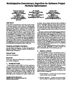
f2

Algorithm 1: Outline of AGE-II 3 · grid

Initialize population P with µ random individuals; Set grid the resolution of the approximative archive Agrid ; foreach p ∈ P do Insert offspring floor (p) in the approximative archive Agrid such that only non-dominated solutions remain;

1 2 3 4

2 · grid

foreach p ∈ O do Insert offspring floor (p) in the approximative archive Agrid such that only non-dominated solutions remain; Discard offspring p if it is dominated by any point increment(a), a ∈ A;

11 12

13

Add offsprings to population, i.e., P ← P ∪ O; while |P | > µ do Remove p from P that is of least importance to the approximation (for details on this step see [4]);

14 15 16

Algorithm 2: Function floor input : d-dimensional objective vector x, archive parameter grid output: Corresponding vector v on the -grid k j x[i] ; 1 for i = 1 to d do v[i] ←  grid

Algorithm 3: Function increment input : d-dimensional vector x, archive parameter grid output: Corresponding vector v that has each of its components increased by 1 1

for i = 1 to d do v[i] ← o[i] + 1 ;

However, realizing that the selection process might be improved motivated us to investigate algorithm-specific selection processes (see Section 3.2). Of course, it is not clear whether approximating the archive gives an approximation of the Pareto front. However, the intuition is that after some time the archive approximates the front quite well, so that an approximation of the archive directly yields an approximation of the front. The experiments presented later-on show that this intuition is right, as our algorithm indeed finds good approximations of the fronts.

grid

Q

nt

9 10

Q

ro

7 8

A

of

6

P

ret Pa

foreach generation do Initialize offspring population O ← ∅; for j ← 1 to λ do Select two individuals from P (see Section 3.2); Apply crossover and mutation; Add new individual to O;

5

R R

P

grid

f1 2 · grid

3 · grid

4 · grid

Figure 1: The newly generated points P , Q, and R are shown with their corresponding additive -approximations P , Q , and R . Both objectives f1 and f2 are to be minimised, and the current approximative archive is represented by . Only P will be added to the approximative archive, replacing A. Both P and Q will be candidates for the selection process to form the next population. that is similar to the original problem of multi-objective optimisation: a set of solutions is sought that nicely represents the true set of compromise solutions. In order to achieve this, we reuse AGE’s own main idea of maintaining a small set that approximates the true Pareto front. By approximating the archive as well in a controlled manner, we can guarantee a maximum size of the archive, and thus prevent the archive from slowing down the selection procedure. We achieve this based on the idea of -dominance introduced in (author?) [15]. Instead of using an archive At that stores at any point in time t the whole set of non-dominated objective vectors, we are (t) using an archive Agrid that stores an additive -approximation of the non-dominated objective vectors produced until time step t. In order to maintain such an approximation during the run of the algorithm, a grid on the objective space is used to pick a small set of representatives (based on -dominance). We reuse the update(t) mechanism from [15], and thus can maintain the -Pareto set Agrid of the set A(t) of all solutions seen so far. Due to [15], the size is bounded by m−1 Y  K  (t) Agrid ≤ grid j=1 where

  d K = max max fi (s) i=1

s∈S

In this section, we present our algorithm. We show how we adapt the -dominance approach (author?) [15] in order to approximate the different points seen so far during the run of the algorithm. Subsequently, we motivate our parent selection strategy.

is the maximum function value attainable among all objective functions. Our new algorithm called AGE-II is parametrized by the desired approximation quality grid ≥ 0 of the archive with respect to the seen objective vectors. AGE-II is shown in Algorithm 1, and it uses the helper functions given in Algorithms 2 and 3. The latter is used to perform a relaxed dominance check on the offspring p in Line 13. A strict dominance check here would require an offspring to be not dominated by any point in the entire archive. However, as the archive approximates all the solutions seen so far (via the flooring), it might very unlikely, or even impossible, to find solutions that pass the strict dominance test.

3.1

3.2

3.

AGE-II

Archive Approximation

The size of the archive can grow to sizes that slow down the original AGE tremendously. Interestingly, we are thus facing a problem

High Performance for Lower Dimensions

Quite interestingly, and despite AGE’s good performance on problems with many objective, it is clearly outperformed by other

algorithms in several cases, when the problem has just two or three objectives. The key discovery is that the random parent selection of AGE is free of any bias. For problems with many objectives, this is not a problem, and can even be seen as its biggest advantage. For problems with just a few objectives, however, it is well known that one can do better than random selection, such as selection based on crowding distance, hypervolume contribution, etc. Such strategies then select potential candidates based on their relative position in the current population. For AGE, the lack of this bias means that solutions can be picked for parents that are not necessarily candidates with high potential. Consequently, it is not surprising to see that the original AGE is outperformed by algorithms that do well with their parent selection strategy, if their strategy is effective in the d-dimensional objective space. Based on the previous experiments, we choose the following parent selection strategy for the final comparison against the established algorithms. Firstly, the population is reduced: solutions in the front i have a probability of 1/i of staying in the population. Secondly, a binary tournament on two randomly selected solutions from the reduced pool is performed for the parent selection, where solutions of higher crowding distance are preferred. The consequence of the reduction is that all solutions that form the first front are kept in the population, so are the extreme points. Additionally, solutions that are dominated multiple times are less likely to be selected as a potential parent. The use of the crowding distance then helps with maintaining a diverse set of solutions in low-dimensional objective space. Both steps taken together significantly increase the selection pressure over the original random selection in AGE. At the same time, they are quick to compute and their effects diminish when the number of objectives increases.

4.

SPEED-UP THROUGH APPROXIMATIVE ARCHIVES (t)

AGE-II works at each time step t with an approximation Agrid of the set of non-dominated points At seen until time step t. Note, that setting grid = 0 implies the original AGE approach that stores every non-dominated objective vector. In this section, we want to investigate the effect of working with different archives sizes (determined by the choice of grid ) in AGE-II. Our goal is to understand the effect of the choice of this parameter on the actual archive size used during the run of the algorithm as well as on the approximation quality obtained by AGE-II. Next, we outline the results of our experimental investigation of the influence of approximative archives on the runtime and the solution qualities. Note, that the computational complexity of the original AGE is linear in the number of objectives, and this holds for AGE-II, too. The algorithm was implemented in the jMetal framework [10] and is publicly available1 . The parameter setup of AGE-II is as follows. As variation operators, the polynomial mutation and the simulated binary crossover [1] were applied, which are both used widely in MOO algorithms [7, 13, 22]. The distribution parameters associated with the operators were ηm = 20.0 and ηc = 20.0. The crossover operator is biased towards the creation of offspring that are close to the parents, and was applied with pc = 0.9. The mutation operator has a specialized explorative effect for MOO problems, and was applied with pm = 1/(number of variables). Population size was set to µ = 100 and λ = 100, and each setup was given a budget of 100,000 evaluations. We assess the selection schemes and algorithms using the additive approximation measures ([4]): we approximate the achieved additive approximation of the known 1

http://cs.adelaide.edu.au/~ec/research/age.php

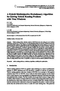
Pareto fronts by first drawing one million points of the front uniformly at random and then computing the additive approximation that the final population achieved for this set. Figure 2 shows the results averaged over 100 independent runs. Note how different the archive growth is for the different selected functions in the cases of grid = 0, where every non-dominated point is stored. For DTLZ 1, d = 2 the archive stays very small, with about 80 solutions in the end. Even in the case of DTLZ 3, d = 10 (a function with a similar objective space to that of DTLZ 1) only about every tenth solution is kept in the archive, which eventually contains about 9,000 solutions. For the similar objective spaces of DTLZ 2, d = 3 and DTLZ 4, d = 20 this situation is significantly different, and the rate of producing non-dominated points is significantly higher. In the case of the latter, over 90% of all generated solutions are added to the archive, if the insertion is just based on non-dominance. This situation changes only slightly, when a relatively "coarse" grid = 0.1 is used. For DTLZ 3, d = 10, the same value of the grid results in an enormous reduction in archive size. Consequently, the choice of grid has a significant impact on the runtime and even on the solution quality. For DTLZ 1, d = 2 the quality of the final population can be increased, whereas the use of an approximative archive has little impact on the archive size in this case. Of the tested values for DTLZ 2, d = 3 the choice of grid = 0.01 offers a speed-up by a factor of eight. Additional speed-ups can be achieved, but they come at the cost of worse final approximations. For DTLZ 3, d = 10 a similar observation can be made: if a minor reduction in quality is tolerable, then a speed-up by a factor of four can be achieved. The situation is very different for the 20-dimensional DTLZ 4, where a speed-up by a factor of over 250 can be achieved, while achieving even better quality solutions as well.

5.

BENCHMARK RESULTS

In this section, we compare AGE-II to well know evolutionary multi-objective algorithms including the original AGE on commonly used benchmark functions.

5.1

Experimental Setup

We use the jMetal framework [10] to compare our AGE-II with the original AGE, and with the established algorithms IBEA [21], NSGA-II [7], SMS-EMOA [11], and SPEA2 [22] on the benchmark families WFG [14], LZ [16], and DTLZ [8]. The test setup is identical to that of [4], and to the already outlined setup of Section 4. It is important to note that we limit the calculations of the algorithms to a maximum of 50,000/100,000/150,000 fitness evaluations for WFG/DTLZ/LZ and to a maximum computation time of 4 hours per run, as the runtime of some algorithms increases exponentially with respect to the size of the objective space. The further parameter setup of the algorithms is as follows. Parents were selected through a binary tournament (unless further specified). We will present our results for population size µ = 100 and λ = 100, averaged over 100 independent runs. We assess the algorithms by taking their final populations, and then using the afore-described additive approximation measure and the hypervolume [23]. The latter is a popular performance measure that measures the volume of the dominated portion of the objective space relative to a reference point r. For the quality assessment on the WFG and LZ functions, we computed the achieved additive approximations and the hypervolumes with respect to the Pareto fronts given in the jMetal package. For DTLZ 1 we choose r = 0.5d , otherwise r = 1d . We approximate the achieved hypervolume with an FPRAS [3], which has a relative error of more

DTLZ 1, d=2

DTLZ 2, d=3

archive size

grid = 0 : t = 13, a = 1.55 grid = 0.01 : t = 14, a = 0.68 grid = 0.1 : t = 13, a = 0.78 grid = 1.0 : t = 12, a = 1.94 grid = 10.0 : t = 13, a = 3.90

100

archive size

grid = 0 : t = 578, a = 0.05 grid = 0.001 : t = 600, a = 0.05 grid = 0.01 : t = 74, a = 0.05 grid = 0.1 : t = 14, a = 0.10 grid = 1.0 : t = 12, a = 0.56

20,000

DTLZ 3, d=10

95,000

85,000

evaluations

DTLZ 4, d=20

archive size

grid = 0 : t = 215, a = 0.50 grid = 0.01 : t = 239, a = 0.57 grid = 0.1 : t = 177, a = 0.53 grid = 1.0 : t = 48, a = 0.57 grid = 10.0 : t = 19, a = 3.80

8,000

archive size

grid = 0 : t = 5336, a = 0.27 grid = 0.1 : t = 4697, a = 0.26 grid = 0.2 : t = 803, a = 0.23 grid = 0.3 : t = 21, a = 0.26 grid = 0.4 : t = 19, a = 0.30

60,000

95,000

85,000

75,000

0

65,000

95,000

85,000

75,000

65,000

55,000

evaluations

55,000

30,000

4,000

0

75,000

0

65,000

95,000

85,000

75,000

65,000

55,000

evaluations

55,000

10,000

50

evaluations

Figure 2: Influence of grid on the archive size, the runtime, and the final quality. Shown are the means of the archive sizes, and their standard deviation is shown as error bars. Additionally, the means of the runtime t in seconds and the achieved additive approximation a of the true Pareto front are listed (smaller values are better). Note: the archive can grow linearly with the number of solutions generated, even when problem have just d = 3 objectives. Furthermore, if the front is small compared to the volume of the objective space (see DTLZ 1 and 3), then the archive can grow and shrink during the optimisation. than 2% with probability less than 1/1000. The volumes shown for DTLZ 1 are normalized by the factor 2d . As it is very hard to determine the minimum approximation ratio achievable or the maximum hypervolume achievable for all populations of a fixed size µ, we only plot the theoretical maximum hypervolume for µ → ∞ as a reference. Note that, by the design of the additive approximation indicator, the approximation values indicate the distributions of the solution and their distances from the Pareto front, as no point on the Pareto front is approximated worse than the indicator value.

5.2

Experiment results

The benchmarking results for the different algorithms are shown in Figures 3, 4, and 5. In summary, AGE-II ranks among the best algorithms on the low-dimensional WFG and LZ functions. This holds for both the additive approximation quality, as well as for the ) that norachieved hypervolumes. Interestingly, NSGA-II ( mally performs rather well on such problems, is beaten in almost all cases. SPEA2 ( ) and IBEA ( ) on average perform better. AGE ( ), SMS-EMOA ( ), and AGE-II (grid = 0.1 : , grid = 0.01 : ) often perform very similarly. Our investigations on the DTLZ family prove to be more differentiating. As these can be scaled in the number of objectives, the advantages and disadvantages of the algorithms’ underlying mechanisms become more apparent: • AGE-II (grid = 0.1 : , grid = 0.01 : ) shows a significantly improved performance on the lower-dimensional

DTLZ 1, DTLZ 3, and DTLZ 4 variants. Furthermore, it is either the best performing algorithm, or in many cases, it shows at least competitive performance. • It is interesting to see that our AGE-II incorporates the ) for a fitness crowding distance idea from NSGA-II ( assignment, but is not influenced by its detrimental effects in higher dimensional objective spaces. This is thanks to the way how the next generation is formed (i.e., based on contributions to the approximation achieved of the archive, see Line 16 of Algorithm 1). • When compared with the original AGE ( ), then our modification does exhibit a performance improvement in all cases. Still, as AGE-II shows a consistent performance across all scaled functions, we deem the minimal loss in quality (in our experimental setup) as negligible. ), SMS-EMOA ( ), and • Remarkably, NSGA-II ( SPEA2 ( ) are unable to find the front of the high-dimensional DTLZ 1 and DTLZ 3 variants. This results in extremely large approximations and zero hypervolumes. • The reason for IBEA’s decreasing behaviour for very large dimension (d ≥ 18) is that it was stopped after 4 hours and it could not perform 100, 000 iterations. The same holds already for much smaller dimensions for SMS-EMOA ( ), which uses an exponential-time algorithm to internally determine the hypervolume. It did not finish a single genera-

hypervolume for WFG 1-9, d = 2 (larger = better)

approximation for WFG 1-9, d = 2 (smaller = better)

100 100

10−1

10−2 2

3

4

5 6 function

7

8

10−2

9

hypervolume for for WFG 1-9, d = 3 (larger = better)

approximation for WFG 1-9, d = 3 (smaller = better)

1

100

10−1

10−2 1

2

3

4

5 6 function

7

8

10−1

9

1

2

3

4

5 6 function

7

8

9

1

2

3

4

5 6 function

7

8

9

100

10−1

10−2

Figure 3: Comparison of the performance of our AGE-II (grid = 0.1 : , grid = 0.01 : ) with the original AGE ( ), IBEA ( ), NSGAII ( ), SMS-EMOA ( ), and SPEA2 ( ) with varying dimension d. The figures show the average of 100 repetitions each. Only non-zero hypervolume values are shown.

100 hypervolume for LZ 1-9 (larger = better)

approximation for LZ 1-9 (smaller = better)

100

10−1

10−1 1

2

3

4

5 6 function

7

8

9

10−2

1

2

3

4

5 6 function

7

8

9

Figure 4: Comparison of the performance of our AGE-II (grid = 0.1 : , grid = 0.01 : ) with the original AGE ( ), IBEA ( ), NSGAII ( ), SMS-EMOA ( ), and SPEA2 ( ) with varying dimension d. The figures show the average of 100 repetitions each. Only non-zero hypervolume values are shown.

100 hypervolume for DTLZ 1 (larger = better)

approximation for DTLZ 1 (smaller = better)

103

101

10−1 2

4

6

8

10 12 14 dimension

16

18

10−1

10−2

20

2

4

6

8

10 12 14 dimension

16

18

20

2

4

6

8

10 12 14 dimension

16

18

20

hypervolume for DTLZ 2 (larger = better)

approximation for DTLZ 2 (smaller = better)

100 100

10−1

10−2 2

4

6

8

10 12 14 dimension

16

18

10−1

10−2

20

hypervolume for DTLZ 3 (larger = better)

approximation for DTLZ 3 (smaller = better)

100

102

100

2

4

6

8

10 12 14 dimension

16

18

10−1

10−2

20

2

4

6

8

10 12 14 dimension

16

18

20

hypervolume for DTLZ 4 (larger = better)

approximation for DTLZ 4 (smaller = better)

100

100

10−1

2

4

6

8

10 12 14 dimension

16

18

20

10−1

10−2

2

4

6

8

10 12 14 dimension

16

18

20

Figure 5: Comparison of the performance of our AGE-II (grid = 0.1 : , grid = 0.01 : ) with the original AGE ( ), IBEA ( ), NSGA-II ( ), SMS-EMOA ( ), and SPEA2 ( ) with varying dimension d. The figures show the average of 100 repetitions each. Only non-zero hypervolume values are shown. For reference, we also plot ( ) the maximum hypervolume achievable for µ → ∞.

tion for d ≥ 8 and only performed around 5, 000 iterations within four hours for d = 5. This implies that the higherdimensional approximations plotted for SMS-EMOA actually show the approximation of the random initial population. • Interestingly, the approximations achieved by NSGA) and SPEA2 ( ) are even worse as they are tuned II ( for low-dimensional problems and move their population too far out to the boundaries for high dimensions.

6.

CONCLUSIONS

Approximation guided evolutionary algorithms work with a formal notion of approximation and have the ability to work with problems of many dimensions. Our new approximation-guided algorithm called AGE-II efficiently solves problems with few and with many conflicting objectives. Its computation time increases only linearly with the number of objectives. We control the size of the archive which mainly determines its computational cost, and thus observed runtime reductions by a factor of up to 250 over its predecessor, without a sacrifice of final solution quality. Our experimental results show that given a fixed time budget it outperforms current state-of-the-art approaches in terms of the desired additive approximation on standard benchmark functions for more than four objectives. On functions with two and three objectives, it lies level with the best approaches. Additionally, it also performs competitive or better regarding the covered hypervolume, depending on the function. This holds in particular for problems with many objectives, which most other algorithms have difficulties dealing with. In summary, AGE-II is an efficient approach to solve multiproblems with few and many objectives. It enables practitioners now to add objectives with only minor consequences, and to explore problems for even higher dimensions.

References [1] R. B. Agrawal and K. Deb. Simulated binary crossover for continuous search space. Technical report, 1994. [2] A. Auger, J. Bader, D. Brockhoff, and E. Zitzler. Theory of the hypervolume indicator: optimal µ-distributions and the choice of the reference point. In Proc. 10th International Workshop on Foundations of Genetic Algorithms (FOGA ’09), pages 87–102. ACM Press, 2009. [3] K. Bringmann and T. Friedrich. Approximating the volume of unions and intersections of high-dimensional geometric objects. Computational Geometry: Theory and Applications, 43:601–610, 2010. [4] K. Bringmann, T. Friedrich, F. Neumann, and M. Wagner. Approximation-guided evolutionary multi-objective optimization. In Proc. 21nd International Joint Conference on Artificial Intelligence (IJCAI ’11), pages 1198–1203, Barcelona, Spain, 16-22 July 2011. IJCAI/AAAI. [5] T. C. E. Cheng, A. Janiak, and M. Y. Kovalyov. Bicriterion single machine scheduling with resource dependent processing times. SIAM J. on Optimization, 8:617–630, 1998. [6] C. Daskalakis, I. Diakonikolas, and M. Yannakakis. How good is the Chord algorithm? In Proc. 21st Annual ACMSIAM Symposium on Discrete Algorithms (SODA ’10), pages 978–991, 2010. [7] K. Deb, A. Pratap, S. Agrawal, and T. Meyarivan. A fast and elitist multiobjective genetic algorithm: NSGA-II. IEEE Trans. Evolutionary Computation, 6(2):182–197, 2002.

[8] K. Deb, L. Thiele, M. Laumanns, and E. Zitzler. Scalable test problems for evolutionary multiobjective optimization. In Evolutionary Multiobjective Optimization, Advanced Information and Knowledge Processing, pages 105–145. 2005. [9] I. Diakonikolas and M. Yannakakis. Small approximate Pareto sets for biobjective shortest paths and other problems. SIAM Journal on Computing, 39:1340–1371, 2009. [10] J. J. Durillo, A. J. Nebro, and E. Alba. The jMetal framework for multi-objective optimization: Design and architecture. In Proc. Congress on Evolutionary Computation (CEC ’10), pages 4138–4325. IEEE Press, 2010. [11] M. T. M. Emmerich, N. Beume, and B. Naujoks. An EMO algorithm using the hypervolume measure as selection criterion. In Proc. Third International Conference on Evolutionary Multi-Criterion Optimization (EMO ’05), pages 62–76. Springer, 2005. [12] T. Friedrich, C. Horoba, and F. Neumann. Multiplicative approximations and the hypervolume indicator. In Proc. 11th annual Conference on Genetic and Evolutionary Computation (GECCO ’09), pages 571–578. ACM Press, 2009. [13] M. Gong, L. Jiao, H. Du, and L. Bo. Multiobjective immune algorithm with nondominated neighbor-based selection. Evolutionary Computation, 16(2):225–255, 2008. [14] S. Huband, L. Barone, R. L. While, and P. Hingston. A scalable multi-objective test problem toolkit. In C. A. C. Coello, A. H. Aguirre, and E. Zitzler, editors, Evolutionary MultiCriterion Optimization, (EMO ’05), volume 3410 of LNCS, pages 280–295. Springer, 2005. [15] M. Laumanns, L. Thiele, K. Deb, and E. Zitzler. Combining convergence and diversity in evolutionary multiobjective optimization. Evolutionary Computation, 10(3):263–282, 2002. [16] H. Li and Q. Zhang. Multiobjective optimization problems with complicated pareto sets, MOEA/D and NSGA-II. IEEE Trans. on Evolutionary Computation, 13(2):284–302, 2009. [17] O. Schütze, M. Laumanns, C. A. C. Coello, M. Dellnitz, and E.-G. Talbi. Convergence of stochastic search algorithms to finite size pareto set approximations. Journal of Global Optimization, 41(4):559–577, 2008. [18] O. Schütze, M. Laumanns, E. Tantar, C. A. C. Coello, and E.-G. Talbi. Computing gap free pareto front approximations with stochastic search algorithms. Evolutionary Computation, 18(1):65–96, 2010. [19] D. A. Van Veldhuizen and G. B. Lamont. Multiobjective evolutionary algorithm research: A history and analysis. Technical report, Citeseer, 1998. [20] S. Vassilvitskii and M. Yannakakis. Efficiently computing succinct trade-off curves. Theor. Comput. Sci., 348:334–356, 2005. [21] E. Zitzler and S. Künzli. Indicator-based selection in multiobjective search. In Proc. 8th International Conference Parallel Problem Solving from Nature (PPSN VIII), volume 3242 of LNCS, pages 832–842. Springer, 2004. [22] E. Zitzler, M. Laumanns, and L. Thiele. SPEA2: Improving the strength Pareto evolutionary algorithm for multiobjective optimization. In Proc. Evolutionary Methods for Design, Optimisation and Control with Application to Industrial Problems (EUROGEN ’01), pages 95–100, 2002. [23] E. Zitzler and L. Thiele. Multiobjective evolutionary algorithms: a comparative case study and the strength Pareto approach. IEEE Trans. Evolutionary Computation, 3:257–271, 1999.