A Fast Design Model for Indoor Radio Coverage in the 2.4 GHz Wireless LAN Jaime Lloret, Jose J. López, Carlos Turró, Santiago Flores Department of Communications Universidad Politécnica de Valencia, Camino Vera s/n 46022 Valencia, SPAIN
[email protected]
Abstract—In this paper, an empiric radio coverage model for indoor wireless LAN is presented. This model has been tried out in a vast series of large extension buildings obtaining successful results. The objective of the model is to facilitate the radio design work of a wireless LAN by means of straightforward calculations, because the use of statistical methods is very time consuming, and difficult to put in practice at most situations. Our model is based on a derivation of the free field propagation equation taking into account the building structure and its materials and it has been tested on a large scale design of a WLAN network of over 400 access points. Finally, the paper includes the guidelines to setup a home, building, University campus, or city wireless LAN easily in three simple steps. Key Words-WLAN, wall loss, radio coverage, 802.11, 2.4 GHz
I.
INTRODUCTION
Since the launch of the wireless local area networks (WLAN) based on the 802.11b and 802.11g standard, a spectacular market growth has been experienced, due to the features offered and to the low costs of the necessary transmission equipment. Installation of one of these networks at home or in an office environment is straightforward, and technically affordable [1] [2] [3]. Nevertheless, when the requirements demanded to this network increase, for example, to cover a great area, more than one house or different floors in a building, the user has to face several technical limitations that require more in depth study of the installation. Additionally, this complication could increase a bit more when the full coverage a vast area with several buildings is needed. In this case, statistical models and ray tracing based methods are not always affordable. Furthermore, results of analytical and statistical methods can be unimplementable due to the real structure of the building and even to aesthetical considerations. On the other hand, wireless networks are widely developed around the world with interesting projects, sometimes promoted by the city councils that want to offer coverage to its neighbors, or by groups of users that want to establish their own particular network. There are many possibilities for using this unlicensed radio band technology, and simple models like the presented one, will be useful for these tasks. This paper is structured as follows: Section 2 describes the general approach of our model. Section 3 details the
calculations involved. Section 4 is devoted to the field testing and finally section 5 concludes the paper. II.
GENERAL APPROACH
The deployment of vast extension WLAN is faced with several problems. To develop a big project successfully, it is always necessary to use a smart work strategy from the very beginning that could minimize the design effort. We call that, “Design steps”, and will be applied to each building of the network. These steps are: 1) Visual study and inspection of the building through walking around them, and using its floor plan. 2) To carry out an initial set of measures to obtain an estimate of wall propagation losses. 3) Try a suitable location for each access point and carry out the calculations in order to estimate the coverage across the building, as a function of the obstructing walls in the light of sight and the distance to the access point. Step three is then repeated until a suitable location for all access points has been reached. Fig. 1 illustrates this approach. III.
WALL AND FLOOR PROPAGATION LOSSES
The three main mechanisms of radio propagation are attributed to reflection, diffraction, and dispersion. These three effects cause distortions in the radio signal that suffers attenuation due to losses in its propagation [4]. Common effects on the buildings that do not appear in free field are losses through the walls, roofs, and floors. This effect, together with the multipath and diffraction caused by the corners, is very difficult to evaluate, and there are many publications about mathematical models of indoor radio propagation [4] [5] [6]. The propagation losses value is given in equation (1), where the effect of the losses due to multipath effect is added [7] [8]: L(dB) = Lo+10n log(d)+ΣKiFi+ΣIjWj+Lms Where:
(1)
Figure 2. Consecutive walls used in the measurements, and check points for obtaining the mean loss through the walls of a building. Figure 1. Design step 1: Initial set of measures to estimate wall propagation losses.
Lo = power losses (dB) at a distance of 1m (40.2 dB at 2.44 GHz frequency) n = attenuation variation index with the distance (n=2) d = distance between transmitter and receiver Ki = number of floors of kind i in the propagation path Fi = attenuation of one floor of kind i. Ij = number of walls of kind j in the propagation path Wj = attenuation factor of one wall of kind j Lms = Propagation losses due to multipath propagation and light of sight interferences effect. There are a lot of studies devoted to the characterization of propagation losses through building materials (walls [10] [11] and floors [12]) or studies focused to solutions for specific buildings [13] [14]. It has also been demonstrated the dependence of the attenuation respect to the angle of interception with the wall or floor [15][16]. Nevertheless, from a practical design point of view, we will use simple statistical models of the wall’s absorption in order to predict how many walls the WLAN signal will be able to cross whilst maintaining connectivity. As shown on section four, this simple method will provide fairly good estimations. So, as stated in our general approach, we will begin by measuring the propagation loss of each type of wall in our environment. To do this, we will locate an area of consecutive walls (usually a corridor of office rooms) in the building, as shown in Fig. 1. According to Fig. 2, the transmitter is located at a fixed position ‘0’, 1 meter apart from the wall and a series of measures are taken at points 1-3-5-…-13 using a wireless card connected to a laptop, and signal monitoring software. Using equation (1) it is possible to calculate the loss through the first wall. L0-1 = Lo – 20 log (d) – Pr1 + Lms1
(2)
mean will be employed as a reference for all the walls of this type. Next table shows the values of attenuation obtained from a specific building. As can be seen, not all of the walls produce the same attenuation in spite of the fact that they are made from the same materials. This variation is produced by the multipath propagation and light of sight effects. By obtaining a mean value we reduce that source of error. Results can be seen on TABLE I. TABLE I.
Wall losses, and mean value.
Wall 0-1 2-3 4-5 Mean (Lp)
It is notable to remark that we obtain a value adjusted to that obtained on references [10] and [11], but using a very simple process. Now, we are ready to estimate the number of walls the wireless signal can cross without loss of connection. The deduced expression for the threshold power follows: Pu =Prx1m – 20 log (d) – ΣLipi
(3)
Where Lo = 40.2 dB and Pr2 is the received power at point ‘3’ and d = 4.5 meters in this case (wall separation is 2.5 meters for all rooms). So, to obtain a suitable value without multipath propagation losses we compute a mean value. This
(4)
Prx1m = Power received at 1meter d = Distance between the transmitter and the receiver ΣLipi = Propagation losses due to the walls of kind i The following expression can be used to obtain the number of walls that the signal can cross within a specific threshold power:
n=
Prx1m − 20 log d − Pu
Pr1 is the received power at point ‘1’ and d = 2 meters in this case. In order to compute the loss at the second wall: L2-3 = Lo – 20 log (d) – Pr3 – L0-1 + Lms2 - Lms1
Loss [dB] -1.021 15.352 2.802 5.711
∑LP
i i
(5)
And this other expression provides the maximum distance as a function of the number of crossed walls:
d = 10
Prx1 m − n ·
∑ Li Pi − Pu 20
(6)
Figure 3. Design step 2A: Attempts for a suitable access point location by estimation of the coverage across the building.
As an example of application, the TABLE II shows the maximum distance allowed as a function of the number of same type walls crossed by the signal. The power threshold is fixed at -80 dBm, which is the typical sensitivity value for the majority of commercial wireless LAN cards (at a transmission speed of 11 Mbps). TABLE II. Maximum distance allowed as a function of traversed walls.
1 wall 2 walls 3 walls 4 walls Distance (m) 50.64 14.19
13.60
7.05
It would be interesting to notice an irregular behavior in the signal attenuation when crossing a wall next to a toilet. Is this case, the loss caused by these walls is significantly greater than the caused by the rest of the walls in the building. This loss can be as great as 20 dB. The pipes embedded in the walls of these pieces probably cause this behavior. Consequently, special treatment of these walls can be taken in the computation of coverage of the building. As a rule of thumb placement of access points in the proximities of toilets must be avoided, so a big area of poor coverage will be created on the other side of the toilet (as it is shown in Fig. 3). Additionally it must be taken into account the metallic objects (rails, fences, statues, etc.) in the direct path, in these cases the measure suffers errors above +/-2 dB. Now, the building map and the wall losses mean value are only needed in order to design the coverage area as it is shown in Fig. 3 and Fig. 4. IV.
PRACTICAL VS THEORETICAL MEASUREMENTS
All the buildings on the campus of the Polytechnic University of Valencia have been studied. There are more than 50 buildings with quite a lot of floors spread over two square kilometers. It is understandable that different buildings built in different periods and with different building techniques will have different wall attenuation characteristics. Consequently, the study of wall loss would be made in each building of a extended area. So, in order to save field measures in all the campus buildings, they have been classified according to the building techniques and material employed for construction. A check on resemblances between the models and the real measures taken in the buildings was carried out. The validity
Figure 4. Design step 2B: Attempts for a suitable access point location by estimation of the coverage across the building.
of these models was confirmed. The TABLE III shows the results obtained for standard brick walls in different year-ofconstruction buildings: TABLE III. Attenuation mean value for different campus buildings.
Building Sports DCAN EUITI I3 DOEFFC 5I 5D 5E 1B Architecture 1E Computer Sc. Faculty 1F DSIC 1G EUI ETSA Block 2 ETSIA Block 3 3A – 2E 3M Fine Arts Mean value
Mean 7 5.25 6.41 6.12 6.47 6.33 6.53 6.6 5.83 6.81 7.35 6.32 4.66 5.62 5.19 8.21 6.29
A global mean value has also been obtained. It can be used in case of unknowing the model classification of the building. After obtaining the loss of signal power due to the wall, next step is to examine the building map to be covered with access points. With the obtained data, the wireless coverage can be designed from the far away points on the map. As shown in Fig. 5, the intersection between the cover zones designed will be the zone where the access point would be installed, Fig. 6. Now, in order to validate the model, a series of field measures has been taken in different points in the building and compared with the predicted ones using our model. As it is shown in TABLE IV, the error is comprised in the range between +/- 3dB, which should be enough for the majority of the situations. The standard deviation of the error is comprised between 1.6 and 1.9 dB, depending of the building. As illustration example, the measures obtained for two typical buildings between the 50 studied are shown.
Figure 5. Selection of the access point placement taking into account wall losses.
To assure a suitable reception for all wireless cards, we limit the power range at -80 dBm for 802.11b, and -68 dBm for 802.11g, so measures further from that point are not taken into account. The propagation signal between adjoining floors in a building is quite low, due to metal wrought between that acts as a front. Although if you are exactly above the AP of the inferior plant or vice versa, it is possible to receive a slight signal, and the signal attenuates quickly as soon as you go away. A good sign is only achieved between plants if the building has crystal skylights and the AP is located there. We have used our model in a 3D fashion to get a good estimate on these cases. On the other hand, the residual propagation between plants can cause interferences between channels in some points, so an appropriate 3D frequency planning is needed. To conclude, we present in Fig. 7 an example of the prediction maps obtained using the proposed model.
Figure 6. Access point placement and coverage area.
TABLE IV. Model prediction, compared with field measure and error, for two different buildings. Building A
Model predict. -63.88 -66.61 -76.19 -68.79 -79.62 -79.62 -77.24 -69.04 -73.89 -67.54 -77.84 -76.89 -77.00 -66.77 -68.27 -64.90 -68.44 -76.53 -76.95
Measured -62 -67 -79 -68 -79 79 -75 -71 -71 -64 -79 -74 -79 -68 -66 -64 -67 -77 -74
Model predict. -70.28 -76.19 -77.72 -75.16 -67.27 -73.73 -70.28 -74.61 -77.56 -74.57 -74.97 -63.93 -69.55 -77.47
Measured -73 -76 -78 -74 -65 -74 -69 -77 -76 -77 -78 -65 -67 -75
Error 1.88 -0.39 -2.81 0.79 0.62 0.62 2.24 -1,96 2.89 3.54 1.16 2.89 2.00 1.23 2.27 0.90 1.44 -0.47 2.95
Building B
Figure 7. Example of the prediction maps obtained using the proposed model: [-30,-50 dBm] ]-50,-70 dBm] ]-70,-80 dBm] < -80 dBm
Error -2.72 0.19 -0.28 1.16 2.27 -0.27 1.28 -2.39 1.56 -2.43 -3.03 -1.07 2.55 2.47
V.
CONCLUSIONS
An empiric radio coverage model for indoor wireless LAN based on a straightforward derivation of the free field propagation equation taking into account just the walls traversed has been presented and validated. This validation has been done extensively in different buildings built in different periods and with different building techniques. We have found that our model produces better approximations when the wall attenuation factor of a building is correctly selected from the database of constructive materials collected during the project. Nevertheless, this is not critical, and quite profitable and close to reality results can be obtained using a general value. It has been compared the predicted value respect to the measured one. The conclusion is that our model produce errors generally under +/- 3dB, with a standard deviation around 1.8 dB. An exhaustive and successfully campaign of field measures, on more than 50 building in the campus of the Universidad Politecnica de Valencia (Spain) guarantee its usability and employment in future projects. Our model has been used for the design of the wireless deployment using the standards 802.11b and 802.11g at our University campus. It is applicable to other Universities, office buildings, etc. ACKNOWLEDGEMENTS
We want to acknowledge all the students that participate in the exhaustive field measurement campaign for their valuable effort, and to the University Computer Center for their support in this initiative. REFERENCES [1]
Jeffrey Wheat, Designing a Wireless Network, Syngress Publishing, Rockland, 2001
[2] [3] [4]
[5]
[6] [7]
[8]
[9]
[10]
[11]
[12]
[13] [14] [15]
[16]
M.S. Gast, 802.11 wireless networks: the definitive guide, Ed. O'Reilly, Sebastopol, 2002 B. O'Hara, The IEEE 802.11 handbook: a designer's companion, IEEE Press, New York, 1999 C.C. Chiu and S.W. Lin, “Coverage prediction in indoor wireless communications”, IEICE Trans. Commun.,vol. E79-B,no.9,pp. 13461350,Sep. 1996 W.C. Chang, C.H. Ko, Y.H. Lee, S.T. Sheu, Y.J. Zheng, "A Novel Prediction System for Wireless LAN Based on the Genetic Algorithm and Neural Network", Proc. IEEE 24th Conference on Local Computer Networks, Oct. 1999, Lowell, Ma, USA Rappaport, Theodore S., Wireless Communications: Principles and Practice, Prentice Hall Publications, NJ, 1996. R. A. Valenzuela, "A Ray Tracing Approach to Predicting Indoor Wireless Transmission", IEEE Vehicular Technology Conference, Secaucus NJ, May 18-20, 1993, 214 – 218 T. Frühwirth, J.R. Molwitz and P. Brisset, “Planning Cordless Business Communication Systems”, IEEE Expert Magazine, Special Track on Intelligent Telecommunications, February 1996 F. Agelet, A. Formella, J. Rabanos, F. de Vicente and F. Fontan, “Efficient Ray-Tracing Acceleration Techniques for Radio Propagation Modeling”, IEEE Trans Vehicular Tech, 49 #6 p. 2069 John C. Stein, Indoor Radio WLAN Performance Part II: Range Performance in a Dense Office Environment, Harris Semiconductor (Intersil) Robert Wilson, Propagation Losses Through Common Building Materials 2.4 GHz vs 5 GHz. Magis networks Inc. http://www.magisnetworks.com/pdf/cto_notes/E10589PropagationLosse s.pdf D. Suwattana, J. Santiyanon, T. Laopetcharat, “Study on the Performance of Wireless Local Area Network in a Multistory Environment with 8-PSK TCM”, International Technical Conference On Circuits/ Systems, Computers and Communications J. S. Davis II, Measurements in Cory Hall at UC Berkeley. http://www.wireless.per.nl:202/multimed/cdrom97/2_4ghz.htm Dan Dobkin, Indoor Propagation and Wavelength, WJ Communications, 2002 http://www.wj.com/pdf/techpubs/Indoor_prop_and_80211.pdf R.F. Rudd, “building penetration loss for slant-paths at l-, s- and cband”, International Conference on Antennas and Propagation, March 2003 Adi Shamir; “An Introduction to Radio Waves Propagation: Generic Terms, Indoor Propagation and Practical Approaches to Path Loss Calculations, Including Examples”, RF Waves - White Paper. http://www.wtwo.net/testowo/rfwaves/