A fast implementation of kernel-based projection pursuit ... - CiteSeerX

A fast implementation of kernel-based projection pursuit indices Sigbert Klinke

Contents 1 2 3 4 5 6 7 A

Introduction Polynomial-based indices Kernel-based indices Binning Reducing to integer operations Conclusion Extensions C-Programs

A.1 A.2 A.3 A.4 A.5 A.6 A.7

For kernel-evaluation : : : : : : : : : : : : : : : Density estimation for unsorted data : : : : : : Density estimation for sorted data : : : : : : : : Density estimation for sorted binned data : : : Density est. for sorted binned data (integer ops) Calculation of the index function : : : : : : : : "No binning" algorithm : : : : : : : : : : : : :

B Data sets C Kernels

: : : : : : :

: : : : : : :

: : : : : : :

: : : : : : :

: : : : : : :

: : : : : : :

: : : : : : :

: : : : : : :

: : : : : : :

: : : : : : :

: : : : : : :

: : : : : : :

: : : : : : :

: : : : : : :

: : : : : : :

1 2 4 10 15 23 23 25 25 25 27 29 32 35 35

37 38

1 Introduction The term "Projection Pursuit" (PP) is used for a class of projection techniques in multivariate analysis to avoid the "sparse of dimensionality". The main idea is to nd interesting univariate projections, which are useful and interesting for the purpose of the analysis. Usefulness is usually described in this context by terms of some interest- or index function depending on the considered projection. The idea was rst introduced by Kruskal (1969) and Kruskal (1972) and was rst successfully implemented for exploratory purposes by Friedman and Tukey (1974). The idea has been applied to regression analysis [Friedman and Stuetzle (1981a)], density estimation [Friedman, Stuetzle and Schroeder (1984)], classi cation [Friedman and Stuetzle (1981b)] and discriminant analysis [Posse (1992); Polzehl (1993)]. Good references concerning PP are given in Jones and Sibson (1987) and Huber (1985). In Exploratory Projection Pursuit, we try to nd an "interesting" low-dimensional projection of the data. For this purpose an index function I (; ; :::) dependent on the projection vectors ; ; ::: is de ned. The function will be de ned such that the "interesting" views are the local and global maxima of the function. This work will concentrate on bivariate index functions. There are two reasons why we should use bivariate index functions for exploratory data analysis :  We want to see over which kind of projections the index function is running during the maximization process. With univariate projections we obtain only points on a line. To represent this in a appropriate way a density estimate can be used (see e.g. Hardle, Klinke and Muller (1993), p. 6). Moreover we have a two-dimensional screen, why not use it ?  If we look at univariate projections, we are not able to say from which kind of structure they come. Imagine we have an univariate projection where the projected datapoints are separated into two clusters. From what type of bivariate structure is the projection : a CIRCLE or a TWO-MASS structure (see Appendix B) ? We are not able to capture two-dimensional structure with only few univariate projections. The projection pursuit indices are involving, as a main task, the estimation of a density. With the kernel-based indices this will be done with kernel density estimates. One technique to improve the computational speed of kernel density estimates is Binning or WARPing. If the dimension of the data grows, however, this technique loses more and more of its advantage. My main task in this work is to speed up the computations. The idea is to replace

oat-operations in the density estimation by integer-operations, which are faster :

1

Operation Cycles 16 bit integer - addition 7 16 bit integer - subtraction 7 16 bit integer - multiplication 12 - 25 16 bit integer - division 22 Table 1a : Execution time in cycles for dierent mathematical operations in the 80386 Operation Cycles 64 bit oat - addition 29 - 37 64 bit oat - subtraction 28 - 36 64 bit oat - multiplication 32 - 57 64 bit oat - division 94 Table 1b : Execution time in cycles for dierent mathematical operations in the 80387 For this it is necessary to transform the kernels. Probably special (logarithmic) kernels will also help to diminish the number of operations. These facts will be used to implement a faster version of kernel density estimates in the bivariate case. In the following section I describe shortly the development of polynomial-based projection pursuit indices. Then the kernel-based indices will be developed and I have to extend some common kernel from the univariate to the bivariate case under the constraint that they should be used for exploratory projection pursuit. The fourth section contains the transformation of the kernels in a way that integer operations can be used to calculate a density estimation. I give results in terms of computing time and accuracy. Additionally I hint to a problem, that arises if I use integers. In the last section I describe what kind of extensions for higher dimensions are possible.

2 Polynomial-based indices For all these indices it is assumed that the p-dimensional data X = (xi;j ) with i = 1; :::; n and j = 1; :::; p are centered and sphered, that means the mean of the data is zero and the covariance matrix is the unit matrix. The idea is to use a linear transformation to remove all of the location, scale and correlation structure. The projection vectors ; ; ::: should be normalized and pairwise orthogonal. Because of the sphering, we make the scales of the variables comparable and so the projection vectors should have the same length. Otherwise we overemphasize or underemphasize directions. The orthogonality assures that during the maximization process ; ; ::: are not converging to the same direction. All of the well known three polynomial-based indices (Legendre, Hermite and NaturalHermite) have the same idea. I recall here that the data in every projection of normally 2

distributed data are normally distributed. So these indices try to measure any nonnormality of the data. Obviously these indices are not de ned via an "interesting" view, but they identify a normal distribution as the most "uninteresting" view. The rst polynomial-based index, the Legendre-index, was introduced by Friedman (1987). The projected data Y = (Y ; Y ) = (T X; T X ) will be transformed in R = (R ; R ), such that normally distributed data will be uniformly distributed data. The transformation is de ned by : 1

2

1

2

R = (R ; R ) = (2  (T X ) ? 1; 2  ( T X ) ? 1) R x ?t2 = with (x) = p  ?1 e dt. Then the integral-squared-distance between the transformed data and a uniform distribution will be measured with : 1

1 2

2

2

Z

2



IL(; ) = 2 pR(R ; R ) ? 12 dR: IR The density function of the projected data pR(R ; R ) will now be expanded with a product of two functions from an orthogonal function system fi(x) : 1

1

2

2

Z b

w(x)fi(x)fj (x)dx = i;j ki: Since we are interested in departure of normality, it would be natural to base the index on the cumulants of the projected distribution and to use here Hermite polynomials (w(x) = exp(?x =2), a = ?1, b = 1). Because of the transformation of the data, he has to take a polynomial expansion which is orthonormal with respect to a uniform distribution and this are the Legendre polynomials (w(x) = 1, a = ?1, b = 1). Legendreand Hermite-polynomials are very easy to compute with the recursive relationship : fk (x) = bk xfk (x) a? kfk? (x) k with ak = k + 1 and bk = 2k + 1 for the Legendre polynomials and ak = 1 and bk = 1 for the Hermite polynomials. This leads to an estimation of the index in the following computational form : a

2

1

+1

I^L(; ) =

J X 2j j =1 J X

n +1 1 X T 4 n i Lj (2( Xi ) ? 1)

!2

=1

n X 1 2 k + 1 Lk (2( T Xi ) ? 1) + 4 n i k J ? j J X X (2j + 1)(2k + 1) + 4 j k =1

=1

=1

!2

=1

n 1X T T n i Lj (2( Xi ) ? 1)Lk (2( Xi) ? 1) =1

3

!2

where Lk (X ) is the k-th Legendre polynomial. If we rewrite this index as in Hall (1989) or Cook, Buja and Cabrera (1993), we get the formula : Z IL(; ) = 2 (pY (Y ) ? '(Y )) 2'1(Y ) dY IR p ? : Y2 . with '(Y ) = 1= 2 e The formula shows clearly that the tails of the distribution will be upweighted, that means a dierence in the tails (Y big) will have more in uence then in the center (Y small). In consequence, this index will be attracted by skewed distributions and is not robust against outliers. Because of this, Hall (1989) proposed the Hermite-index : 2

05

IH (; ) =

Z

(pY (Y ) ? '(Y )) dY; 2

2

IR

where Hermite-polynomials instead of Legendre-polynomials are taken for the development of the density of R. The last polynomial-based index developed by Cook, Buja and Cabrera (1993) is the socalled "Natural Hermite" index :

IN (; ) =

Z

(pY (Y ) ? '(Y )) '(Y )dY: 2

IR

2

This index upweights more the dierences in the center than in the tails of the distribution. A program called XGOBI [Swayne, Cook and Buja (1991)] includes these three indices. It is a program for interactive exploratory projection pursuit data analysis. The computational time for the polynomial-based indices is rather short compared with the two kernel-based indices.

3 Kernel-based indices The kernel based indices are also estimating the density for the projected data. If we want to estimate the density with kernels, the general form is : 



n 1 X p^X (x) = nh K x ?h Xi ; i where x, the bandwidth h and the datapoint Xi can be multi-dimensional and K : IRp ?! IR is a kernel. For more detailed information about density estimation via kernels and kernel properties see e.g. Hardle (1990) and Silverman (1986). The idea of Friedman and Tukey (1974) was that a "local" density will capture the structure in the data, so the following index was suggested (for the one dimensional case) : =1

IFT (; ) =

Z

pY (Y )dY 2

2

IR

4

with Y = (T X; T X ). Plugging in the empirical distribution, replacing the integral by a sum and the density by a kernel-estimated density, we obtain : 



n X 1 pY (Yi; ; Yi; ) = nh h K Yi; h? Yj; ; Yi; h? Yj; : j This could be expressed, as in Jones and Sibson (1987), but for two dimensions : 1

1

2

1

2

1

2

1

=1

2

2

 T  (X

n X n X



i ? Xj )

T (Xi ? Xj ) : I^FT (; ) = C (h ; h ) K ; h h i j The density which minimizes the Friedman-Tukey index is of a parabolic form and a high value of this index corresponds to a large departure from this form, which is only close to a normal distribution. As an alternative, Huber (1985) proposed the entropy-index : 1

2

=1

IE (; ) =

1

=1

Z

2

pY (Y ) log(pY (Y ))dY 2

2

IR

which leads to n X

 T  (X

n X

!

T (Xi ? Xj ) : ; I^E (; ) = log C (h ; h ) K h h j i Here the "uninteresting" view is identi ed with a "normal" distribution, which minimizes uniquely the entropy-index. But the entropy is not the only function which is uniquely minimized by the standard normal density. Thus Jee (1985) proposed to use the Fisher information : 1

2

1

=1

=1

IFI (; ) =

Z

i ? Xj )

2

(p0Y ) (Y )=pY (Y )dY: 2

IR

But here we have to estimate the derivative of the density p0Y (Y ) too. The kernel-indices can be handled more easily than polynomial-indices in the multivariate case, because the dimensionality of the problem can be hidden in the kernel. As pointed out in Hardle (1990), Hardle (1991) the choice of the kernel has no in uence in the estimated density if we select appropriate bandwidths. Some common univariate kernels (Hardle (1991), p.45) are :

5

K (x) = I (j x j< 1) K (x) = I (j x j< 1) K (x) = I (j x j< 1) K (x) = I (j x j< 1) K (x) = I (j x j< 1) K (x) = I (j x j< 1) K (x) = I (j x j< 1) K (x) = I (j x j< 1)

1 2

(1? j x j) (1 ? x ) (1 ? x ) (1 ? x )  cos( x )

3 4 15 16 35 32

2

2 2 2 3

4 2 log(2) log(1+ 2(1 log(2))

? jxj) ? log(2)?log(1+x2 ) 4?

Uniform Triangle Epanechnikov Quartic Triweight Cosine Logarithm-1 Logarithm-2

Table 2a : Univariate kernels Although the Gaussian kernel has nice theoretical properties, I expelled him from this list. We will see why later. Additionally I added two logarithmic kernels, because of their property : log(x) + log(y) = log(xy): For bivariate kernel based indices these kernels have to be extended to two-dimensional kernels. For the following, I will assume that the covariance-matrix of the data is the identity matrix or at least that every variable is comparable in the size of the range. Then we are able to use one bandwidth for the projected data. Now, in general, there are two ways available. The rst, more common way, is to use the product The other way is to replace x by the radius p kernel K (x ; x ) = K (x )K (x ). p r = x + x , that means K (x ; x ) = K ( x + x ). In fact the product kernel cannot be used, because of the necessity of the rotationinvariance of the index function. If the index-value for one projection will change if we rotate the projected data in the projection plane, we have not only to maximize over all projections, but also about all rotations in the projected plane. Of course this can be done by the maximization process. But maximization itself is a hard task and if we can simplify this task, we should do so. If we take a product kernel the support of this kernel will be a square. We can calculate the index with this kernel. If we then rotate the data, these squares will be rotated and become rhombi. Obviously the index will dier if we take again the product kernel to calculate the index, because we have calculated the index rstly on the base of squared kernels and secondly using kernels on the base of rhombi. In fact the Legendre-index, computed as described above, did not ful ll the condition of rotation-invariance. p So for the bivariate case we obtain the following kernels with r = x + x : 2 1

2 2

2

1

2

1

2

1

2

2 1

2

2 2

2 1

6

2 2

K (r) = I (r < 1) Uniform  Triangle K (r) = I (r < 1)  (1 ? r) K (r) = I (r < 1)  (1 ? r ) Epanechnikov K (r) = I (r < 1)  (1 ? r ) Quartic Triweight K (r) = I (r < 1)  (1 ? r ) r K (r) = I (r < 1) ? = cos( ) Cosine K (r) = I (r < 1)  : ? r Logarithm-1 ? r2 K (r) = I (r < 1) Logarithm-2  ? Table 2b : Bivariate kernels on the unit-circle With other constants these kernels can be easily extended to higher dimensions. For a shape of these kernels see Appendix C. The computational speed of these kernels dier a lot. For all the following computations, the Zortech C++ 3.0 - compiler of Symantec Inc. on a PC 486 with 50 Mhz is used. Table 3 shows the relative computational time for the evalution of the bivariate kernels in relation to the Uniform kernel. In the Zortech-compiler, as in many other compilers, is an integrated optimizer. In the right column we see the relative computing time when using the optimizer. So we see that, for example, the Epanechnikov kernel needs 16% more time to evaluate the kernel values on the same data as the Uniform kernel (the data were uniformly distributed in the right upper quarter of the unit circle, see e.g. program A.1 for the Quartic kernel). If we do not use the optimizer the Uniform kernel takes more than 3 times longer to calculate the kernel values. Unopt. Opt. Kernel Uniform 3.36 1.00 Epanechnikov 4.53 1.16 Quartic 5.19 1.35 Triweight 5.88 1.41 Triangle 7.19 1.77 Cosine 11.81 5.78 Logarithm-2 11.75 7.06 Logarithm-1 14.28 7.58 Table 3 : Relative computational time of bivariate kernels 1

2

3

2

2

2

2

2

2

2

3

2 2

4

2 3

1 4(1 2

)

2

2

log(2) log(1+ ) (1 5+log(2))

2

log(2) log(1+ (1 log(2))

)

We can distinguish two classes of kernels independent of using unoptimized code (286code, large memory model, no optimization) or optimized code (386-code, extender, fully time-optimized, using the coprocessor). On the one side we have the polynomial kernels (Uniform, Quartic, Epanechnikov, Triangle and Triweight), on the other side the transcendental kernels (Cosine, Logarithm-1, Logarithm-2). On average the polynomial kernels are 5-7 times faster to calculate than the transcendental kernels. 7

This also indicates that we should use the optimizer to speed up the programs, which I did for all programs. An optimizer program is able to do all simple optimizations, so that further speed improvements can only come from improvements of the technique used. Such improvements will be presented in the following. The rst kind of optimization we can do for the calculation of the density at all points Xi is to use the symmetry of the kernel :     X X i ? Xj j ? Xi K =K : h h The second optimization is, since we know we have to calculate K (0) for every datapoint, to calculate this kernel value once. This can be seen in the program A.3. We now take advantage of the fact that the support of all kernels mentioned in Table 2a is the closed interval [?1; 1], as described in Silverman (1986). The same method can be used for the bivariate kernels from Table 2b; only the closed interval has to replaced by the compact unit circle. One reason to expel the Gaussian kernel was the in nte support (IR ). If we sort the data through the rst component, we have only to run from a datapoint with index idxlow to an index idxhigh. Together with the symmetry of the kernel you can see this in program A.3. The pictures in Figure 1 on the next page show the relative computational time for using unsorted and sorted data for dierent kernels (Uniform, Quartic, Logarithm-2) and data sets (UNIFORM, CIRCLE). In Appendix B you can see all of the investigated data sets. The data all lie in [0; 1] . In Figure 1, as in all later gures of this type, the x-axis shows the common logarithm of the sample size. On the y-axis we see the common logarithm of the bandwidth. The graphic shows the ratio of the time for calculating the density with sorted data and unsorted data depending on the bandwidth and the sample size for dierent kernels and data sets. The thick line always indicates a ratio of 1, which means that both programs need the same time to calculate the density. The lines under the thick line are indicating ratios of 0:8, 0:6, ..., which means that the program with sorted data needs only 80%, 60%, ... of the time of the program with unsorted data to calculate the same density. In fact in the area above the thick line the maximum ratio is less than 1:1, which means that the program with sorted data needs less than 10% more time to calculate the density than the program with unsorted data. The maximum ratio is lying in the upper left corner, which means the worst case happens if we have a small amount of datapoints and a big bandwidth. But the most interesting bandwidths for the datasets I investigated are in the area between 0:01 and 1:0 (in the gure it is the range between ?2 = log (0:01) and 0 = log (1:0)). If we reach the upper border, we are oversmoothing; if we reach the lower border, we are undersmoothing. So, as a consequence I will assume, for all following programs, that the data are sorted. 2

2

2

2

2

10

10

8

0.5 0.0 2.7

3.0

3.3

3.6

2.1

2.7

3.0 log10(n)

UNIFORM - QUARTIC

CIRCLE - QUARTIC

3.3

3.6

3.3

3.6

3.3

3.6

0.5 -2.0

-1.5

-1.0

-0.5

log10(h)

0.0

0.5 0.0 -0.5 -2.0

-1.5

-1.0

2.7

3.0

3.3

3.6

2.1

2.4

2.7

3.0

log10(n)

log10(n)

UNIFORM - LOG2

CIRCLE - LOG2

0.5 0.0 -1.0 -1.5 -2.0

-2.0

-1.5

-1.0

-0.5

log10(h)

0.0

0.5

1.0

2.4

1.0

2.1

-0.5

log10(h)

2.4

log10(n)

1.0

2.4

1.0

2.1

log10(h)

-0.5

log10(h)

-2.0

-1.5

-1.0

-0.5 -2.0

-1.5

-1.0

log10(h)

0.0

0.5

1.0

CIRCLE - UNIFORM

1.0

UNIFORM - UNIFORM

2.1

2.4

2.7

3.0

3.3

3.6

2.1

log10(n)

2.4

2.7

3.0 log10(n)

Figure 1 : Relative computational time for density estimation of sorted and unsorted data

9

4 Binning The main advantage of Binning is that it reduces the computational costs of density- (and regression-) estimates by losing only a little bit of accuracy. The Binning or WARPing makes rst a "regular" tesselation of the real space IRp, if p is the dimension of the data X . Every part of the tesselation, also called bin or cell, should be connected and disjoint. Additionally the bins should exhaust the IRp. Then one point, the bin-center is taken to represent all the datapoints, which fall in such a bin. Usually the gravity center of a bin is taken. The set of bin-centers S should have the property, that for every bin-center, the direct neighbours have the same distance. In the one-dimensional case such tesselations are the equally spaced intervals. We gain in the one-dimensional case for density-estimation mainly from a decrease of datapoints. But we get some more advantage : the distance between bin-centers can be expressed as some multiples of the binwidth  = minp1;p22S p16 p2 j p ? p j. So we have to calculate the kernel at the points i  with i = 0; 1; 2; ::: : The extension of this in the two- or multidimensional space raises some questions for me. Usually quadratic (or rectangular) bins are used in higher dimensions. But there are also other possibilities available : ;

Hexagonal bins +

+

+

+

+

+

+

+

+

+

+

+

+

+

+

+

+

+

+

+

+

+

+

+

+

+

+

+

+

+

+

+

+

+

+

+

+

+

+

+

+

+

+

+

+

+

+

+

+

+

+

+

+

+

+

+

+

+

+

+

+

+

+

+

+

+

+

+

+

+

+

+

+

+

+

+

+

+

+

+

+

+

+

+ +

+ +

+ +

+

Squared bins

+

+

+

+

+ +

+ +

+ +

Octogonal/Square bins +

+

+ +

+ +

+ +

+

+

+ +

+

+

+

+

+

+

+

+

+

+

+

+ +

+

+ +

+

+

+

+ +

+ +

+

1

+ +

+

+

+

+

+

+ +

+

+

+

+

+

2

Triangular bins +

+

=

+

+

+

+

+

+

+

+

+

+

+

+

+

+

+

+

+

+

+

+

+

+

+

+

+

+

+

+

+

+

+

+

+

+

+

+

+

+

+

+

+

+

+

+

+

+

+

+

+

10

Figure 2 : Possible tesselations of the plane There are even possibilities with "non-regular" bins, as we see in the left picture (Octogonal/Square bins). In my eyes a hexagonal tesselation seems to be more appropriate in our case, because we have not to store so much zeros, as in the case we are using a tesselation of squares. But with a hexagonal tesselation I see one problem : the binning algorithm and the density estimates become more complicated [Klinke (1993)]. In this case it is possible to bin with the following precept : The data-point falls into the bin which has the nearest (weighted) bin-center.

To simplify life, I will restrict myself to squared bins. Another problem that arises in high dimensions (p > 3) is that there are only two tesselations, which have only one kind of symmetric polyhedron bin (like the Archimedean bodies in IR ). These are tesselations built up from hyper-cubes and hyper-tetrahedrons. In the multidimensional case the advantage of reducing the sample size will be lost. If we take a small grid with 50 bins in every variable, we will get 50  50 = 2500 bins for a squared grid in the two-dimensional case. If we have a data set with 1000 observations we will get, on the average, 20 observations per bin in the one-dimensional case. In the two-dimensional case we will get 0.4 observations per bin. To get an impression how fast the binning method is in two dimensions for dierent bandwidths and dierent sample size, I wrote the programs A.3, which calculates the densities directly, and the program A.4, which uses binning (2500 bins). A comparison of computing times we obtain by Figure 3 on the next page. The thick line here always indicates that the ratio of computational time of the binned version and the unbinned version is 1. The thin lines above the thick line indicates a ratio of 0:75, 0:5, ..., which means that the binned program needs only 75%, 50%, ... of the time to calculate the same density. Under the thick line we see the ratio of 1:25, 1:5, .... This has to be compared with Figure 3a in the appendix of Fan and Marron (1993), which shows for the one-dimensional case a speed improvement of factor 10 and greater for binned density estimation over direct density estimation. That would mean that the ratio becomes less than 0:1. Nevertheless in the interesting area between ?1:5 and 0:0 (the common logarithm of the bandwidth) the ratio is on average of the size 0:75 and we gain some advantage using binning. 3

11

0.5 0.0 2.7

3.0

3.3

3.6

2.1

2.7

3.0 log10(n)

UNIFORM - QUARTIC

CIRCLE - QUARTIC

3.3

3.6

3.3

3.6

3.3

3.6

0.5 -2.0

-1.5

-1.0

-0.5

log10(h)

0.0

0.5 0.0 -0.5 -2.0

-1.5

-1.0

2.7

3.0

3.3

3.6

2.1

2.4

2.7

3.0

log10(n)

log10(n)

UNIFORM - LOG2

CIRCLE - LOG2

0.5 0.0 -1.0 -1.5 -2.0

-2.0

-1.5

-1.0

-0.5

log10(h)

0.0

0.5

1.0

2.4

1.0

2.1

-0.5

log10(h)

2.4

log10(n)

1.0

2.4

1.0

2.1

log10(h)

-0.5

log10(h)

-2.0

-1.5

-1.0

-0.5 -2.0

-1.5

-1.0

log10(h)

0.0

0.5

1.0

CIRCLE - UNI

1.0

UNIFORM - UNIFORM

2.1

2.4

2.7

3.0

3.3

3.6

2.1

log10(n)

2.4

2.7

3.0 log10(n)

Figure 3 : Relative computational time for the Friedman-Tukey-index with binned and unbinned data

12

0.5 0.0 2.7

3.0

3.3

3.6

2.1

2.7

3.0 log10(n)

UNIFORM - QUARTIC

CIRCLE - QUARTIC

3.3

3.6

3.3

3.6

3.3

3.6

0.5 -2.0

-1.5

-1.0

-0.5

log10(h)

0.0

0.5 0.0 -0.5 -2.0

-1.5

-1.0

2.7

3.0

3.3

3.6

2.1

2.4

2.7

3.0

log10(n)

log10(n)

UNIFORM - LOG2

CIRCLE - LOG2

0.5 0.0 -1.0 -1.5 -2.0

-2.0

-1.5

-1.0

-0.5

log10(h)

0.0

0.5

1.0

2.4

1.0

2.1

-0.5

log10(h)

2.4

log10(n)

1.0

2.4

1.0

2.1

log10(h)

-0.5

log10(h)

-2.0

-1.5

-1.0

-0.5 -2.0

-1.5

-1.0

log10(h)

0.0

0.5

1.0

CIRCLE - UNIFORM

1.0

UNIFORM - UNIFORM

2.1

2.4

2.7

3.0

3.3

3.6

2.1

log10(n)

2.4

2.7

3.0 log10(n)

Figure 4 : Relative error for the Friedman-Tukey-index with binned and unbinned data

13

In Figure 4 on the last page, the accuracy of the binned version against the unbinned version for the averaged Friedman-Tukey index is shown (our main interest are the projectionpursuit-indices !). The relative error "FT is calculated by :   unbinned j ? FT "FT = j FT binned  unbinned j j FT An error of 1% means "FT = 0:01. As mentioned above I take the average over a lot of Friedman-Tukey indices. I did this because the computational time for the density for 100 datapoints was less than the minimal measuretime (1=18 sec.). So I did a lot of loops and divide afterwards by the number of the loops. From the top to the bottom we see the 0.01%-, 0.1%-, 1%- and 5%-line. The 1% is marked with a thick line and 5% is the dotted line. Because of replacing the (continuous) kernel by a discret step function on a square, the value of the index function will vary if we rotate the data. If a datapoint moves from one bin into another, the value of the density will change and therefore the value of the index function :

+

+ * +*

Assume the datapoint marked with a star is rotated a little bit on the circle around the left cross to the second point marked with a star. Then the bin-center of those two points are represented by the two right points marked with a cross. The Friedman-Tukey index p for this data set would change from 2(K (0) + K (4)) to 2(K (0) + K ( 17)), which will be dierent. As long as the kernels are continuous, this will have only slight a eect. But 2

2

14

2

2

if we use the Uniform kernel this can have a drastic eect. But whatever we do, we cannot avoid this.

5 Reducing to integer operations We know that estimating the density with a kernel is a task of summing up kernels at dierent points. So I will have a look at the summation of two or more dierent kernel values. We will assume that the values ri with i = 1; 2; ::: at which the kernels should be evaluated are less than 1. Moreover we can separate the bivariate kernels in an index function I (r < 1) and the kernel-function Kkern (r), such that :

K (r) = I (r < 1)Kkern (r) with kern 2 funi, tri, epa, qua, triw, cos, log1, log2g. For all the kernels we can nd the following formulae : 2

Uniform K (r ) + K (r ) = = = 2

1

Kuni (r ) + Kuni (r ) 1+1   2Kuni (0) m X K (ri) = mKuni(0) 2

2

1

2

2

i=1

Triangle K (r ) + K (r ) = Ktri(r ) + Ktri(r ) = 3 (1 ? r ) + 3 (1 ? r ) = 3 (2 ? r ? r ) = 3 + 3 (1 ? (r + r ))   = 3 + Ktri(r + r ) m m ! X X 3( m ? 1) K (ri) = ri  + Ktri 2

1

2

2

1

2

1

2

1

2

1

1

i=1

2

2

2

i=1

Epanechnikov K (r ) + K (r ) = Kepa(r ) + Kepa (r ) 2

1

2

2

1

15

2

= 2 (1 ? r ) + 2 (1 ? r ) = 2 (2 ? r ? r ) m m ! X X 2 K (ri) =  m ? ri 2 1

2 2

2 1

i=1

2 2

2

2

i=1

Quartic K (r ) + K (r ) = Kqua(r ) + Kqua (r ) = 3 (1 ? r ) + 3 (1 ? r )   3 =  (2 ? 2(r + r ) + (r + r )) m m !! m ! X X X 3 K (ri) =  m ? 2 ri ri + 2

1

2

2

1

2

2 2 1

2 2 2

2 1

i=1

2 2

4 1

4 2

4

2

2

i=1

i=1

Triweight K (r ) + K (r ) = Ktriw(r ) + Ktriw(r ) = 4 (1 ? r ) + 4 (1 ? r ) = 4 (2 ? 6(r + r ) + 6(r + r ) ? (r + r )) m !! m ! m ! m X X X X 4 ri ri ? ri + 6 K (ri) =  m ? 6 2

1

2

2

1

2

2 3 1

2 3 2

2 1

i=1

2 2

4 1

4 2

8 2

8

4

2

2

8 1

i=1

i=1

i=1

Cosine K (r ) + K (r ) = Kcos (r ) + Kcos (r )     = 4(1 ?1 2=) cos r2 + 4(1 ?1 2=) cos r2     2 = 4(1 ? 2=) cos 4 (r + r ) cos 4 (r ? r )       r + r r ? r 2 Kcos = 8 1 ?  Kcos 2 2 2

1

2

2

1

2

1

m X i=1

2

1

2

1

2

1

1

K (ri) = ? 2

The formula for transforming a sum of two cosines is : 







cos() + cos( ) = 2 cos  +2 cos  ?2 : 16

2

2

There is a formula to transform a product of 3 cosines into a sum of 4 cosines : 4 cos() cos( ) cos( ) = cos( + ? )+cos( + ?)+cos( + ? )+cos( + + ): I investigated in these formulae and I saw that they come from an ably treatment of exponentials (cos(x) = 0:5(exp(ix) + exp(?ix))). The deeper reason for having no summation formula is that there is no formula for a sum of exponentials. This was my main reason to exclude the Gaussian kernel.

Logarithm-1

K (r ) + K (r ) = Klog1 (r ) + Klog1 (r ) ? log(1 + r ) + log(2) ? log(1 + r ) = log(2) (1:5 + log(2)) (1:5 + log(2)) + r ) + log(1 + r )) = 2 log(2) ? (log(1 (1:5 + log(2)) log(1 + r + r + r r ) = 2 log(2) ?(1 :5 + log(2)) = (1:5log(2) + log(2)) + Klog1 (r + r + r r ) ! m m m X m X X X ? 1) log(2) + K ri + ri rj +


+ r r


r m K (ri) = (m log1 (1:5 + log(2)) i i i j>i 2

1

2

2

1

2

2

1

1

1

2

2

1 2

1

2

1 2

2

1 2

=1

=1

=1

Logarithm-2

K (r ) + K (r ) = Klog2 (r ) + Klog2 (r ) ? log(1 + r ) + log(2) ? log(1 + r ) = log(2) (1 ? log(2)) (1 ? log(2)) + r ) + log(1 + r ) = 2 log(2) ? (log(1 (1 ? log(2)) +r +r +r r ) = 2 log(2) ?log(1 (1 ? log(2)) = (1 log(2) ? log(2)) + Klog2 (r + r + r r ) ! m m m X m X X X ( m ? 1) log(2) K (ri) = (1 ? log(2)) + Klog2 ri + ri rj +


+ r r


r m i i i j>i 2

1

2

2

1

2

2 1

2 2

2 1

2 1

2 2

2 2

2 2 1 2

2 1

2 2

2 2 1 2

2

2

=1

=1

2 2

2 2 1 2

=1

In the following step I take into account that we are interested in calculating the kernel values at binned datapoints (bi; =h; bi; =h). I replace =h by  and take the radii ri = q  bi; + bi; . I exclude now the Uniform kernel, because there is nothing to do; the Cosine kernel, because there no summation possible; the Triangle, Cosine and Logarithm-1 kernel, because I came to a summation of squareroots, which cannot be simpli ed : 1

2

1

2

2

2

17

2

Epanechnikov m X i=1

K (ri) = 2 m ?  = 2m ? 2 2

2

m X

i=1

2

m X

2

i=1 m X

2

i=1

i=1

K (ri) = 4 m ? 6 2

2

1

?

m X

8

i=1

(bi; + bi; ) 2

2

(bi; + bi; ) + 3

i=1

2

1

!

2

2

1

2

!

(bi; + bi; ) + 

i=1 m X

4

2

(bi; + bi; ) + 6 2

2

1

2

2

m X

4

i=1

!

m X

2

2

1

! 2

Triweight m X

2

i=1

Quartic K (ri) = 3 m ? 2 = 3m ? 6  

(bi; + bi; )

i=1 m X

2

m X

!

!!

(bi; + bi; ) 2

2

(bi; + bi; )

i=1

!!

1

2

! 2

m X

4

2

2

1

2

2

!

(bi; + bi; ) 2

2

1

2

2

(bi; + bi; ) 2

2

1

2

4

!

m X 4 m 24  =  ?  (bi; + bi; ) + 24 i ! m X 4  ? (bi; + bi; ) i 2

2

2

1

m X

4

2

i=1

=1

8

2

2

1

!

(bi; + bi; ) 2

2

1

2

2

4

2

=1

Logarithm-2 m X i=1

? 1) log(2) + K K (ri) = (m log2  (1:5 + log(2)) 2

+

4

m X m X i=1 j>i

2

m X

!

(bi; + bi; ) 2

i=1 !

2

1

2

(bi; + bi; )(bj; + bj; ) +


2

1

2

2

2

1

2

2

+  m(b ; + b ; )(b ; + b ; )


(bm; + bm; ) 2

2 11

2 12

2 21

2 22

2

1

2




2

For the Epanechnikov, the Quartic and the Triweight kernel the summation reduces to a polynomial in  . The coecient of the polynomial is a product of a real number and an integer. For the Logarithm-2 kernel I get also in the logarithm a polynomial in  . The coecients are a summation of a lot of integer products and will be therefore themself integers. From 2

2

18

the fact that  < 1, we know that  m  1. So I can try to simplify the Logarithm-2 kernel by losing the higher order terms with  ;  ;  ; . . . : 4

6

8

!!

m X

m X ( m ? 1) log(2) K (ri) = (1:5 + log(2)) + Klog2  (bi; + bi; ) i i Of course I will lose some accuracy; especially if the distance from (0; 0) to (bi; ; bi; ) is close to h. But the values for these kernels are near zero, because K (x) = 0 with j x j= 1, if the kernel is continuous. Before I come to the result for the computational time, I will mention one problem that arises. In the worst case, all datapoints are lying on a circle except one, which is lying in the middle of the circle. So we obtain for the coecients of  m an upper bound of ?h
m (n ? 1)  . When a data set is selected, I can give an upper border for the value of h , which is equal to the maximum of the range of each variable divided by the binwidth.  So if I select a binwidth of 0:02 and know that the data are lying in [0; 1] , it follows that h < 50.  The maximum number which can be represented by a l-bit-integer-number  (8 bit = 1 
? m = log (n ? byte) is 2l. Thus to represent the upper border I need log (n ? 1) h ?h
1) + 2m log  bits. Unfortunately an integer in a computer will normally have 16 bits and/or 32 bits : 2

2

2

=1

2

1

2

=1

1

2

2

2

2

2

2

2

2

(*10 ) bits

1.5

2.0

2.5

3.0

3.5

4.0

2

2.0

4.0 n

6.0 (*10 2 )

8.0

10.0

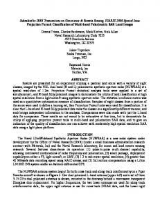
Figure 6 : The maximum sample size for the integer coecients for  19

m

2

The picture shows in the x-axis the sample size, in the y-axis the number of bits which are needed to represent the upper bound. The dotted lines are for  , the solid line for  for 625 (= 25  25), 2.500, 10.000 and 40.000 bins. We see if we have more than 600 datapoints and 2.500 bins our summation will probably cause an over ow for the coecients of  . In pictures of Figure 7 on the following page I compare the relative computing time of the density estimation using these integer coecients (see program A.5) against the time needed by the program with the binned version. Again the thick line indicates a ratio of 1:0. The thin solid lines are indicating ratios of 0:8, 0:6, ..., which means that the integer-coecient version is faster than the binned version. The dotted line indicates a ratio of 1:2. As we see I gain in fact some computational time, especially if I have only few observations (n < 500). The best result has the Logarithm-2 kernel. But I have also to look to the relative error for the estimated Friedman-Tukey index, which is shown in Figure 8. The results for the Uniform kernel are not shown because they are the same as in the binned version. As written above I run into trouble if I calculate the coecients of  . All pictures for the Quartic kernel show a big relative error "FT if I have more than 600 datapoints. For the Logarithm-2 kernel rises the question of the in uence of cutting the higher order terms. The graphic shows that the result is much more worse then for the Quartic kernel. In Figure 8 the thin solid line indicates a relative error of ..., 0.01%-, 0.1%. The lines cannot be distinguished. The thick line indicates an error of 1%. The dotted lines are indicating an error of 10% and 100% : 2

4

4

4

20

0.5 0.0 2.7

3.0

3.3

3.6

2.1

2.7

3.0 log10(n)

UNIFORM - QUARTIC

CIRCLE - QUARTIC

3.3

3.6

3.3

3.6

3.3

3.6

0.5 -2.0

-1.5

-1.0

-0.5

log10(h)

0.0

0.5 0.0 -0.5 -2.0

-1.5

-1.0

2.7

3.0

3.3

3.6

2.1

2.4

2.7

3.0

log10(n)

log10(n)

UNIFORM - LOG2

CIRCLE - LOG2

0.5 0.0 -1.0 -1.5 -2.0

-2.0

-1.5

-1.0

-0.5

log10(h)

0.0

0.5

1.0

2.4

1.0

2.1

-0.5

log10(h)

2.4

log10(n)

1.0

2.4

1.0

2.1

log10(h)

-0.5

log10(h)

-2.0

-1.5

-1.0

-0.5 -2.0

-1.5

-1.0

log10(h)

0.0

0.5

1.0

CIRCLE - UNIFORM

1.0

UNIFORM - UNIFORM

2.1

2.4

2.7

3.0

3.3

3.6

2.1

log10(n)

2.4

2.7

3.0 log10(n)

Figure 7 : Relative computational time for the Friedman-Tukey-index with binned data using integer-operations and oat-operations

21

0.5 0.0 2.7

3.0

3.3

3.6

2.1

2.4

2.7

3.0

log10(n)

log10(n)

CIRCLE - QUARTIC

CIRCLE - LOG2

3.3

3.6

3.3

3.6

0.5 0.0 -0.5 -1.0 -1.5 -2.0

-2.0

-1.5

-1.0

-0.5

log10(h)

0.0

0.5

1.0

2.4

1.0

2.1

log10(h)

-0.5

log10(h)

-2.0

-1.5

-1.0

-0.5 -2.0

-1.5

-1.0

log10(h)

0.0

0.5

1.0

UNIFORM - LOG2

1.0

UNIFORM - QUARTIC

2.1

2.4

2.7

3.0

3.3

3.6

2.1

2.4

log10(n)

2.7

3.0 log10(n)

Figure 8 : Relative error for the Friedman-Tukey-index using integer-operations for Quartic and Logarithm-2 kernel The result is disappointing for the computational time and the accuracy : The reason for this disappointing result is that I was forced to use a long integer. The computation for doing the calculations with long integers (4-byte) is faster than with oat-values, but slower than if I use 2-byte-integer. If we compare the inner loops for the density estimation with the Quartic kernel, we have to do on one side 4 oat-operations, on the other side 11 long-integer operations. For calculating the index function I used the routines in program A.6. Here there is some more potential for further optimization; for the Friedman-Tukey index and the Quartic kernel, we obtain then : n X 3 n ?2 I^FT (; ) = nh1  i i n ! X 3 = nh  ni ? 2 i 2

=1

2

=1

ni X

!

ri;j +

j =1 ni X j =1

2

!

ri;j + 2

ni X

!!!

ri;j

j =1 ni X j =1

4

!!

ri;j 4

;

where ni is the number of datapoints, which have distance ri;j < h to the datapoint Xi. I did not do further optimization, because I get even with the Quartic kernel over ows 22

for the density estimation. And summing up more distances ri;j will diminish the sample size where I can obtain correct results. 4

6 Conclusion It seems that replacing oat-operations by integer-operations is not very successful, except if the sample size is small (n < 250). First I have to ensure that I did not get a (long-) integer over ow. That means I am restricted, even with a moderate number of bins, in the sample size. The second point is that I have to restrict myself on some kernels. The in nite support and the lack of a summation formula expelled the Gaussian kernel. The diculties with the summation of dierent kernel-values forces me to expel the Triangle, Cosine and Logarithm-1 kernel. The bad results for the accuracy expelled the Logarithm2 kernel. For the XGOBI-program, for example, the Triweight kernel is used. I think the reason for this is that the partial derivatives after the projection vectors, which are used to speed up the maximization process, should be smooth enough. But I have to expel this kernel too, because with my binwidth (0:02) the sample size has to be less than 2, otherwise an long-integer- over ow can happen (50  2 ). This result is not too bad for the Quartic and Epanechnikov kernel, although we are restricted in the sample size. If we have a data set with more than 1000 datapoints, we can use other techniques than Project Pursuit methods for analysis. One reason to use projection Pursuit techniques was the "sparse of dimensionality" and sample sizes of 2000 or more are quite big. Even for small sample sizes the standard techniques like sorting and binning give some improvements in terms of computational time. 8

32

7 Extensions For small sample sizes (n < 500), the binning time plays also an important role. I replaced the binning-algorithm by the program A.7, and I lose the advantage that in one generated bin falls more than one datapoint. But for these sample sizes I do not expect that I have a lot of bins with more than one observation. In the following Table 4 I give the number of non-empty bins (on the average) for all the data sets : Observations Uniform Normal 100 98.0 93.3 200 191.9 172.6 500 451.5 353.7 1000 820.6 552.4 1367.5 774.0 2000 5000 2138.0 1072.0

Line Two Mass 94.6 94.6 179.0 178.1 382.4 375.5 612.4 605.2 859.5 866.0 1117.0 1211.0

Table 4 : Number of non-empty bins Total number of bins : 2500 23

Circle 96.8 186.2 416.2 705.0 1061.0 1457.0

As I mentioned in the introduction, we cannot capture two-dimensional structures very well by univariate projections. This is also true for trivariate structures, which cannot be caught by bivariate projections. In fact the binning technique can be extended to higher dimensions. But we run than in some serious problems :

 In general, if we do a density estimate, we have to be sure, that we are really esti-

mating the density. For higher dimensions it requires a big sample size to estimate the correct value. The following Table 5 from Silverman (1986) gives the required sample size for the multivariate normal density, such that the relative squared error E ('^(0) ? '(0)) ='(0) is less than 0:01. '^(0) is obtained by a kernel estimate : 2

2

Dimension Sample size 1 4 2 19 3 67 4 223 5 768 2790 6 7 10700 8 43700 9 187000 10 842000 Table 5 : Required sample size for estimating '(0) correct

 The second problem is, if I use program A.4 then I have to calculate kd (d is the dimension of the projection) kernel-values. If I would use the product kernel, it would be possible to store only k  d kernel-values and to calculate the product each time. But with these rotation-invariant kernels I would obtain (with k = 50 and d = 3) 125:000 kernel-evaluations. To store these values, because of speeding up the computational time, 1 MB of memory would be used. So this technique has to be modi ed. We can store only k + 1 knots Kn (0), Kn ( ),..., Kn (k ) and calculate each time the radius ri;j and "interpolate" then between the stored values of Kn to get a result for a kernel value. "Interpolate" here means replacing Kn (r) by a step function, or by a continuous function or by splines. This will clearly increase the computational time. I tried it out for the bivariate case and replaced K (r) by a step function with two dierent algorithms to nd the nearest knot (binary inserting and rounded squareroot). Both algorithms are 5 to 10 percent slower than program A.4, although I used only k kernel-values instead of k . This also reduces the accuracy. 2

2

Obviously the technique of reducing the oat-operations to integer-operations can be used in the one-dimensional case. 24

A C-Programs All the following programs use the knowledge that the data lie in [0; 1] : 2

A.1 For kernel-evaluation void qua (double *x, int n, double *y) /**********************************************************************/ /* Calculation for evaluating the comp. time for the Quartic kernel. */ /* It is assumed that the observations (x_1, y_1), ... (x_n, y_n) are */ /* stored in the array x. They are stored in the array x in the */ /* following way : */ /* */ /* x[0] = x_1 */ /* x[1] = x_2 */ /* ... */ /* x[n-1] = x_n */ /* x[n] = y_1 */ /* x[n+1] = y_2 */ /* ... */ /* x[2*n] = y_n */ /* */ /* First the distance to (0,0) and then QUA_2(r) is calculated. */ /**********************************************************************/ { double tmp, r; for (i=0; i