A Feature-Based Approach of Decision Tree

International Journal of

Geo-Information Article

A Feature-Based Approach of Decision Tree Classification to Map Time Series Urban Land Use and Land Cover with Landsat 5 TM and Landsat 8 OLI in a Coastal City, China Lizhong Hua 1 , Xinxin Zhang 1 , Xi Chen 2 , Kai Yin 3 and Lina Tang 4, * 1 2 3 4

*

College of Computer and Information Engineering, Xiamen University of Technology, 600 Ligong Road, Xiamen 361024, China; [email protected] (L.H.); [email protected] (X.Z.) School of Electronics and Information Engineering, Harbin Institute of Technology, 92 West Dazhi Street, Harbin 150001, China; [email protected] The Institute of Remote Sensing and Digital Earth, Chinese Academy of Sciences, 9 Dengzhuang South Road, Beijing 100101, China; [email protected] Key Lab of Urban Environment and Health, Institute of Urban Environment, Chinese Academy of Sciences, Xiamen 361021, China Correspondence: [email protected]; Tel.: +86-592-619-0681

Received: 13 August 2017; Accepted: 26 October 2017; Published: 31 October 2017

Abstract: Accurate mapping of temporal changes in urban land use and land cover (LULC) is important for monitoring urban expansion and changes in LULC, urban planning, environmental management, and environmental modeling. In this study, we present a feature-based approach of the decision tree classification (FBA-DTC) method for mapping LULC based on spectral and topographic information. Landsat 5 TM and Land 8 OLI images were employed, and the technique was applied to the coastal city of Xiamen, China. The method integrates multi-spectral features such as SAVI (soil adjustment vegetation index), NDWI (normalized water index), MNDBaI (modified normalized difference barren index), BI (brightness index), and WI (wetness index), with topographic features including DEM and slope. In addition, the new approach distinguishes between fallow land and cropland, and separates high-rise buildings from beaches and water bodies. Several of the FBA-DTC parameters (or rules) from 1997 to 2015 remained constant (i.e., DEM and slope), whereas others changed slightly. WI was negatively related to percent area of beach land, and BI was negatively related to percent area of arable land. The FBA-DTC method had an average user’s accuracy (UA) of 91.36% for built-up land, an average overall accuracy (OA) of 92.13%, and a Kappa coefficient (KC) of 0.90 for the period from 2003 to 2015, representing respective increases of 15.87%, 10.17%, and 0.13, compared with values calculated using maximum likelihood classification (MLC). Over the past 12 years, built-up land increased from 23.67% to 43.17% owing to occupation of coastal reclamation, arable land, and forest land. The FBA-DTC method presented here is a valuable technique for evaluating urban growth and changes in LULC classification for coastal cities. Keywords: decision tree classification; feature-based approach; urban land use and land cover; remote sensing; modeling; coastal city; Xiamen

1. Introduction Urbanization represents the territorial and socioeconomic progress of an area and is associated with the transformation of land use and land cover (LULC) types from undeveloped to developed [1]. Over recent decades, global urbanization has progressed rapidly [2]. In particular, coastal urban areas have experienced fast population explosion and dynamic economic growth. Knowledge of urban ISPRS Int. J. Geo-Inf. 2017, 6, 331; doi:10.3390/ijgi6110331

www.mdpi.com/journal/ijgi

ISPRS Int. J. Geo-Inf. 2017, 6, 331

2 of 18

LULC types and their areal distribution is essential for coping with a variety of environmental and socioeconomic issues [3,4]. Remote sensing can provide timely and detailed views of land cover, and thus is a useful approach for monitoring the growth and spatial distribution of urban areas [5]. Since the Landsat satellite was launched in the early 1970s, medium-resolution remote sensing imagery (15–30 m resolution) such as Thematic Mapper (TM), Enhanced Thematic Mapper Plus (ETM+), Landsat Operational Land Imager (OLI), Hyperion [6], and SPOT5 [7] images, and high spatial resolution imagery ( =P1 or Slope >= P2 Y

N

Hilly forest land

Non-hilly forest land NDWI >= P3 N

Y

Non-water body SAVI >= P4 N

Y

Vegetation BI >= P6

Non-vegetation MNDBaI(NDBaI) < P5

Y

N

Arable land

Y

Water body

Is it confused with built-up land?

Change detection by SAVI

N

Y

Forest land

Bare land

Non-bare land DEM >=P7 and WI < P8 N

Y

Built-up land

Beach land

Is it confused with the shadows of high-rise buildings ? Fallow cropland

Built-up land

Y

Change detection of built-up land and bare land

Beach land

Built-up land

Figure 3. Feature-based approach of decision tree classification constructed to extract urban LULC

Figure 3. Feature-based approach of decision tree classification constructed to extract urban LULC using Landsat 5 TM and Landsat 8 OLI data (see Figure 2 for key to abbreviations). using Landsat 5 TM and Landsat 8 OLI data (see Figure 2 for key to abbreviations).

3.2.1. Vegetation Index

3.2.1. Vegetation Index

Huete [38] proposed SAVI to extract vegetation based on a modified normalized difference Huete [38] proposed vegetation index (NDVI): SAVI to extract vegetation based on a modified normalized difference

vegetation index (NDVI):

SAVI = (ρNIR - ρRed )(1 + l) / (ρNIR + ρRed + l)

(3)

spectral of)(the respectively, for where ρNIR and ρRed are the SAV I = (ρreflectance 1 +red l )/and (ρ Nnear-infrared ) (3) N IR − ρ Red IR + ρ Red + l bands, the Landsat 5 TM and Landsat 8 OLI (TM/OLI); and l is a soil-adjusted factor with a value between 0 andρNIR 1. The default l value 0.5 canreflectance work well in situations [38]. Equation (3) produces valuesfor the where and ρRed are the of spectral of most the red and near-infrared bands, respectively,

Landsat 5 TM and Landsat 8 OLI (TM/OLI); and l is a soil-adjusted factor with a value between 0 and 1. The default l value of 0.5 can work well in most situations [38]. Equation (3) produces values in the range from −1 to 1, where positive values indicate vegetated areas and negative values signify non-vegetated surface features such as water, barren land, clouds, and snow.


7 of 18

in the range from −1 to 1, where positive values indicate vegetated areas and negative values signify 3.2.2. Water Index non-vegetated surface features such as water, barren land, clouds, and snow. McFeeters [39] presented NDWI to delineate open water features: 3.2.2. Water Index I= ρGreen − ρopen (ρGreenfeatures: + ρ N IR ) N IR ) /water McFeeters [39] presentedNDW NDWI to(delineate

(4)

NDWI = (ρGreen - ρof ) / (ρ ρNIR )near infrared bands for TM/OLI (4) where ρGreen and ρNIR are the spectral reflectance green NIRthe Green + and images, respectively. where ρGreen and ρNIR are the spectral reflectance of the green and near infrared bands for TM/OLI images, respectively. 3.2.3. Bare Land Index and Chen 3.2.3.Zhao Bare Land Index[40] proposed the Normalized Difference Bare Index (NDBaI) for bare land (i.e., land under development): Zhao and Chen [40] proposed the Normalized Difference Bare Index (NDBaI) for bare land (i.e., land under development): NDBaI = (dSWRI1 − d TIR )/(dSWRI1 + d TIR ) (5)

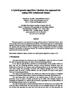
NDBaI = (dSWRI1 - dTIR ) / (dSWRI1 + dTIR ) (5) where dSWRI1 and dTIR are the raw digital numbers of the TM short-wave infrared (SWIR) 1 and thermal and dTIR are the raw digital numbers of the TM short-wave infrared (SWIR) 1 and where infrareddSWRI1 bands, respectively. thermal infrared However, webands, foundrespectively. NDBaI could not distinguish white tin roofs in urban villages from bare land. we urbanization, found NDBaIacould not of distinguish tin roofs in in urban villages from bare WithHowever, the dramatic vast area buildingswhite with bright roofs Xiamen has sprung up land. With the dramatic urbanization, a vast area of buildings with bright roofs in Xiamen has in recent years. Most of them may be posed by new attics built with white tin on top of the original sprung in recent years.the Most of them changes may be posed by tin new attics built with tintwo on urban top of houses. up Figure 4 showed significant of white roofs from 2003 to white 2014 in the original houses. showed the significant changes of white tin roofsnormalized from 2003 difference to 2014 in villages, Gaolin and Figure Wutong4 in Xiamen island. Therefore, we used a modified two urban(MNDBaI) villages, for Gaolin and in Wutong Xiamen island. Therefore, we exist. usedThe a modified bare index bare land cities inin which a number of the white roofs equation normalized difference bare index (MNDBaI) for bare land in cities in which a number of the white can be expressed as follows: roofs exist. The equation can be expressed as follows: MNDBaI = (ρ Red − ρ Blue )/(ρ Red + ρ Blue ) (6) MNDBaI = (ρRed - ρBlue ) / (ρRed + ρBlue ) (6) where and ρBlueare arethe thespectral spectralreflectance reflectanceofofred redand andblue bluebands bandsfor forTM/OLI TM/OLIimages, images,respectively. respectively. Red and ρBlue where ρρRed

Figure 4. Increase Increaseofofwhite whitetintin roofs in two urban villages, Gaolin (a) Wutong and Wutong of Xiamen Figure 4. roofs in two urban villages, Gaolin (a) and (b) of (b) Xiamen island, island, obtained from Google Earth from 2003 to 2014. obtained from Google Earth from 2003 to 2014.

3.2.4. Index 3.2.4. Brightness Brightness Index Index and and Wetness Wetness Index The defined by by Kauth and and Thomas [41] (1976), who The tasseled-cap tasseled-captransformation transformationwas wasoriginally originally defined Kauth Thomas [41] (1976), analyzed the spectra of wheat growth using using Landsat MSS. The transformation is executed by taking who analyzed the spectra of wheat growth Landsat MSS. The transformation is executed by linear combinations of the original or reflected image bands. In addition to Landsat Multispectral taking linear combinations of the original or reflected image bands. In addition to Landsat Multispectral Scanner transformation coefficients Landsat 5 5 TM, TM, ETM+, ETM+, IKONOS, Scanner MSS, MSS, transformation coefficients have have been been derived derived for for Landsat IKONOS, Landsat OLI, etc. etc. Landsat 88 OLI, The brightness index index (BI), (BI), the the first first tasseled-cap tasseled-cap band, band, corresponds corresponds to to the the overall overall brightness brightness of of The brightness an image. Cropland has aa higher higher brightness brightness value value than than forest forest land land (Figure (Figure 5). 5). an image. Cropland typically typically has


8 of 18


0.8

8 of 18

Forest land Water body Built-up areas Beach land

0.6

Mountain shadow Bare land Arable land

Surface reflectance

0.4 0.2 0 TM1

TM2

TM3

TM4

TM5

TM7

BI

WI

-0.2 -0.4

Band

Figure 5. Spectral profiles typicalland landuse use and and land in in thethe study areaarea in 2007. Figure 5. Spectral profiles ofof typical landcover covertypes types study in 2007.

Beaches are one of the most important land-use types in coastal cities, but it is difficult to

Beaches one of the built-up most important land-use types in coastal cities, but it is difficult to separate separate are beaches from land because of their similar spectral characteristics. The wetness beaches from built-up land because of their similar spectral characteristics. The wetness index index (WI), the third tasseled-cap band, is typically used as an index of “wetness” (e.g., soil or(WI), surface moisture). band, Compared with theused spectral characteristics of built-up(e.g., land,soil beaches have amoisture). high the third tasseled-cap is typically as an index of “wetness” or surface WI andwith low terrain. Thus, characteristics they can be distinguished from built-up landhave by combining image Compared the spectral of built-up land, beaches a high WI andanalysis low terrain. Tasseled cap transformation reflectance coefficients for TM andelevation OLI Thus,with theyelevation can be information. distinguished from built-up land by combining image analysis with images were cited from Crist [42] and Baig et al. [43], respectively: information. Tasseled cap transformation reflectance coefficients for TM and OLI images were cited 0.2043ρ + 0.4158ρ from Crist [42]BIand et al. respectively: (7) TM =Baig Blue [43], Green + 0.5524ρRed + 0.5741ρNIR + 0.3124ρSWIR1 + 0.2303ρSWIR2 WI

= 0.0315ρ

+ 0.2021ρ

+ 0.3102ρ

+ 0.1594ρ

- 0.6806ρ

- 0.6109ρ

Red SWIR1 SWIR2 BITM = TM 0.2043ρ Blue +Blue 0.4158ρGreenGreen + 0.5524ρ Red + 0.5741ρ N IRNIR+ 0.3124ρSW IR1 + 0.2303ρSW IR2

BIOLI = 0.3029ρBlue + 0.2786ρGreen + 0.4733ρRed + 0.5599ρ NIR + 0.508ρSWIR1 + 0.1872ρSWIR2

W ITM = 0.0315ρ Blue + 0.2021ρGreen + 0.3102ρ Red + 0.1594ρ N IR − 0.6806ρSW IR1 − 0.6109ρSW IR2

(8) (9)

(7) (8)

WIOLI = 0.1511ρBlue + 0.1973ρGreen + 0.3283ρ Red + 0.3407ρNIR - 0.7117ρSWIR1 - 0.4559ρSWIR2 (10) BIOLI = 0.3029ρ Blue + 0.2786ρGreen + 0.4733ρ Red + 0.5599ρ N IR + 0.508ρSW IR1 + 0.1872ρSW IR2 (9) where, ρGreen, ρBlue, ρRed, ρNIR, ρSWIR1, and ρSWIR2 are spectral reflectance values in the TM/OLI blue, green, W IOLIinfrared, = 0.1511ρshort-wave N IR − 0.7117ρ Green + 0.3283ρ SW IR1 − 0.4559ρ SW IR2bands, (10) Blue + 0.1973ρ Red + 0.3407ρ red, near infrared 1 (SWIR1), and short-wave infrared 2 (SWIR2) respectively; BITM and WITM represent the brightness index and wetness index for Landsat 5 TM, where, ρGreen , ρBlue , ρRed , ρNIR , ρSWIR1 , and ρSWIR2 are spectral reflectance values in the TM/OLI blue, respectively; and BIOLI and WIOLI represent the brightness index and wetness index for Landsat 8 green, red, near infrared, short-wave infrared 1 (SWIR1), and short-wave infrared 2 (SWIR2) bands, OLI, respectively.

respectively; BITM and WITM represent the brightness index and wetness index for Landsat 5 TM, respectively; and BIProcedure 3.2.5. FBA-DTC OLI and WIOLI represent the brightness index and wetness index for Landsat 8 OLI, respectively.

As shown in Figure 3, DEM and slope first are used to partition all pixels into two groups. The spectral characteristics of forests shadowed by mountains are similar to those of water bodies 3.2.5. FBA-DTC Procedure (Figure 5). However, certain forests typically grow above certain elevations or slopes, particularly in Xiamen. Therefore, topographic can be distinguish forests As shown in Figure 3, DEM andfeatures slope first areused usedto to partition mountain-shaded all pixels into two groups. from other classes such of as forests built-upshadowed land, water, other vegetation types. NDWIofiswater used bodies to The spectral characteristics byand mountains are similar to those distinguish water from other classes because water has a higher NDWI value than that of other classes. (Figure 5). However, certain forests typically grow above certain elevations or slopes, particularly in SAVI can be employed to separate vegetated areas (forest and cropland) from non-vegetated areas Xiamen. Therefore, topographic features can be used to distinguish mountain-shaded forests from (built-up land, bare land, and beaches). BI is helpful for distinguishing between forests and cropland other classes such as built-up land, water, and other vegetation types. NDWI is used to distinguish because cropland corresponds to a higher BI value compared with forests. water from other classes because has a land higher that of other classes. SAVI can The spectra of beach land water and built-up areNDWI similar value (Figurethan 5), but DEM and WI are helpful be employed to separate vegetated areas (forest and cropland) from non-vegetated areas (built-up for distinguishing between the two. Built-up land typically exists at higher elevation compared land, bare land, and beaches). BI isdue helpful forrapid distinguishing between forests and croplandgrowth, becausemore cropland with beaches. However, to the expansion of urban space and population corresponds tobeach a higher BIand value compared with forests. and more areas, even the surrounding sea, are being urbanized. Thus, WI is employed in combination with DEM to and distinguish and build-up The spectra of beach land built-upbetween land arebeaches similar (Figure 5), butland DEMwith andthe WI similar are helpful elevation, as beaches have a higher WI value than that of built-up land. for distinguishing between the two. Built-up land typically exists at higher elevation compared with

beaches. However, due to the rapid expansion of urban space and population growth, more and more beach areas, and even the surrounding sea, are being urbanized. Thus, WI is employed in combination


9 of 18

ISPRS Int. J. to Geo-Inf. 2017, 6, 331between beaches and build-up land with the similar elevation, as 9beaches of 18 with DEM distinguish have a higher WI value than that of built-up land. NDBaI or MNDBaI can be used to distinguish bare land from beaches and built-up land. NDBaI or MNDBaI can be used to distinguish bare land from beaches and built-up land. However, However, MNDBaI cannot be used to distinguish fallow land from bare land and NDBaI cannot be MNDBaI cannot be used to distinguish fallow land from bare land and NDBaI cannot be used to used to extract the buildings with white tin roofs. Thus, we used NDBaI for images from 2003 to extract the for buildings with2007 white tin roofs. Thus, we used NDBaI for images from 2003 to MNDBaI for MNDBaI those from to 2015. those from 2007 to 2015. During certain seasons, both fallow land and cropland (Figure 6) exist simultaneously, thereby During certain seasons, of both fallow cropland (FigureXiang’an 6) exist simultaneously, confounding the extraction these two land landand types. For example, district is one ofthereby the confounding theplanting extraction these bases two land types.because For example, Xiang’an districtclimate is one of thegreat biggest biggest carrot andofexport in China the district has suitable and carrot planting in China because thedistrict districtare hasusually suitableplanted climateduring and great sandy soil sandy soil for and the export growthbases of carrots. Carrots in the September for the growth of carrots. Carrots in the district are usually planted during September and October and October and harvested during May and June each year. Figure 6 shows distinctly different and harvested during May and June each year. Figure 6 shows response spectral response characteristics of lands in carrot farming on distinctly 28 Octoberdifferent (a) and spectral 8 January (b), respectively. In Figurein6a, yellow meanson very young leaves of 8carrots planted in October and pink 6a, characteristics of lands carrot farming 28 October (a) and January (b), respectively. In Figure meansmeans middle-aged leavesleaves of carrots planted in September. In Figure 6b, bright means mature yellow very young of carrots planted in October and pink meansred middle-aged leaves leaves of carrots that have grown for approximately 3 months. Furthermore, fallow land often of carrots planted in September. In Figure 6b, bright red means mature leaves of carrots that is have confused with built-up land. To solveFurthermore, this issue, it is critical to compare SAVI (viawith subtraction) grown for approximately 3 months. fallow land often is confused built-upfor land. two images from different seasons (i.e., one image in which either fallow land or cropland exist and To solve this issue, it is critical to compare SAVI (via subtraction) for two images from different seasons another in which both are present). (i.e., one image in which either fallow land or cropland exist and another in which both are present).

(b)

(a) A

(c) A

B

A B

B

Figure 6. Comparison of original images with undistinguishable fallow land and built-up land, and Figure 6. Comparison of original images with undistinguishable fallow land and built-up land, an arable land map: (a) original image in 2003; (b) original image in 2007; (c) arable land map and an arable land map: (a) original image in 2003; (b) original image in 2007; (c) arable land map extracted from feature-based approach of decision tree classification in 2003. Notes: A and B extracted from feature-based approach of decision tree classification in 2003. Notes: A and B represent represent built-up land and fallow land; CL and FL stand for cropland and fallow land. built-up land and fallow land; CL and FL stand for cropland and fallow land.

With the explosive population growth in Xiamen, high-rise buildings with 18 floors or more With the explosive population growth in the Xiamen, high-rise buildings 18 floors or of more have dramatically increased to accommodate increased population. Thewith spectral features suchdramatically buildings areincreased very similar to those of beaches and water, and cannot bespectral easily distinguished. have to accommodate the increased population. The features of such However, high-rise buildings often built over three years and may previous low-rise buildings are very similar to those ofare beaches and water, and cannot be arise easilyfrom distinguished. However, buildings or bare land. If bare land or built-up land from an early image (e.g., in 2007) is identified high-rise buildings often are built over three years and may arise from previous low-rise buildings or as land. a beach or water in subsequent (e.g.,(e.g., in 2015), indicates as that the latter bare If bare land orbody built-up land from animagery early image in 2007)this is identified a beach or water classification is likely incorrect. we indicates can detect thethe conversion of bare land to built-up body in subsequent imagery (e.g.,Therefore, in 2015), this that latter classification is likely incorrect. land by comparing different images. Therefore, we can detect the conversion of bare land to built-up land by comparing different images. 3.2.6.Calibration Calibrationof ofFBA-DTC FBA-DTC Parameters Parameters 3.2.6. Afterall allimages images were were corrected corrected for COST method, andand a dataset After for atmospheric atmosphericeffects effectsusing usingthe the COST method, a dataset for each image, including SAVI, NDWI, MNDBaI (or NDBaI), BI, and WI values, were produced for each image, including SAVI, NDWI, MNDBaI (or NDBaI), BI, and WI values, were produced (Equations (3)–(10)). (Equations (3)–(10)). We collected a minimum of 15 training sites for each LULC class in each Landsat scene We collected a minimum of 15 training sites for each LULC class in each Landsat scene processed processed by the COST model from 2003 to 2015. The training sites were redefined or added using by the COST model from 2003 to 2015. The training sites were redefined or added using Google Earth Google Earth (GE) images with the close acquisition dates as the original remotely sensed data. The (GE) images with the close acquisition dates as the original remotely sensed data. The size per training size per training site in the images ranged from 12 to 630 pixels. We could calculate a minimum site in the images ranged from 12 to 630 pixels. We could calculate a minimum pixel value in each pixel value in each image (the dataset, DEM, Slope, etc.) in training sites of its corresponding LULC image (the dataset, DEM,3,Slope, etc.) inThe training sites pixel of itsvalues corresponding LULC class class according to Figure respectively. minimum were the parameters in according Figure to3.Figure 3, respectively. The minimum pixel values were the parameters in Figure 3. For example, For example, the parameter P2 in Figure 3 was the minimum pixel value of NDWI image in


10 of 18

the parameter P2 in Figure 3 was the minimum pixel value of NDWI image in training sites for water body. Thus, we achieved an initial set of parameters of FBA-DTC. The parameters were further re-examined and modified based on LULC class accuracies wherever necessary till a satisfactory product was attained. 3.3. Accuracy Assessment Although ground data are required for accuracy assessments, such data are sometimes difficult and expensive to obtain, particularly historical data. Therefore, it is acceptable for high spatial resolution images and large-scale maps to be used as reference data [16]. In this study, independent ground samples were collected from GE images and used as reference data. GE provides free access to high-resolution satellite imagery. In addition to being used as “pictures” for visualization, GE has been recognized as a significant resource for ground-truth data [44], improving visual interpretation, and even classifying complex LULC types [45]. In order to obtain better reference data, the time stamps of the GE images we chose were as close as possible to those of the original images (2 March 2003, 5 December 2006, and 30 December 2014). It has been suggested that a minimum 50 samples (or pixels) of each class should be included in error analyses [16]. Here we used at least 60 samples for each class. For each scene, 800 samples were randomly selected using a stratified random sampling scheme and exported to GE for accuracy assessment. The classification results were evaluated based on a confusion matrix. Four validation metrics, kappa coefficient (KC), overall accuracy (OA), producer’s accuracy (PA), and user’s accuracy (UA), were determined from the matrix. UA is the inverse of the error of commission, i.e., UA = 1 − commission error, and PA is the inverse of the error of omission, i.e., PA = 1 − omission error. To evaluate the performance of the proposed FBA-DTC, a supervised maximum likelihood classification (MLC) method was conducted for the three Landsat images, resulting in three LULC maps. 4. Results and Discussion 4.1. FBA-DTC Results Extraction of LULC was carried out using DTC based on this dataset, DEM, and slope. Table 2 shows the parameters values derived from the dataset, DEM, and slope from 2003 to 2015. Some FBA-DTC parameters were constant, such as elevation and slope, and others only varied slightly. Built-up land was located in areas below 112 m elevation with a slope of 80% (Tables 3–5), and respectively. TheMLC. proposed achieved PA and most of the classes compared compared with MLC. The FBA-DTC method achieved UA and PA values of >80% (Tables 3–5), and produced (>90%) PA (orachieved very lowUA omission built-up land,3–5), water bodies, and with MLC.very The high FBA-DTC method and PA error) valuesfor of >80% (Tables and produced produced very high (>90%) PA (or very low omission error) for built-up land, water bodies, and foresthigh land(>90%) classification. lower (average from 2003 2015) bodies, for arable land thanland for very PA (or The veryUA lowwas omission error) for80% built-up land,towater and forest forest land classification. The UA was lower (average 80% from 2003 to 2015) for arable land than for other LULC types. In other somewhat higher occurred arable land classification. The UA was words, lower (average 80% fromerror 2003of tocommission 2015) for arable land for than for other other LULC types. In other words, somewhat higher error of commission occurred for arable land because someIn forest andsomewhat build-up land were mislabeled as arable land. This probably LULC types. otherland words, higher error of commission occurred for is arable land because because some forest land and build-up land were mislabeled as arable land. This is probably because arable land and forest land similar spectral Nevertheless, land and some forest landbarren and build-up landexhibited were mislabeled as arablevalues. land. This is probablyfallow because arable arable land and barren forest land exhibited similar spectral values. Nevertheless, fallow land and cropland were still distinguishable from built-up land (Figure 6c). Some build-up areas caused more land and barren forest land exhibited similar spectral values. Nevertheless, fallow land and cropland cropland were still distinguishable from built-up land (Figure 6c). Some build-up areas caused more confusion probably due from to mixed pixels consisting of Some roof tiles, concrete, vegetation, which were still distinguishable built-up land (Figure 6c). build-up areas and caused more confusion confusion probably due to mixed pixels consisting of roof tiles, concrete, and vegetation, which could give rise to confused spectra. could give rise to confused spectra.


12 of 18

probably due to mixed pixels consisting of roof tiles, concrete, and vegetation, which could give rise to confused spectra. Table 3. Accuracy assessment of feature-based approach of decision tree classification (FBA-DTC) and maximum likelihood classification for the 2015 image. Classified

Classified

Reference

Method

Data

FL

AL

WB

Beach

Data BUA

BL

Total

UA (%)

FBA-DTC

FL AL WB Beach BUA BL Total PA (%)

122 7 0 0 6 1 136 89.71

1 58 0 0 0 3 62 93.55

0 0 203 4 2 0 209 97.13

0 0 1 62 1 0 64 96.88

7 3 1 2 249 3 265 93.96

1 2 0 0 8 53 64 82.81

131 70 205 68 266 60 800

93.13 82.86 99.02 91.18 93.61 88.33

MLC


71 5 0 0 59 1 136 52.21

0 51 0 0 9 2 62 82.26

0 0 175 0 34 0 209 83.73

0 0 0 35 29 0 64 54.69

0 1 0 1 250 13 265 94.34

0 1 0 0 8 55 64 85.94

71 58 175 36 389 71

100.00 87.93 100.00 97.22 64.27 77.46

Note: FL, forest land; AL, arable land; WB, water body; BUA, built-up land; BL, bare land; PA, producer’s accuracy; UA, user’s accuracy.

Table 4. Accuracy assessment of feature-based approach of decision tree classification (FBA-DTC) and maximum likelihood classification for the 2007 image. (See Table 3 for key to abbreviations). Classified

Classified

Reference

Data

Method

Data

FL

AL

WB

Beach

BUA

BL

Total

UA (%)

FBA-DTC


131 8 0 0 6 1 146 89.73

2 60 0 0 2 1 65 92.31

0 0 202 20 4 0 226 89.38

0 0 0 73 1 0 74 98.65

1 3 0 1 215 0 220 97.73

0 3 0 0 8 58 69 84.06

134 74 202 94 236 60 800

97.76 81.08 100.00 77.66 91.10 96.67

MLC


117 6 0 0 22 1 146 80.14

7 55 0 0 2 1 65 84.62

0 0 196 5 24 1 226 86.73

0 0 5 62 7 0 74 83.78

1 2 0 0 212 5 220 96.36

0 2 0 0 14 53 69 76.81

125 65 201 67 281 61 800

93.60 84.62 97.51 92.54 75.44 86.89


13 of 18

Table 5. Accuracy assessment of feature-based approach of decision tree classification (FBA-DTC) and maximum likelihood classification for the 2003 image. Classified

Classified

Reference

Method

Data

FL

AL

WB

Beach

Data BUA

BL

Total

UA (%)

FBA-DTC


133 10 0 0 7 0 150 88.67

4 73 0 0 2 0 79 92.41

0 2 217 15 4 0 238 91.18

0 0 2 75 0 0 77 97.40

7 6 0 1 168 1 183 91.80

2 5 0 0 7 59 73 80.82

146 96 219 91 188 60 800

91.10 76.04 99.09 82.42 89.36 98.33

MLC


85 56 1 0 4 4 150 56.67

0 76 0 0 1 2 79 96.20

12 4 191 21 10 0 238 80.25

8 0 0 66 3 0 77 85.71

0 14 0 0 157 12 183 85.79

0 7 0 0 6 60 73 82.19

105 157 192 87 181 78 800

80.95 48.41 99.48 75.86 86.74 76.92

See Table 3 for key to abbreviations.

Table 6. Summary of major studies employing decision tree classification methods. Authors

Data Types

Methods

Pal and Mather [18]

Landsat 7 ETM+

Kandrika and Roy [25] Punia et al. [20] Qi et al. [26]

IRS-P6 AWiFS IRS-P6 AWiFS PolSAR

Boosted DTC MLC DTC (See-5) DTC (See-5) DTC-OOC MLC DTC MLC FBA-DTC MLC FBA-DTC MLC FBA-DTC MLC

Wang et al. [19] Hua et al. (this paper)

Landsat 5 TM Landsat 5 TM/2003 Landsat 5 TM/2007 Landsat 8 OLI/2015

LULC Classes

OA (%)

7 7 16 11 7 7 7 7 6 6

88.46 82.90 87.50 91.81 86.64 69.66 95.87 91.43 90.63 79.38 92.38 86.88 93.38 79.63

6

Increased OA (%)

Increased KC

0.87 0.80 0.87

5.56

0.07

0.84 0.65 0.88 0.74 0.90 0.83 0.92 0.73

16.98

0.19

4.44

-

11.25

0.14

5.50

0.07

13.75

0.19

KC

Note: DTC, decision tree classification; See-5, a commercially available decision tree algorithm; DTC-OOC, decision tree classification combined with object-oriented classification; feature-based approach of decision tree classification (FBA-DTC); MLC, maximum likelihood classification; OA, overall accuracy; KC, kappa coefficient.

Compared with FBA-DTC, MLC produced similar PA but much lower UA for built-up area classification, especially for the 2015 image (UA = 64.27%), for which large amount of forest land and water bodies were mislabeled as built-up land (Figure 9b). In contrast, the average UA for built-up land classified with the DLT method was 91.36% in 2003 and 2015, an increase of 15.87% compared with MLC. Compared to FBA-DTC, the UA for arable land derived from MLC decreased by 27.63% in 2003. Figure 7b shows that large areas of built-up land and forest land were mislabeled as arable land. MLC also displayed much lower UA for forest land classification in 2015 and 2003 compared with FBA-DTC. In addition, a large amount of forest land was not recognized (Figure 7b,f) with MLC. Our results were compared with those of previous studies that have employed DTC methods (Table 6). Wang et al. [19] prepared a LULC map of muddy tidal flat wetlands based on DTC and achieved an OA value of 95.84%, a 4.44% increase compared with MLC. Qi et al. [26] obtained a LULC map of the Panyu district in Guanzhou city, China using DTC combined with object-oriented classification (DTC-OOC) and RADRSAR-2 Polarimetric ASR (PolSAR) data. They estimated an OA of 86.64% and KC of 0.84, which corresponded to increases of 16.98% and 0.19 in comparison to respective values obtained with MLC. Pal and Mather [18] reported an OA of 88.46% and KC of 0.87 using

in 2003. Figure 7b shows that large areas of built-up land and forest land were mislabeled as arable land. MLC also displayed much lower UA for forest land classification in 2015 and 2003 compared with FBA-DTC. In addition, a large amount of forest land was not recognized (Figure 7b,f) with MLC. results were methods ISPRS Int.Our J. Geo-Inf. 2017, 6, 331compared with those of previous studies that have employed DTC 14 of 18 (Table 6). Wang et al. [19] prepared a LULC map of muddy tidal flat wetlands based on DTC and achieved an OA value of 95.84%, a 4.44% increase compared with MLC. Qi et al. [26] obtained a boosted anddistrict Roy [25] ancity, OA China of 87.50% and KCcombined of 0.87 with See-5 DTC and LULCDTC. map Kandrika of the Panyu in achieved Guanzhou using DTC with object-oriented IRS-P6 AWiFS data. Punia et al. [20] derived an OA of 91.81% using the same method as Kandrika andOA classification (DTC-OOC) and RADRSAR-2 Polarimetric ASR (PolSAR) data. They estimated an Roy Thus, theKC accuracy this study aretocomparable with thoseand of other of[25]. 86.64% and of 0.84,results whichfor corresponded increases of 16.98% 0.19 studies. in comparison to respective values obtained with MLC. Pal and Mather [18] reported an OA of 88.46% and KC of 0.87 4.3. Spatiotemporal LULC Changes using boosted DTC. Kandrika and Roy [25] achieved an OA of 87.50% and KC of 0.87 with See-5 Figures 9 and 10 show data. changes in LULC distributions and percentage thesame studymethod region as DTC and IRS-P6 AWiFS Punia et al. [20] derived an OAarea of 91.81% usinginthe from 2003 toand 2015. In[25]. order to remove the influence of this sea level area, water Kandrika Roy Thus, the accuracy results for studyon arebeach comparable with bodies those ofand other beaches were merged. Among all LULC types, built-up land increased the most, from 23.67% to studies. 43.17%, representing a 0.56-fold increase over the past 12 years. Urban land expansion was mainly 4.3. Spatiotemporal LULC Changes achieved by occupation of coastal reclamation, arable land, and forest land. Water bodies and beaches decreased the most, from 41.98% to 34.59%. One reason for the decrease in water bodies and beaches Figures 9 and 10 show changes in LULC distributions and area percentage in the study region may be related to a policy that was initiated to promote the conversion of Xiamen from an island city to from 2003 to 2015. In order to remove the influence of sea level on beach area, water bodies and a bay-like city [30]. Arable land showed the second largest decrease over the study period, from 9.13% beaches were merged. Among all LULC types, built-up land increased the most, from 23.67% to to 4.00%. Forest land remained basically stable from 2003 to 2015. For one thing, probably because it 43.17%, representing a 0.56-fold increase over the past 12 years. Urban land expansion was mainly was mostly located in hilly areas that were not suitable for urban land use. For other, forest land use achieved by occupation of coastal reclamation, arable land, and forest land. Water bodies and was limited by a policy concerning China’s national forest city in which the green coverage rate was beaches decreased the most, from 41.98% to 34.59%. One reason for the decrease in water bodies one of important evaluating indexes. and beaches may be related to a policy that was initiated to promote the conversion of Xiamen from (a)

(c)

(b)

(d)

Figure 9. Cont.


15 of 18


15 of 18

(f)

(e)

(f)

(e)

Figure 9. LULC classification results. (a) Feature-based approach of decision tree classification Figure 9. LULC classification results. (a) Feature-based approach of decision tree classification (FBA-DTC) applied to the image from 2015; (b) MLC applied to the image from 2015; (c) FBA-DTC (FBA-DTC) applied to the image from 2015; (b) MLC applied to the of image from 2015; (c) FBA-DTC Figure 9. LULC classification results. (a) Feature-based approach decision tree classification applied to the image from 2007; (d) MLC applied to the image from 2007; (e) FBA-DTC applied to the applied to the image from 2007; (d) MLC applied to the image from 2007; (e) FBA-DTC applied to the (FBA-DTC) applied to the image from 2015; (b) MLC applied to the image from 2015; (c) FBA-DTC image from 2003; (f) MLC applied to the image from 2003. image from (f)from MLC2007; applied to theapplied image from applied to the2003; image (d) MLC to the2003. image from 2007; (e) FBA-DTC applied to the image from 50 2003; (f) MLC applied to the image from 2003. 2003

Area percentage (%) Area percentage (%)

50 40

2003

2007

2007

2015

2015

40 30 30 20 20 10 10 0

0

Forest land Arable land Water body Beach land

Forest land Arable land Water body Beach land

Built-up Bare land land Built-up Bare land land

BW

BW

Figure 10. LULC changes in the study area from 2003 to 2015. Note: BW is the sum of beach land

and water bodies. Figure 10. LULC changes in the study area from 2003 to 2015. Note: BW is the sum of beach land and Figure 10. LULC changes in the study area from 2003 to 2015. Note: BW is the sum of beach land water bodies.

and water bodies.

5. Summary and Conclusions Monitoring the complex dynamics of cities requires consistent urban LULC maps spanning multiple time periods [3]. A variety of new techniques, in particular DTC, can help improve LULC classification and promote understanding of urban system dynamics. In this study, a FBA-DTC approach was proposed to extract urban LULC using Landsat 5 TM and Landsat 8 OLI data for a coastal city in southern China. The method’s suitability was assessed and the results were compared with those of an MLC-based approach and related studies. Urban LULC is diverse and complex, consisting of both continuous and discrete elements, which may pose problems such as mixed pixels and spectral variability in satellite image data [15]. The FBA-DTC method is based on spectral and topographic features of image data and specialized knowledge. Images used for classification were processed with COST atmospheric correction to avoid dramatically fluctuating spectral values. The advantages of multispectral features (SAVI, NDWI,


16 of 18

MNDBaI, BI, and WI) were combined with topographic features (DEM and Slope) and specialized knowledge to help avoid the spectral confusion to a large degree. The FBA-DTC method follows a set of clear classification rules that were constant or changed only slightly. Therefore, LULC can be rapidly and correctly classified over different time periods based on decision rules. We obtained reference data from GE images rather than ground data because collecting ground data can be expensive and sometimes unavailable. GE images are expected to provide ground truth data and improve data visualization, and can even automatically map LULC. The LULC classification accuracy of the FBA-DTC approach was higher than that of the MLC approach. FBA-DTC achieved an average OA of 92.13% and KC of 0.90, which were 10.17% and 0.13% higher than the MLC results, respectively. The FBA-DTC method greatly improved the classification accuracy of built-up land. The average UA for built-up land was 91.36%, which was 15.87% higher compared with the MLC results. The improved accuracy was likely due to FBA-DTC’s ability to separate bare land with light buildings from beach land and built-up land using MNDBaI and to distinguish beach land from built-up land using WI combined with elevation. Compared with other studies, the accuracy of the method presented here was satisfactory. Our research also explored temporal changes in LULC in the study area. Built-up land showed a 0.56-fold increase over the past 12 years. The rapid extension of built-up land was mainly due to occupation of coastal reclamation, arable land, and forest land. We developed a valuable method for quickly and objectively classifying urban LULC using parameters extracted from Landsat 5 TM and Landsat 8 OLI images with FBA-DTC. In the future, parameters should be further validated with more Landsat TM imagery and related data. It is essential to integrate other classification methods with image processing technology to improve classification accuracy. This study provides a reference for the LULC classification of coastal cities. Acknowledgments: This research was supported by the National Natural Science Foundation of China (No. 41471366), Young Scientists Fund of the National Natural Science Foundation of China under Grant (No. 41401475 and 41301455). Author Contributions: Lizhong Hua made substantial contributions to design, data processing and analysis. Lina Tang contributed to some conception of the study. Xinxin Zhang participated in revising it critically. Xi Chen contributed original Landsat images. Kai Yin was responsible for data cleaning. All authors had read and approved the final manuscript. Conflicts of Interest: The authors declare no conflict of interest.

References 1.

2. 3. 4. 5. 6.

7. 8.

Lu, L.L.; Guo, H.D.; Wang, C.Z.; Pesaresi, M.; Ehrlich, D. Monitoring bidecadal development of urban agglomeration with remote sensing images in the Jing-Jin-Tang area, China. J. Appl. Remote Sens. 2014, 8, 084592. [CrossRef] Grimm, N.B.; Faeth, S.H.; Golubiewski, N.E.; Wu, J.; Bai, X.M.; Briggs, J.M. Global Change and the Ecology of Cities. Science 2008, 319, 756–760. [CrossRef] [PubMed] Tong, X.H.; Xie, H.; Weng, Q.H. Urban land cover classification with airborne hyperspectral data: What features to use? IEEE J. Sel. Top. Appl. 2014, 7, 3998–4009. [CrossRef] Hu, T.; Yang, J.; Li, X.; Gong, P. Mapping Urban Land Use by Using Landsat Images and Open Social Data. Remote Sens. 2016, 8, 151. [CrossRef] Tian, Y.; Yin, K.; Lu, D.; Hua, L.Z.; Zhao, Q.J.; Wen, M.P. Examining Land Use and Land Cover Spatiotemporal Change and Driving Forces in Beijing from 1978 to 2010. Remote Sens. 2014, 6, 10593–10611. [CrossRef] Elatawneh, A.; Kalaitzidis, C.; Petropoulos, G.P.; Schneider, T. Evaluation of diverse classification approaches for land use/cover mapping in a Mediterranean region utilizing Hyperion data. Int. J. Digit. Earth 2014, 7, 194–216. [CrossRef] Davranche, A.; Lefebvre, G.; Poulin, B. Wetland monitoring using classification trees and SPOT-5 seasonal time series. Remote Sens. Environ. 2010, 114, 552–562. [CrossRef] Mathieu, R.; Aryal, J. Object-based classification of Ikonos imagery for mapping large-scale vegetation communities in urban areas. Sensors 2007, 7, 2860–2880. [CrossRef] [PubMed]


9. 10. 11.

12. 13. 14. 15.

16. 17. 18. 19. 20. 21. 22. 23.

24.

25. 26. 27. 28. 29.

30.

31. 32.

17 of 18

Lu, D.; Hetrick, S.; Moran, E. Land cover classification in a complex urban-rural landscape with quickbird imagery. Photogramm. Eng. Remote Sens. 2010, 76, 1159–1168. [CrossRef] Jawak, S.D.; Luis, A.J. Improved land cover mapping using high resolution multiangle 8-band WorldView-2 satellite remote sensing data. J. Appl. Remote Sens. 2013, 7, 073573. [CrossRef] Fauvel, M.; Benediktsson, J.A.; Chanussot, J.; Sveinsson, J.R. Spectral and spatial classification of hyperspectral data using SVMs and morphological profiles. IEEE Trans. Geosci. Remote Sens. 2008, 46, 3804–3814. [CrossRef] Guo, H.; Huang, Q.; Li, X.; Sun, Z.; Zhang, Y. Spatiotemporal analysis of urban environment based on the vegetation–impervious surface–soil model. J. Appl. Remote Sens. 2014, 8, 084597. [CrossRef] Yuan, H.; Van Der Wiele, C.F.; Khorram, S. An automated artificial neural network system for land use/land cover classification from Landsat TM imagery. Remote Sens. 2009, 1, 243–265. [CrossRef] Gopal, S.; Tang, X.J.; Phillips, N.; Nomack, M.; Pasquarella, V.; Pitts, J. Characterizing urban landscapes using fuzzy sets. Comput. Environ. Urban Syst. 2016, 57, 212–223. [CrossRef] Petropoulos, G.P.; Vadrevu, K.P.; Kalaitzidis, C. Spectral angle mapper and object-based classification combined with hyperspectral remote sensing imagery for obtaining land use/cover mapping in a Mediterranean region. Geocarto Int. 2013, 28, 114–129. [CrossRef] Lo, C.P.; Choi, J. A hybrid approach to urban land use/cover mapping using Landsat 7 Enhanced Thematic Mapper Plus (ETM+) images. Int. J. Remote Sens. 2004, 25, 2687–2700. [CrossRef] Wentz, E.A.; Nelson, D.; Rahman, A.; Stefanov, W.L.; Roy, S.S. Expert system classification of urban land use/cover for Delhi, India. Int. J. Remote Sens. 2008, 29, 4405–4427. [CrossRef] Pal, M.; Mather, P.M. An assessment of the effectiveness of decision tree methods for land cover classification. Remote Sens. Environ. 2003, 86, 554–565. [CrossRef] Wang, C.; Liu, H.Y.; Zhang, Y.; Li, Y.F. Classification of land-cover types in muddy tidal flat wetlands using remote sensing data. J. Appl. Remote Sens. 2013, 7, 073457. [CrossRef] Punia, M.; Joshi, P.K.; Porwal, M.C. Decision tree classification of land use land cover for Delhi, India using IRS-P6 AWiFS data. Expert Syst. Appl. 2011, 38, 5577–5583. [CrossRef] Baker, C.; Lawrence, R.; Montagne, C.; Patten, D. Mapping wetlands and riparian areas using Landsat ETM+ imagery and decision-tree-based models. Wetlands 2006, 26, 465–474. [CrossRef] Otukei, J.R.; Blaschke, T. Land cover change assessment using decision trees, support vector machines and maximum likelihood classification algorithms. Int. J. Appl. Earth Obs. Geoinf. 2010, 12, S27–S31. [CrossRef] Sesnie, S.E.; Gessler, P.E.; Finegan, B.; Thessler, S. Integrating Landsat TM and SRTM–DEM derived variables with decision trees for habitat classification and change detection in complex neotropical environments. Remote Sens. Environ. 2008, 112, 2145–2159. [CrossRef] Tooke, T.R.; Coops, N.C.; Goodwin, N.R.; Voogt, J.A. Extracting urban vegetation characteristics using spectral mixture analysis and decision tree classifications. Remote Sens. Environ. 2009, 113, 398–407. [CrossRef] Kandrika, S.; Roy, P.S. Land use land cover classification of Orissa using multi-temporal IRS-P6 awifs data: A decision tree approach. Int. J. Appl. Earth Obs. Geoinf. 2008, 10, 186–193. [CrossRef] Qi, Z.; Yeh, A.G.O.; Li, X.; Lin, Z. A novel algorithm for land use and land cover classification using RADARSAT-2 polarimetric SAR data. Remote Sens. Environ. 2012, 118, 21–39. [CrossRef] Powell, R.L.; Roberts, D.A.; Dennison, P.E.; Hess, L.L. Subpixel mapping of urban land cover using multiple endmember spectral mixture analysis: Manaus, Brazil. Remote Sens. Environ. 2007, 106, 253–267. [CrossRef] He, C.Y.; Shi, P.J.; Xie, D.Y.; Zhao, Y.Y. Improving the normalized difference built-up index to map urban built-up areas using a semiautomatic segmentation approach. Remote Sens. Lett. 2010, 1, 213–221. [CrossRef] Khatami, R.; Mountrakis, G.; Stehman, S.V. A meta-analysis of remote sensing research on supervised pixel-based land-cover image classification processes: General guidelines for practitioners and future research. Remote Sens. Environ. 2016, 177, 89–100. [CrossRef] Lin, T.; Xue, X.; Shi, L.; Gao, L. Urban spatial expansion and its impacts on island ecosystem services and landscape pattern: A case study of the island city of Xiamen, Southeast China. Ocean Coast. Manag. 2013, 81, 90–96. [CrossRef] Tang, L.N.; Zhao, Y.; Yin, K.; Zhao, J. City profile: Xiamen. Cities 2013, 31, 615–624. [CrossRef] Hua, L.Z.; Li, X.Q.; Tang, L.N.; Yin, K.; Zhao, Y. Spatio-temporal dynamic analysis of island-city landscape: A case study of Xiamen Island, China. Int. J. Sustain. Dev. World Ecol. 2010, 17, 273–278. [CrossRef]


33. 34. 35. 36. 37. 38. 39. 40.

41.

42. 43. 44.

45.

18 of 18

Hua, L.Z.; Tang, L.N.; Cui, S.H.; Yin, K. Simulating Urban Growth Using the SLEUTH Model in a Coastal Peri-Urban District in China. Sustainability 2014, 6, 3899–3914. [CrossRef] Hao, P.; Sliuzas, R.; Geertman, S. The development and redevelopment of urban villages in Shenzhen. Habitat Int. 2011, 35, 214–224. [CrossRef] Chavez, P.S. Image-based atmospheric corrections—Revisited and revised. Photogramm. Eng. Remote Sens. 1996, 62, 1025–1036. Wu, J.; Wang, D.; Bauer, M.E. Image-based atmospheric correction of QuickBird imagery of Minnesota cropland. Remote Sens. Environ. 2005, 99, 315–325. [CrossRef] Lu, D.; Mausel, P. Assessment of atmospheric correction methods applicable to Amazon basin LBA research. Int. J. Remote Sens. 2002, 23, 2651–2671. [CrossRef] Huete, A.R. A Soil-adjusted vegetation index (SAVI). Remote Sens. Environ. 1988, 25, 295–309. [CrossRef] McFeeters, S.K. The use of the Normalized Difference Water Index (NDWI) in the delineation of open water features. Int. J. Remote Sens. 1996, 17, 1425–1432. [CrossRef] Zhao, H.M.; Chen, X.L. Use of normalized difference bareness index in quickly mapping bare areas from TM/ETM+. In Proceedings of the 2005 IEEE International Geoscience and Remote Sensing Symposium, Seoul, Korea, 25–29 July 2005; pp. 1666–1668. Kauth, R.J.; Thomas, G.S. The tasseled cap—A graphic description of the spectral-temporal development of agricultural crops as seen by Landsat. In Proceedings of the Symposium on Machine Processing of Remotely Sensed Data, Purdue University, West Lafayette, IN, USA, 29 June–1 July 1976. Crist, E.P. A TM tasseled cap equivalent transformation for reflectance factor data. Remote Sens. Environ. 1985, 17, 301–306. [CrossRef] Baig, M.H.; Zhang, L.; Shuai, T.; Tong, Q. Derivation of a tasselled cap transformation based on Landsat 8 at-satellite reflectance. Remote Sens. Lett. 2014, 5, 423–431. [CrossRef] Biradar, C.M.; Thenkabail, P.S.; Noojipady, P.; Li, Y.; Dheeravath, V.; Turral, H.; Velpuri, M.; Gumma, M.K.; Gangalakunta, O.R.; Cai, X.L.; et al. A global map of rainfed cropland areas (GMRCA) at the end of last millennium using remote sensing. Int. J. Appl. Earth Obs. Geoinf. 2009, 11, 114–129. [CrossRef] Hu, Q.; Wu, W.; Xia, T.; Yu, Q.; Yang, P.; Li, Z.; Song, Q. Exploring the use of Google Earth imagery and object-based methods in land use/cover mapping. Remote Sens. 2013, 5, 6026–6042. [CrossRef] © 2017 by the authors. Licensee MDPI, Basel, Switzerland. This article is an open access article distributed under the terms and conditions of the Creative Commons Attribution (CC BY) license (http://creativecommons.org/licenses/by/4.0/).