A Framework for Re-Optimization of Repetitive Queries Feng Yu
Wen-Chi Hou
Cheng Luo
Qiang Zhu
Department of Computer Science Southern Illinois University Carbondale, IL, 62901
Department of Computer Science Southern Illinois University Carbondale, IL, 62901
Department of Computer Science Coppin State University Baltimore, MD
Department of Computer and Information Science University of Michigan Dearborn, MI 48128
[email protected]
[email protected]
ABSTRACT Optimizing executions of queries is the ultimate goal of the query optimizer. Unfortunately, due to the complexities of queries, accuracy of statistics, validities of assumptions, etc., query optimizers often cannot find the best execution plans in their search spaces, conveniently called the optimal plans, for the queries. In this paper, we develop a comprehensive framework for re-optimization of a large and useful set of queries, called repetitive queries. Repetitive queries refer to those queries that are likely to be used repeatedly or frequently in the future. They are usually stored in the database for convenient reuses for the long term. They deserve more optimization efforts than ordinary ad hoc queries. In this research, we identify statistics, called sufficient statistics, that are sufficient to compute the exact intermediate results of all plans of a query. The finding of the sufficient statistics makes it entirely possible for an optimizer to find the truly best plan in its search space for a query. We present two innovative techniques to conduct re-optimization, an eager and a lazy re-optimization. The eager approach gathers all the sufficient statistics at once and generates the best plan. The lazy approach gathers only the statistics that are needed to correct large estimation errors found in the plan and generates a revised plan. We further adapt the two basic techniques to constantly changing database environments by continuously monitoring and revising the plans, called adaptive re-optimization. The adaptive reoptimization is devised to detect and remedy potential suboptimality in the plans in a timely manner for the entire lifetime of the query. We have also designed an approximate re-optimization method that provides an efficient and effective alternative to refining query execution plans. Our work realizes the promise made by the query optimizers, namely, executing queries in the optimal fashions, at least for the repetitive queries.
1. INTRODUCTION Query optimization aims to find the most efficient plans for the executions of queries. It has been a central research topic of databases for the last few decades [9, 10, 12, 13, 20, 21, 23, 25, etc.]. A query optimizer generally uses statistics on databases [15,
Permission to copy without fee all or part of this material is granted provided that the copies are not made or distributed for direct commercial advantage, the VLDB copyright notice and the title of the publication and its date appear, and notice is given that copying is by permission of the Very Large Database Endowment. To copy otherwise, or to republish, to post on servers or to redistribute to lists, requires a fee and/or special permissions from the publisher, ACM. VLDB ’10, September 13-17, 2010, Singapore. Copyright 2010 VLDB Endowment, ACM 000-0-00000-000-0/00/00.
[email protected]
[email protected] 18, etc.] and assumptions about attribute values [4, 20] to estimate the cost of alternative plans and selects the best for executions. It is important for an optimizer to find the most efficient plans because studies [4, 14] have shown that executions with suboptimal plans can be orders of magnitude slower than with the optimal ones. Unfortunately, due to the sufficiency of statistics stored in the database catalog and the validity of assumptions made, query optimizers often cannot find the plan that is truly the best in their search spaces for the queries. Thus, some database systems, like Sybase and Oracle, allow users to force the join orders; some, e.g., Sybase, even allow users to explicitly edit the plans [19]. Unfortunately, such measures cannot guarantee success and can also be cumbersome and slow for complex queries. Clearly, there is a tremendous need for a mechanism that can automatically refine the execution plans of queries. Query re-optimization aims to refine the execution plans of queries. It can have a tremendous impact on the performance of systems. Unfortunately, there hasn't been much work on this subject yet. In the literature, some [2, 11, 14, 16] have focused on refining execution plans of ongoing queries on-the-fly, while others [3, 22] focused on refining cost estimation of future queries using statistics collected in the previous executions. In this paper, we are interested in refining cost estimation and execution plans of future queries, similar to the latter. Stillger et al. [22] collected cardinality information from queries and used it to adjust the cost estimation of future queries. Unfortunately, statistics, like cardinalities and selectivities, obtained from one plan may not be sufficient for estimation of another plan because as the orders of joins change, the inputs of the joins and the outputs thereof are all changed; they certainly are not sufficient for estimation of different queries. The situation is further exacerbated by adding other operators, such as selects, projects, unions, and differences, to the queries. It can require prohibitively large amounts of statistics, if ever possible, to compute the intermediate results’ sizes for all possible plans of all queries. Therefore, in this research, we set a more realistic goal by restricting ourselves to optimizing a subset, but a large and useful subset, of queries, called repetitive queries. Many queries are posted only once or a few times before discarded totally, hereby called ad hoc queries. There are also many useful queries, such as those used for generating periodic reports, performing routine maintenances, summarizing and grouping data for analysis, etc., that are run frequently, periodically, or repeatedly, hereby called repetitive queries. They are often stored in the database for convenient re-uses for the long term. As new queries are continually being developed, useful ones are also continually being added to the system for repetitive uses 1
in the future. Usually, the longer the database has been in production, the larger the number of repetitive queries is in the database. They can constitute a large portion of the daily activities. Any sub-optimality in the execution plans of repetitive queries could mean repetitive and continued wastes of system resources and time in the future. Repetitive queries have profound impacts on the performance of systems and deserve more optimization efforts than ad hoc queries. With a successful reoptimization mechanism implemented, a large portion of the daily tasks can be executed in the optimal fashions, fulfilling the promise that has long been made by the query optimizer, at least, for a large and useful set of queries.
identify statistics that are sufficient to compute the intermediate results of all plans of a query. In Section 5, we present different ways to collect the sufficient statistics. In Section 6, we propose several innovative ways to conduct re-optimization. Section 7 is the conclusions and future work.
2. LITERATURE SURVEY The work in query re-optimization can be classified into two categories: (1) re-optimizations of ongoing queries and (2) reoptimization of future queries. Our work falls into the second category. Most re-optimization work [2, 11, 14] belongs to the first category. Kabra et al. [11] collected statistics during the execution of a query and used them to optimize the rest of the execution by either changing the execution plan or improving the resource allocations. Heuristics were used to determine if the benefits of reoptimization outweighed the overheads. Markl et al [14] computed the validity range of each plan. When the actual result falls outside the validity range, a re-optimization is triggered. Intermediate results are saved for potential re-uses in the new join order. Instead of computing a point estimate of the cardinality of an operator, Babu, et al [2] used interval estimates (or bounding boxes) to account for the uncertainty of the estimation. Within the bounding box, they selected robust and switchable plans that avoid re-optimization and loss of pipelined work done earlier.
In this research, we present a comprehensive framework for reoptimization of repetitive queries. Knowing the shortcomings of using cardinalities and selectivities in estimation of the sizes of intermediate results, in this research, we identify statistics, called sufficient statistics, that are sufficient to compute the sizes of intermediate results of all plans (defined in Section 3.1) of a query. We consider queries with select, bag/set project, Cartesian product, bag/set union, and bag/set difference operations in the forms of linear as well as bushy trees [10, 19]. The relations can be bags as well as sets of tuples. The sufficient statistics can be gathered either on-line at runtime or off-line in spare time. The gathered statistics can be used by the (existing) query optimizer to find the best plan in its search space, conveniently called the optimal plan here. In fact, the sufficient statistics are sufficient to find the best plan of a query from a much larger solution space than that an ordinary optimizer searches.
Other remotely related work in the first category includes Avnur's Eddies [1], Urhan's query scrambling [24] and Ng's Conquest [16]. In a constantly fluctuating environment, tuples in Eddies are shipped to an operator (e.g., a join) for processing and then sent back to the system for further processing [1]. It re-optimizes the execution by allowing tuples to flow through operators in different orders to adapt to the system resource and workload conditions. Urhan, et al. [24] modified the execution plans when delays were encountered in a wide-area network environment. The system hides the delays by performing other useful work. Ng et al. [16] collected statistics at runtime and modified the execution plans based on the availability of system resources in an extensible and distributed environment.
We present two innovative methods to conduct query reoptimization, an eager and a lazy approach. The eager approach gathers all the sufficient statistics at once and derives the optimal plans. The lazy re-optimization gathers only the statistics that are needed to correct large cardinality estimation errors found in the plan and generates a revised plan; it may take a few cycles to attain the optimal plan in this approach. We adapt the two basic re-optimization techniques to constantly changing database environments by continuously monitoring the executions and revising the plans, called the adaptive re-optimization. With the adaptive re-optimization, sub-optimality can be detected and remedied timely to guarantee the optimality of plans for the entire lifetime of the query without human intervention. We have also devised an approximate re-optimization method to simplify the computations of intermediate results' sizes, however, at the price of accuracy. The approximate re-optimization presents an efficient and effective alternative to refining execution plans.
[3, 22] fall in the second category. Stillger et al. [22] collected cardinalities of operators and used them to adjust the selectivity estimation of future queries. This method could work well if the query bears a strong resemblance to the previous ones. Chaudhuri, et al. [3] used distinct page count, as opposed to the cardinality, as the cost measure for an operator. The page count accounts for the clustering effect of data on the disks, reflecting the computation cost or time in a more direct way.
Our work distinguishes itself from others in the area of query reoptimization. We present a comprehensive solution to the reoptimization of repetitive queries. We cover a large class of queries that includes the select, project, Cartesian product, union and difference operations on bags and sets of tuples in the forms of linear and bushy trees. The identification of the sufficient statistics makes it entirely possible to compute the exact intermediate results of all plans of a query and hence the reoptimization. We propose several innovative ways to conduct reoptimizations, realizing the ultimate goal of query optimization for repetitive queries.
3. RE-OPTIMIZATION FRAMEWORK First, we briefly review some background knowledge and then describe the re-optimization framework.
3.1 Background and Terminology In the formal relational model, relations are set of tuples; duplicates are not allowed in either the relations or query results. But, in commercial DBMSs, relations are often implemented as bags, rather than sets, because retaining duplicates can be more efficient for operators like projects and unions, and sometimes necessary for computing aggregate functions [6]. To convert a bag into a set, the keyword "DISTINCT" can be specified in the SELECT statement of SQL. Here, we allow a relation to be a set or a bag of tuples. We shall call the data model that allow
The rest of the paper is organized as follows. In Section 2, we briefly review papers related to the query re-optimization. In Section 3, we propose a re-optimization framework and give a functional overview of each component of it. In Section 4, we 2
interfering with the executions of queries. Section 5 has more details on these approaches.
relations and query results to be bags as the bag model, as opposed to the traditional relational model, which is a set model.
Query
In this paper, we limit ourselves to queries that can be expressed by the five basic operators – select, (set/bag) project, Cartesian product, (set/bag) union and (set/bag) difference. The set and bag project refer to the projections that eliminate and retain duplicates produced in the project operations, respectively. We will make such distinction only when necessary. We shall use a (theta-)join and a Cartesian-product followed by a selection with conditions specifying some (theta-)join conditions, interchangeably.
Execution Plan
Query Processing Online Statistics Gathering
We assume there are mechanisms in the system that can determine whether a query is a repetitive query or not. For example, the system can designate a stored query that has been run more than a certain number n ( 0 of times as a repetitive query; or simply allows a user to designate a query as a repetitive query as (s)he likes.
Result
In this paper, we use a plan, a query plan, and an execution plan, interchangeably. They all refer to the logical execution plan of a query, concerning about the execution orders of the operators in the queries.
Re-optimizer Adaptive
Approximate
Eager
Lazy
Revised Plans Statistics
Offline Statistics Gathering
Query Optimizer
An Optimal or Revised Plan
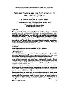
Figure 3.1 Re-optimization Architecture
The re-optimizer supplies the statistics gathered to the query optimizer to generate the optimal or a revised plan. Dependent upon the amounts of statistics supplied to the optimizer, the re-optimization can be conducted either in an eager or a lazy fashion. The eager re-optimization refers to the situations where all the sufficient statistics of a query are provided to the optimizer at once to generate the optimal plan. As for the lazy re-optimization, only selected statistics that are likely to correct large estimation errors found in the plan are gathered and provided to the optimizer to generate a revised plan. It may take a few cycles to arrive at the optimal plan. The optimal or revised plan is stored in the system for subsequent executions of the query.
To find the optimal execution plan for a query, accurate cost estimates of alternative plans must be computed, which are mainly determined by the intermediate results’ cardinalities (or sizes). We intend to identify statistics, called sufficient statistics, that are sufficient to compute the exact intermediate results' data distributions (and thus surely the cardinalities too) of all plans of a query. Here, all plans of a query refer to all alternative plans that can be derived by applying the commonly used relational algebraic laws [5, 6, etc] and optimization heuristics - pushing selections and projections as far down the trees as possible. The sufficient statistics, to be discussed shortly in Section 4, are in fact the joint frequency distributions of the "deciding" attributes of the operand relations.
The adaptive re-optimization is devised to maintain the optimality of the plans throughout the lifetime of the query. By continuously monitoring the executions and modifying the plans, if necessary, optimality can be maintained even though the underlying database has undergone substantial changes. The adaptive re-optimization can be accomplished by using either the eager or the lazy reoptimization method. The approximate re-optimization is designed to reduce the cost of computing (the frequency distributions of) the intermediate results, however at the price of accuracy. Section 6 has detailed discussions on these reoptimization methods.
As the number of relations involved in a query increases, the number of possible join orders increases exponentially. It has been shown that it is an NP problem to find the absolute optimal join order for a query [8, 17]. Thus, a query optimizer usually searches only a small portion of the possible join order space. Consequently, an optimal plan here refers to the best plan that can be found in the optimizer’s search space (a relative term), although the sufficient statistics discussed here are sufficient to find the best plan of a much larger solution space than that an ordinary query optimizer searches.
Since the re-optimization is mainly an off-line process, it can afford to use more time and resources to search for a better plan. Therefore, it may be worth employing a more sophisticated query optimizer that searches a larger solution space. Note that the proposed sufficient statistics are sufficient for computing the exact intermediate results’ sizes of all plans of a query derived by using the commonly used algebraic laws and optimization heuristics.
3.2 Architecture In Figure 3.1, we outline the re-optimization framework with the solid lines and arrows highlighting the new components and paths added to the database system while the dotted lines the existing components and paths. Note that we do not intend to modify the existing query optimizers, but just to provide them with sufficient statistics to find the execution plans that are truly the best in their search spaces.
4. SUFFICIENT STATISTICS Query optimizers employ strategies, such as the relational algebraic laws (for sets and bags) and heuristics, to generate alternative plans. Each plan generates its own set of intermediate results and may require a different set of statistics to compute their sizes. In order to find the statistics that are sufficient to compute the intermediate results’ sizes of all plans of a query, we need to know the strategies applied and the plans generated.
When a repetitive query is being executed, statistics can be collected, as indicated by the on-line statistics gathering box in the figure. One can also gather the statistics off-line whenever it is convenient, especially in spare time, as indicated by the off-line statistical gathering box. The on-line approach takes advantage of the query evaluation to gather readily available statistics while the off-line approach gathers the sufficient statistics without 3
Query Optimization
shall allow the optimizers to explore linear trees (e.g., left- and right-deep trees) as well as bushy trees. However, for simplicity of illustration, all examples here use left-deep trees; but the results should apply to bushy trees too.
4.1 Optimization Strategies and Assumptions In order for this framework to be as general as possible, we assume only those common strategies and heuristics used by most, if not all, of the optimizers are applied here. In the following, we review these strategies and heuristics that could affect the plans generated.
Let us emphasize again that all plans of a query refer to all alternative plans generated by using the commonly used algebraic laws (for bags and sets) and heuristics mentioned above. They should cover a much larger solution space than that an ordinary query optimizer searches.
Algebraic Laws. We assume the commonly used algebraic laws [5, 6, etc], such as the commutative and associative laws for joins, Cartesian product, and unions, and the laws for pushing of selections and projections, are used to generate alternative plans. Although there are some other rules applicable, such as the distributive law of joins over set and bag unions and difference, i.e., / / , and rules in the set theory, e.g., , we shall not assume the applications of them as they generally are not used by the optimizers and bring no benefit to the query evaluation.
4.2 Common Properties of Execution Trees We wish to identify some useful properties of the plans generated. In the following, we use an example to illustrate our observations on the execution plans of queries. Consider a university database with three relations: (teaching) Assignment(course_id, tname, dept), Books (book_id, title, publisher), and CoursesText(course_id, book_id), with their keys underlined. We assume a course can use more than one textbook. Consider the query: Print the titles of the books published by “PH” and used in the courses taught by teachers in the CS department. Figure 4.1 show two alternative plans of the query in which selections and projections have been pushed down.
Pushing Selections. Select conditions are normally expressed in … , or converted into the conjunctive normal form, where ’s, 1 , are the selection conditions. Selections tend to reduce the sizes of relations dramatically. Pushing selections down has been one of the most powerful tools used by the query optimizers. Therefore, we shall assume all query optimizers apply this heuristic: selections are pushed as far down the tree as possible. It is mentioned [6] that when views/sub-queries are used in the queries as operands, selections should first be pushed up and then pushed down to exploit the full benefit of pushing down selections. Such an enhancement fits right with our framework. Pushing Projections. Pushing projections as far down the tree as possible eliminates unused attributes at the earliest possible time and can be very beneficial to the query processing. Although pushing projections can add more projections down the tree, projections can be executed with succeeding selections and binary operations together without incurring extra cost. Therefore, we shall assume the commonly used pushing projections heuristics is applied here.
Figure 4.1 Execution Plans In the figure, we have used, for simplicity, A for Assignment, B for Books, and C for CourseText. In addition, a Cartesian-product preceded by a selection that specifies a natural join condition has been replaced by a natural join operator and its join attribute. The two plans have different join orders.
Normally, projections are pushed down after selections and they would not be pushed below the selections that directly apply to operand relations [4, 5]. If the pushing of a projection must stop at a certain operation, new pushes ought to be initiated at its operands. For example, the pushing of a bag/set projection must stop at the difference operation because ; new pushes should be initiated at and if and themselves have projections. In addition, the set projection cannot be pushed through the bag union while the bag projection cannot be pushed through the set union; new pushes of projections should be initiated at their operands too.
Example 1. In Figure 4.1 (a) and (b), operand relations A, B, and C each are preceded by the same select operations in both plans. That is, in both plans, A is preceded by " " , (i.e. ), B by ), " " " " (i.e. " " and C by no selection (or a selection with a predicate that every tuple satisfies). □
Definition. Initial Projection. An initial projection refers to a projection in a plan from which a new and independent push of projection is initiated.
Here, we call an operand relation R and its preceding selection, probably none, the select-modified relation of R, denoted by R’.
Consider Figure 4.1. The topmost that produces the final result is the only initial projection in the tree because there is no operator, like difference or bag/set union, blocking the pushes of projections.
Definition. Select-modified relation. Let R be an operand relation of a query. After selections have been pushed as far down the tree as possible, the select-modified relation of R, denoted by R’, refers to R and its immediate preceding selection, if any, in the tree. If R has no selection preceding it, R itself is the selectmodified relation of R. □
Linear and Bush Trees. While most optimizers explore linear execution trees, some explore bushy trees [19]. Therefore, we 4
The reason that each operand relation is preceded by the same select conditions in all plans is that selection conditions on individual relations will eventually all be pushed down to respective relations, no matter what the join orders are – thanks to the heuristic of pushing down selections and the algebraic laws. Lemma 1 gives a formal proof of this property.
Let us consider the five basic operators - select, project, Cartesian product, union, and difference, that may appear in the queries. We wish to identify the attributes that are used in these operators to decide on the outputs. Selection. Selection conditions are expressed in the conjunctive … . All conditions , 1 normal form as , can be pushed down, except those specifying the -)join conditions, e.g., . . , where , , , , , and those referencing attributes of more than one relation and connected by the “or” connectives, e.g., . 5 . 40. Obviously, the attributes specified in such “non-pusheddown” conditions, like . , . , . , and . , would be used to decide on the outputs and thus should be included in the bases of respective frequency distributions’ domains.
LEMMA 1. Each operand relation is preceded by the same selection conditions, if any, in all plans of the query. and be two plans in Proof: Prove by contradiction. Let which selections have been pushed as far down the trees as possible. Assume relation R is preceded by a selection condition in plan , but not in . Then, by the assumption of conjunctive selection conditions, must be a condition on attributes of only . Since no selection can be lost or new selection conditions be created in the process of pushing, Fi must appear somewhere in the tree for . However, according to the relational algebraic laws for sets and bags, the selection condition can pass through any select, Cartesian-product, projection, union and difference operators, until reaching in , regardless of the data model, set or bag model, and type of trees, linear or bushy. Thus, the condition must have not been pushed down as far as possible in – a contradiction.□
Projection. We differentiate a bag projection from a set projection here. In the bag projection, the project attributes are used only to remove unwanted attributes; every input tuple would become an output. Therefore, no projection attribute needs to be added to the basis of any frequency distribution’s domain. As for the set projection, the project attributes are used to determine and remove duplicacy and thus should be included into the bases of appropriate frequency distributions' domains. Cartesian-product. The Cartesian-product does not use any attribute to decide on the outputs. Consequently, no attribute needs to be added to the basis of any frequency distribution’s domain.
From the above discussions, we see that each operand relation is first modified by the same selection operations in all plans of the query (Lemma 1) and then participate in the rest of the operations. Therefore, we can consider the select-modified relations, or simply called the modified relations, as the immediate inputs to the queries.
4.3 Sufficient Statistics Intermediate Results
for
Union. The bag union operator generates output tuples by merging the input tuples without consulting any attribute. So, no attribute needs to be added to the basis of any frequency distribution’s domain. As for the set union operation, the key attribute values of the tuples are used to determine duplicacy and the outputs. Therefore, the key attributes of the operand relations of the union, which may be results of sub-queries, must be added to the bases of the respective frequency distributions’ domains. Here, the key attributes refer to the key attributes of the inputs of the union operation, if they have; otherwise, the entire set of attributes is regarded as the key.
Computing
As just mentioned that modified relations can be viewed as the immediate inputs to the queries, our idea is to keep, for each modified relation, a joint frequency distribution of its "deciding" attributes such that the frequency distributions (and surely the sizes) of the outputs of all operators in all plans of the query can be derived. The frequency distribution of a modified relation can be viewed as an n-dimensional histogram, where n is the number of the "deciding" attributes of the modified relation. The “deciding” attributes form the basis of the joint frequency distribution’s domain of the modified relation. Hereafter, we shall use the deciding attributes and basis attributes interchangeably. The histogram records the numbers of tuples in the modified relation that have the respective combinations of basis attribute values. In this subsection, we determine what attributes of a modified relation constitute the basis attributes.
Difference. In both the bag and set difference operations, the key attribute values of the input tuples must be compared to determine the output tuples. Therefore, we shall include the key attributes of the operands in the bases of the respective frequency distributions’ domains.
4.3.1 Basis of Frequency Distribution’s Domain
Let "mr" be a variable representing the modified relation of an operand relation of the query. Let attr(mr) be the set of attributes of the modified relation "mr", and basis(mr) be the set of basis attributes for "mr". We assume the highest node representing the modified relation has been marked as a modified relation. For example, for the select-modified relation , we " " assmue the node " " has been marked as a modified relation.
We summarize the above discussions on identifying the basis attributes into the following algorithm. The algorithm performs a post-order traversal of the execution tree and uses "bases" to store all basis attributes. At the end, at the root node, it constructs the bases for individual modified relations from the "bases".
An operator usually determines if an output tuple should be generated by examining the values of some designated attributes of the input tuples. For instance, a select operator checks the values of the attributes specified in the selection conditions to determine the outputs. Therefore, to construct the output frequency distribution of the result of an operator, one must incorporate these deciding attributes (or basis attributes) into the bases of its input frequency distributions’ domains. In the following, we discuss how to identify the basis attributes from each operator.
Algorithm Dist_Domain_Bases (node, bases) { 5
Example 3. SELECT DISTINCT statements. Consider the plans in Figure 4.1(a) and (b) again and let the projections in the trees now be the set projections. For modified relation A’, basis(A’) = {course_id} because course_id is a join attribute and also an attribute of the set projection For ’ , _ . basis{B’}={book_id, title} because book_id is both a join and a set project attribute while title appears in a set projection. Notice that title was not included in basis{B’} in Example 2 because the projections were bag projections. For ’, basis(C’)={course_id, book_id} because course_id is a join attribute and book_id is both a join and a set project attribute. □
if (node is not a modified relation) { for (each childnode of node ) Dist-Domain_Bases (childnode, bases); switch (type of node) { Case root: for (each modified relation mr) { basis(mr)=bases attr(mr); if (basis(mr)= basis(mr)={count}; } Case select: = {attributes in the selection condition}; Case set projection: = {attributes on the projection list }; Case difference: = {key attributes in the operand relations}; Case set union: = {key attributes in the operand relations}; } }
Again, in Example 3, one can use either the plan in Figure 4.1(a) or (b) to find the bases of the frequency distributions’ domains and the results are the same. The following Lemma gives a formal proof of such phenomenon under the assumption that selections and projections are pushed as far down the trees are possible in all plans. LEMMA 2. The algorithm Dist_Domain_Bases() derives the same bases for all plans of a query. Proof: [sketch] We show that each type of operator, regardless of its positions in the trees, contributes the same set of basis attributes in all plans. Selection: Since selection conditions are not lost and no new different condition is added during the pushes, all plans have the same set of selection conditions. Since the select-modified relations of an operand relation in all plans are the same (by Lemma 1), the remaining selection conditions are the same in all plans. Therefore, the selections contribute the same set of basis attributes to the “bases” in the algorithm.
} Figure 4.2 Attributes of Frequency Distributions If none of the operators along the path from the root to the modified relation mr has a deciding attribute, we designate the “count” attribute as its basis attribute, as shown in the algorithm. The “count” attribute has a single-value domain {card}. The card has the cardinality of mr as its frequency value in the frequency distribution of mr.
Difference: Consider a query Q=…(q1 – q2)…, where q1 and q2 are sub-queries. Since projections cannot be pushed below a difference, commutative or associative property is not applicable to the difference, and join does not distribute over difference in generating plans (an assumption in Sect. 4.1), q1 – q2 must appear as a whole in all plans (with perhaps different plans to execute q1 and q2), and thus generates the same results and contributes the same set of basis attributes to “bases”.
In the following, we shall illustrate the use of the algorithm by example to find the bases of the frequency distributions’ domains of the modified relations. Let us consider the duplicate-retained and the duplicate-eliminated version of the earlier sample query: “Print the titles of the books published by “PH” and used in the courses taught by teachers in the CS department”. We assume the queries are formulated with the SELECT statements 1) without the keyword “DISTINCT” and 2) with the keyword “DISTINCT”. For convenience of references, we list the schemas of the sample relations here again: A(course_id, tname, dept), B(book_id, title, publisher), and C(course_id, book_id).
is a Set union: Consider a query Q=…q…, where series of set unions of expressions Ei’s. Since join and difference do not distribute over union (an assumption in Section 4.1) and the bag and set union do not associate with each other, q must appear as a whole, perhaps with some additional pushed-down selections and projections, in all plans. Now, we show, by contradiction, all plans for q must involve the same set of attributes in the set unions. Let q1 and q2 be two plans for q, and A be an attribute used in the set unions of q1, but not q2. Obviously, A is not a resultant attribute of Q, because is only in q1, not in q2. Note that the only operation that can affect the resultant schemas of plans for q is the set projection, which can pass the set union, but not the difference and bag union. Thus there must be (1) a difference or (2) a bag union above , preventing from being eliminated as did in q2. (1) We have already proved that a difference always appears as a whole with the same resultant attributes in all plans. Thus, A cannot be an attribute of q1 because it is not in q2. (2) If it is a bag union above . Similar to the arguments used for the set union, a bag union will will also appear appear as a whole in all plans. Then the same above . The only possibility that both q1 and q2 are correct is that the resultant attributes of are different in two plans. Since
Example 2. SELECT statements without “DISTINCT”. Consider the plans in Figure 4.1(a) and (b) with the projections in the tress representing the bag projections (due to the pushing of the bag projection from the top). Let , " " , and ’ , be the select-modified relations " " of , , and , respectively. Based on the algorithm in Figure 4.2, basis(A’)={cours_id} because course_id appears in a selection (or join) condition; basis(B’)={book_id} and basis(C’)={course_id, book_id} for the same reason. Note that the bag projection does not contribute any basis attribute to any basis. □ Notice that no matter which plan, either Figure 4.1(a) or (b), is used to find the bases of the frequency distributions’ domains, the resultant bases are the same.
6
used with " _ derive the frequency distribution of the final join output. That is, for a given book_id b, its frequency value is (3) " " " A" □
only the bag projection can affect the resultant attributes of the bag union, there must be a set union above , ruling out a difference operation for the same argument as in (1). Moreover, must have different resultant attributes in the two plans, as argued for having different results. Similarly, there must be above , above , and so on. This another bag union loop will not end since the each union always has different schemas in two plans. So, the query must be infinite, which is not possible. Hence, the set union will have the same resultant attributes in all plans. We can also claim that bag unions have the same resultant attributes in all plans. The proof is similar.
Example 5. Duplicates eliminated in the intermediate results. Consider the plan in Figure 4.1(a) with all projections being the set projections. As discussed in Example 3, basis(A')= {course_id}, basis(B')={course_id, title}, and basis(C')= {course_id, book_id}. Let , _ , , _ , _ be the frequency distributions and constructed for modified relations ’, ’, and ’, respectively.
Set projection: New pushes of set projections start at differences and bag unions. So, only the attributes of selections and initial set projections can appear as attributes of set projections. We have already shown that attributes of selections, differences, bag unions, and certainly the final query results, are the same in all plans. Hence, the attributes of set projections are the same in all plans.
_
If there is no attribute of a modified relation mr is selected in the “bases”, basis(mr)={count}.
For each modified relation mr of a query, we construct a , based on frequency distribution for its tuples, denoted by the set of basis attributes determined by the algorithm Dist_Domain_ Bases(). In this subsection, we first show by example how these frequency distributions can be used to compute the intermediate results' distributions (and surely the sizes too) and then prove their sufficiency. Example 4. Duplicates retained in the intermediate results. Consider again the plan in Figure 4.1(a) (or (b)) with all projections being the bag projections. As shown in Example 2, the bases for modified relations A’, B’ and C’ are basis(A’) = {course_id}, basis(B’) = {book_id}, basis(C’) = {course_id, book_id}. Let _ , _ , and _ , _ be the frequency distributions constructed for ’ , ’ and ’, respectively. First, consider the expression , denoted by ”. Notice that both ” and _ ’ have only one attribute course_id. Since the projection is a bag projection, the frequency distribution of ” , denoted by " _ , is the same as _ , i.e., _ _ . "
,
"
.
"
∑
_
,
,
A"
"
,
.
(4)
Example 6. Use of the single-value density function f(count). In Figure 4.3, is a set projection while the union is a bag union. Based on the algorithm Dist_Domain_Bases(), fX’(count), fY’(count), and fZ’(attr) are constructed for modified relations X’(=X), Y’(=Y), and Z’(= , respectively. The resultant frequency distribution of , denoted by . Let " . , is fZ”(attr) can be obtained, as discussed before, by making any frequency values in fZ’(attr) greater than 1 to 1. Then, we construct the single-value density function for Z” from fZ”(attr),
(2)
where Dom(course-id) is the domain of the attribute course_id. . _ = _ Let " " _ , _ can then be because of the bag projection. C A" 7
,
To derive the resultant frequency distributions of a bag union, one simply adds the corresponding input frequencies; for a Cartesianproduct, one multiplies the frequencies of each pair of attribute values, one from a different relation.
(1)
"
"
The attribute title will be used to coalesce the frequencies and any frequency values greater than 1 are set to 1 to reflect the last set projection on the attribute title. □
As for the frequency distribution of _ course_id A" , _ , can be derived by coalescing the denoted by A" frequency values of _ , _ on book_id. " That is, for any given book_id b, A"
_
To compute the distribution of _ course_id A" with _ , we first duplicates deleted, denoted by A" follow Eq. (2) to coalesce the frequencies on book_id and then set any frequency values that are greater than 1 to 1 to reflect the effect of the duplicate elimination of the set projection. Finally, _ can be used with _ , to A" derive the frequencies of the final join result as
_ , _ and " _ to Then, we use derive the frequency distribution for (the output of) ", denoted as _ , _ , where " _ the frequency value of a given course_id c and a book_id b, , , is obtained as denoted by " ,
"
. The frequency distribution of B' (= , , denoted as _ , , can be _ , computed in a similar way. The coalescing of frequencies on attributes book_id and title has no effect on the frequencies because and " are all defined on the same set of attributes {book_id, title}. To reflect the duplicate elimination of the set projection, any frequency values greater than 1 need to be set to 1. _ , _ and " _ Then, we can use ", to derive the resulting frequency distribution of _ denoted by _ , _ , following Eq. (1). " Let
4.3.2 Sufficiency of the Statistics
"
"
. The frequency distribution of A" (= _ ), denoted by " _ , can be computed by first coalescing the frequency values of _ on and attribute course_id. Since both " are functions on course_id, the coalescing really has no effect. As for the duplication elimination function of the set projection, we just need to set any frequency values that are greater than 1 to 1 to reflect the effect. Let
some of the set projections, denoted by , are replaced by bag . projections, denoted by
denoted fZ”(count), which stores |Z”|. The distribution of the final , after the Cartesian · " query result is product. □
Example 7. Removing the duplicate elimination function of some of the set projections. Figure 4.4 is derived from Figure 4.1(a) by replacing some of the set projections by bag projections.
Figure 4.3 Use of
function
THEOREM. The proposed sufficient statistics for a query are sufficient to compute the frequency distributions of the intermediate and final results of all plans of the query. Proof: First, we show, given an arbitrary plan of the query, the proposed frequency distributions are sufficient to derive the frequency distributions of the intermediate and final result of the plan. Since Dist_Domain_Bases() derives the same bases for all plans, as stated by Lemma 2, the proposed frequency distributions are sufficient for all alternative plans. We prove the first part by induction on the number of operators n in the plan. Note that the operators here do not include those selections that have already been included in the select-modified relations.
Figure 4.4 A Plan with Set and Bag Projections. Let ” . The frequency distribution of ” is the _ same as that of ’, i.e. " _ _ , as the bag projection does not change the frequency _ distribution of the input. Then, _ and " _ , _ can be used to compute the frequency " , denoted by function of _ _ , _ , following Eq. (1). As for the " ( C A" , we coalesce the frequencies of _ _ , _ on book_id following Eq. (2) and " _ . Then, we use _ and derive A" A" _ , to compute, as in Eq.(4), the final join result and coalesce the frequencies on title. Any frequency values greater than 1 are set to one to reflect the effect of the final set . □ projection In the above example, we did not mention where the frequency domain bases are derived from, that is, from the original plan Figure 4.1 (a) or the modified plan Figure 4.4. In fact, Dist_Domain_Bases() would have derived the same bases from either plan. The following lemma gives a formal proof.
Basis: n=1. If the operator contributes any basis attributes to the frequency distribution domains of modified relation(s), i.e., it is a (selection,) difference, set projection, or set union, then obviously the proposed frequency distributions are sufficient. If the operator does not contribute any basis attribute, i.e., a bag union, Cartesian product, or a bag projection, the resulting frequency distributions can also be easily constructed by adding, multiplying, or directly outputting the input frequency distributions 's. Induction: Suppose it’s true for plans with no more than n operators. Given a plan with n+1 operators, the highest operator op in the tree: (i) contributes one or more basis attributes B. Thus, B must be in the domains of the input frequency distributions of op and the input frequency distributions are known by the induction hypothesis. Thus, it is sufficient to compute the final result. (ii) does not have any deciding attribute. It is straightforward to compute the final result frequency distribution from the input frequency distribution(s) by adding, multiplying or directly outputting the input frequency distributions. □
LEMMA 3. The algorithm Dist_Domain_Bases() generates the same bases for plans that are derived by replacing some or all of their set projections, except the initial set projections, by the bag projections as for the original plans.
4.3.3 Special Treatment of the Set Projection The duplicate elimination function of the set projection is often accompanied by an expensive sort operation. It may not always be beneficial to eliminate duplicates in a set projection operation. Here, we intend to allow the optimizer to replace the set projections by the bag projections wherever appropriate.
Proof: Prove by contradiction. Let p' be a plan derived from p by replacing some of the pushed-down set projections, except the initial set projections, by the bag projections. Let A be a basis attribute derived by Dist_Domain_Bases() from p, but not from p'. Consider the path in p' from the lowest projection with A as one of its project attributes up to the nearest initial projection , where the related pushing of the set projection started. Note is an initial set projection and is not replaced by a bag that projection as stated. So, A cannot be a project attribute of ; otherwise, A would have been included in the bases. A can only appear in an operator below . Note that only when a set projection is pushed below a selection (including a join condition), can additional attributes, namely those attributes appearing in the selection conditions, be added to the pusheddown projects. So, A must appear in a selection operation and
Some important properties about the set projection are worth mentioning here. The set projection cannot be pushed through the difference and bag union operation [6]. New independent pushes of the set projections should be initiated at the operands of these operations if they contain projections too, called initial set projections earlier. Note that there can be multiple initial set projections in a plan when the plan has multiple differences and bag unions. Note that as long as the initial set projections remain as set projections, the query results remain the same. In the following, we show how to compute the intermediate results when 8
general, an optimal plan can be attained in one step or multiple steps, called an eager and a lazy re-optimization, respectively. We will also discuss other more sophisticated methods that are built on the tops of the two fundamental methods. It is noted that a reoptimization is mainly an off-line process. It can be conducted whenever appropriate, for example, at system’s spare time.
should have been included by the algorithm Dist_Domain_Bases() in the bases of p' - a contradiction. □ Lemma 3 allows the sufficiency of the proposed statistics, i.e., the previous theorem, to be applied to plans of which any set projections, except the initial ones, are replaced by the bag projections.
6.1 Eager Re-optimization
5. STATISFTICS GATHERING
The eager re-optimization is probably the most straightforward way to conduct a re-optimization. For a given query, we first collect all the sufficient statistics and then provide them to the query optimizer to search for the optimal plan. The sufficient statistics can be obtained by any of the statistics gathering methods mentioned in Section 5 and discarded after use. The optimal plan is stored in the system for subsequent executions of the query.
In this section, we discuss different ways to gather the sufficient statistics. Generally speaking, one can either gather the statistics while the query is being executed (i.e., an on-line approach), or whenever it is not interfering with the execution of the query (i.e., an off-line approach).
5.1 On-line Statistics Gathering As tuples flow through the select operator of a modified relation, we construct the frequency distribution of the modified relation based on the basis attributes. Figure 5.1 shows the points where the sufficient statistics are gathered.
6.1.1 Pre-optimization Many complex queries are formulated long before they are scheduled to run. To ensure that queries are run in their most efficient ways at the scheduled time, optimal plans should be constructed beforehand, here called pre-optimization. Pre-optimization is most useful for complex and long running queries. Such queries can easily take hours or even days to run. Any sub-optimality in the execution plans could lead to substantial wastes of resources and time. Pre-optimization can also reduce resource contentions with other concurrent transactions at the scheduled time and shorten the waiting time of dependent jobs. The eager re-optimization can be directly applied to preoptimization. That is, given a query, we gather the sufficient statistics, derive the optimal plan, and store the plan in the database for use at the scheduled time.
Figure 5.1 Statistics Gathering Points
6.2 Lazy Re-optimization
A hash table can be used to keep track of the numbers of tuples passing through a select operator with different combinations of basis attributes’ values. The hash table can be viewed as a histogram. Some minor to moderate runtime computation overheads (i.e., hashing tuples) could be incurred in building the hash tables.
The plans generated using the statistics in the database catalog may sometimes be of good or even optimal quality. Here, the statistics in the database catalog refer to the conventional statistics stored in database systems, to be distinguished from the sufficient statistics we are trying to gather. In the lazy re-optimization, we attempt to use the statistics in the catalog as much as possible unless large estimation errors (on the intermediate results’ cardinalities (sizes)) have been found in the plan (to be discussed shortly); and only then is the statistics gathering process invoked. Note that we only gather the statistics that are likely to correct the large estimation errors found in the plan, not the entire set of the sufficient statistics. This lazy approach tries only to replace the statistics in the catalog that are not accurate enough for uses; it can also spread the cost of statistics gathering over a longer period of time.
5.2 Off-line Statistics Gathering Instead of gathering statistics at runtime, one can collect the statistics off-line in system’s spare time or whenever the DBA feels appropriate. This approach does not interference with the executions of the queries and thus has no runtime overheads. However, re-evaluations of the modified relations would be necessary.
5.3 A Hybrid Approach It is possible to combine the on-line and the off-line method to collect the statistics. One possible scenario is that, for small relations, we use the on-line approach as there may only be minor runtime overheads incurred; for large relations, we use the off-line method so as not to deter the normal execution of the query too much.
We intend to monitor the cardinalities (not the frequency distributions) of intermediate results during the execution to see if any large estimation errors have occurred. In Figure 6.1, a redraw of Figure 4.1(a), the arrows indicate the checkpoints where cardinalities are to be monitored.
6. RE-OPTIMIZATION In Section 4, we have proved that the proposed sufficient statistics are sufficient enough to find the optimal plan of a query. In this section, we discuss different ways to attain the optimal plans. In 9
cardinality estimation errors on the inputs of the operators. Thus, if large estimation errors have occurred at such places, the accurate statistics for the respective modified relations should be gathered. Inaccuracies in the input data distributions estimation are another factor contributing to the estimation errors. For example, dependent upon how the join attribute values of the input tuples match, the results of a join can be quite different even though the inputs are of fixed sizes. To detect estimation errors caused by the lack of information or inappropriate assumptions on the data distributions, one has to rely on the checkpoints placed above the binary operators, such as the checkpoint 4 in Figure 6.1. Unfortunately, such checkpoints cannot pinpoint exactly the modified relation(s) for which accurate statistic can correct the estimation errors found in the plan because inaccuracies in any of modified relations below the operators can contribute to the errors. Therefore, we can only select modified relations for which accurate statistics can most likely correct the errors.
Figure 6.1 Cardinality Checkpoints The gathering of cardinalities, done by counting the numbers of tuples flowing through the checkpoints, is simple and should incur no noticeable overhead. By comparing the actual cardinalities against the estimated ones, large estimation errors can be identified. Here, the estimated cardinalities refer to the cardinalities calculated by the optimizer when selecting the plans.
We summarize the above discussions to provide the following heuristics to determine the modified relations for which accurate statistics should be collected.
A threshold (e.g., 5%, to be discussed in Section 6.2.3) is set up to determine if any of the estimation errors is large enough to warrant the gathering of accurate statistics. We shall, in the next subsection, discuss how to identify modified relations for which accurate statistics should be gathered to correct the large estimation errors. The desired statistics can be gathered by the offline approach discussed in Section 5.
Heuristics: 1) if a large estimation error has occurred between a binary operator and a modified relation (e.g., 1, 2 and 3 in Figure 6.1), gather statistics for that modified relation. 2) if a large estimation error has occurred above a binary operator (e.g., 4 in Figure 6.1) and no relation under it in the tree for which statistics has been gathered (in the current run), gather statistics for one or more modified relations at which larger errors have occurred.
The optimizer uses the newly gathered accurate statistics, supplemented with the statistics in the catalog, to derive a revised plan. If there are still large estimation errors found in the revised plan in subsequent executions, more statistics are to be gathered. In order to reuse previously gathered statistics, the statistics need to be stored in the system with the query. It can be observed that in the worst case, all the sufficient statistics will eventually be collected to attain the optimal plan.
In rule (2), one can be conservative to select only one modified relation, or be aggressive to select more than one modified relation for which statistics are collected. Other heuristics are certainly possible and are left for future research. Example 8. In Figure 6.1, if there is a large error (greater than the threshold value) found at 1 (2 or 3), then we gather statistics for the modified relation of C (A or B). If a large error is found at checkpoint 4 and no modified relation under it has been selected, then we can select either the modified relation of C or A, dependent upon where a larger error has occurred, at 1 or 2. Certainly, we can be more aggressive to select both. □
6.2.1 Placement of Checkpoints Checkpoints can be placed essentially at every place in the plan. While there may be many good schemes to place checkpoints, here, we discuss a simple one that places checkpoints only at the inputs of binary operators of the plan, as shown in Figure 6.1. One reason is that the inputs of an operator determine the output of it. Moreover, the inputs of a binary operation often have been modified by a series of unary operations like selections and projections, such as the input of the join course_id
6.2.3 Threshold
in Figure 6.1. It is very difficult for an optimizer to get good estimates of the inputs using the statistics stored in the catalog. Consequently, the inputs are good places to catch potential estimation errors. _
"
If large estimation errors are found in the plan, it could mean that the previous plan selection was flawed and a sub-optimal plan might have been selected. We wish to use the estimation errors found in the plan as an indicator for potential sub-optimality in the plan.
"
6.2.2 Gathering Selected Statistics
Estimation errors, dependent upon where they occur, could have different impacts on the cost of the plans. There is probably no single or even a set of best threshold values for all possible operations, queries, and data distributions. In order not to complicate the discussion, here for simplicity, we assume a single threshold value for each query. We shall investigate the potential of using multiple thresholds in the future research.
When large estimation errors are found in the plan, we wish to identify the modified relations for which accurate statistics can likely correct the estimation errors. The inaccuracies in the estimations of cardinalities and data distributions of the input relations are the two main factors contributing to the errors. The checkpoints placed between the binary operators and the modified relations, e.g., checkpoints at 1, 2, and 3 in Figure 6.1, serve just the purpose of detecting 10
It is important to find a good threshold value. If the threshold is set too high, sub-optimality in the plan can easily elude the checkpoints. On the other hand, if the threshold is set too low, minor errors that would not cause any change to the plan can trigger the gathering of statistics (i.e., a false alarm).
6.3 Adaptive Re-optimization An optimal plan can degenerate to a sub-optimal one once the database has undergone substantial changes. To guarantee the optimality of the plan for the entire lifetime of the query, an adaptive scheme is devised. The adaptive re-optimization can be achieved by constantly monitoring the executions and performing necessary re-optimizations. There are two simple ways to implement the adaptive re-optimization. The first possibility is to couple the cardinality monitoring process of the laze reoptimization with the eager re-optimization, that is, to gather all the sufficient statistics whenever estimation errors are found to be greater than the threshold. Another possibility is to simply extend the cardinality monitoring period of the lazy re-optimization to the entire lifetime of the query, and the lazy re-optimization immediately becomes an adaptive re-optimization scheme. By detecting and remedying the sub-optimality timely, the adaptive re-optimization may enable queries to run in the most efficient ways for the entire lifetime of the queries.
We propose to use a dynamically adjustable threshold value, described as follows. First, the threshold is assigned a low initial value e.g., 5%. When the estimation errors exceed the threshold, we gather desired statistics (according to the heuristics in Section 6.2.2) and generate a "new" plan. If the "new" plan is really a new one, we decrease the threshold value (because a lower threshold could have also led to the same change); otherwise, increase the threshold (as it might have been set too low and caused the false alarm). There are many possible ways to adjust the threshold value. One simple way is to increase or decrease it by a fixed amount (e.g., 5%). One can also change the threshold value by an amount proportional to the amount of errors, etc. We shall leave these options for future research.
6.4 Approximate Re-optimization Approximate, but accurate enough, statistics can also generate good or even optimal plans. Using approximate sufficient statistics in re-optimization, here called approximate reoptimization, can be quite appealing for situations where there is not much difference in the cost between a good and an optimal plan, or one just wishes not to spend too much time in reoptimization. While traditional sampling and simplified histograms can be used to derive approximate sufficient statistics, here we focus on a unique approach to reduce the complexity of frequency distribution functions.
In the following, we summarize the essence of the lazy reoptimization into the following algorithm. The variable “plan” stores the plan of the query and the “statistics” stores whatever the sufficient statistics that have been gathered. The “cards” stores the actual cardinalities recorded at the checkpoints, while the “est_cards” stores the estimated cardinalities derived by the optimizer using available statistics. “T” is the threshold and the “errors” stores the estimation errors at the checkpoints. “changed” is a Boolean flag indicating whether a different new plan has been generated by the optimizer or not. “re_optimize()” represents the process of generating a plan using the statistics available in the catalog and the accurate statistics gathered and stored in “statistics”.
6.4.1 Approximate Statistics As you might notice that the computations of intermediate results can be quite cumbersome if the numbers of attributes in the bases of frequency domains are large. Reducing the number of basis attributes can dramatically simplify the computation of estimating the intermediate results, however, at the price of accuracy.
Algorithm Lazy-Re-Opt (plan, statistics, cards, est_cards,T) { errors=compare(cards, est_cards); /* estimation errors if(max(errors) > T) { get_desired_stat(statistics, errors); /* Sect. 6.2.2 changed= re_optimize(plan, statistics); if (changed==true) /* Sect. 6.2.3 increase(T); else decrease(T); } } Figure 6.2 Lazy Re-optimization A significance level, for example, 3%, is set up to see if the basis attributes of an operator affect more than the specified significance level (3%) of tuples in the operation. Specifically, if the condition of a select operation removes fewer than the specified level of the tuples, the attributes in the selection condition are considered less significant and removed from the bases. Similarly, if a set projection removes less than 3% of the tuples, then the project attributes are removed from the bases. As for the set union and the difference, if there are fewer than 3% duplicates in them, then the key attributes of the set union and difference are removed from the bases. As you might notice that in an ideal scenario, probably only the join attributes (a special case of the select condition) need to be kept in the bases.
We intend to eliminate less significant basis attributes from the bases. To determine if a basis attribute is significant or not, we set up checkpoints at operators that contribute the basis attributes. That is, checkpoints are placed at the selection, set projection, set union, and difference operations. If the outputs of these operations are not affected much by the basis attributes involved in the operations, then the basis attributes are considered less significant and removed from the respective bases. Approximate statistics can be gathered at various significance levels, e.g., 2%, 3%, 5%, 10%, etc. as the DBA sees acceptable approximations. In general, the higher the significance level, the smaller the number of basis attributes retained, and the faster the re-optimization process. We shall experiment with different significance levels and report the results in the future.
6.4.2 Approximate Re-optimization Approximate re-optimization can be realized by feeding the two fundamental re-optimization techniques - the eager and the laze approach, with approximate statistics. By constantly monitoring the executions and performing necessary approximate reoptimizations, an adaptive approximate re-optimization technique is formed.
11
[15] Muralikrishna M., DeWitt D.: Equi-Depth Histograms for Estimating Selectivity Factors for Multi Dimensional Queries. SIGMOD Conf. ,1988, 28-36 [16] Ng, K., Wang, Z., Muntz, R., Nittel, S., Dynamic Query Reoptimization, SSDBM Conf, 1999. 264-273. [17] K. Ono and G. M. Lohman. Measuring the complexity of join enumeration in query optimization. Pm. of the 16th VLDB Conference, Btibane, Australia, 1990, 314-325. [18] Piatetsky-Shapiro G., Connell C.: Accurate Estimation of the Number of Tuples Satisfying a Condition. SIGMOD Conf. 1984, 256-276. [19] Ramakrishnan, Gehrke, Database Management Systems, 3rd Ed., McGraw Hill, 2003. [20] P. Selinger , M. M. Astrahan , D. D. Chamberlin , R. A. Lorie , T. G. Price, Access path selection in a relational database management system, SIGMOD Conf., 1979, 23-34. [21] Smith, J. M, Chang, P.Y. Optimizing the Performance of a Relational Algebra database Interface, Comm. ACM 18:10, 1975, 568-579. [22] Stillger, M., Lohman, G., Markl, V., Kandil, M., LEO -DB2's Learning Optimizer. VLDB, 2001. [23] Swami, A., Gupta, A., Optimization of large join queries: combining heuristics and combinatorial techniques, ACM SIGMOD Conf. 1989, 367-376. [24] Urhan T., Franklin M., Amsaleg, L., Cost-based Query Scrambling for Initial Delays, ACM SIGMOD Conf, 1998, 130141. [25] Wong, E., Youssefi, K., Decomposition – A Strategy for Query processing, ACM Transactions on Database Systems, 1:3, 1976, 223-241.
7. CONCLUSIONS In this paper, we propose a comprehensive re-optimization framework for an important and large class of queries – repetitive queries. We first discussed statistics that are sufficient to find the best plan for a query. The proposed sufficient statistics make reoptimization of queries a realistic and achievable goal. Then, we discussed different ways to gather the sufficient statistics and presented two innovative methods to conduct re-optimization – the eager and the lazy re-optimization. The eager re-optimization attains the optimal plans in one step, while the lazy reoptimization in multiple steps. We have also designed an adaptive re-optimization method to adjust the plans dynamically so that the queries can always be executed in the optimal fashions for their entire lifetime. The approximate re-optimization presents an efficient and effective alternative to refining query plans. In the future, we shall extend the coverage of queries to those with other useful operators and aggregate functions. Although we have proved that with the proposed sufficient statistics on hand, one can always derive the optimal plans (i.e., an eager reoptimization), we still need to verify by experiment how effective the proposed heuristics in the lazy approach are and examine the quality of the plans generated by the proposed approximate reoptimization method.
8. REFERENCES [1] R. Avnur, J. Hellerstein, Eddites: Continuously Adaptive Query Processing, ACM SIGMOD, 2000, 261- 272. [2] Babu, S., Bizarro, P., Dewitt, D., Proactive Re-optimization, ACM SIGMOD Conf., 2005, 107 -118. [3] Chaudhuri, S., Narasayya, V., Ramamurthy, R., Diagnosing Estimation Errors in Page Counts Using Execution Feedback, ICDE, 2008, 1013 -1022. [4] S. Christodoulakis. Implications of certain assumptions in database performance evaluation. ACM TODS, 9(2): 163-186, June 1984. [5] Elmasri, R., Navathe, S., Fundamental of Database Systems, 5th Ed. Addison Wesley, 2007. [6] H. Garcia-Molina, J. Ullman, J. Widom, Database Systems: The complete Book, Prentice-Hall, 2008. [7] Gunopulos D., Kollios G., Tsotras V., Domeniconi C., Approximating Multi-Dimensional Aggregate Range Queries Over Real Attributes. SIGMOD Conf, 2000, 463-474 [8] Ibaraki, T., Kameda, T., On the Optimal Nesting Order for Computing N-relational Joins, ACM TODS, 9:3, 1984, 482-502. [9] Ioannidis, Y., Kang, Y., Randomized Algorithms for Optimizing Large Join Queries, ACM SIGMOD Conf., 1990, 312321. [10] Ioannidis, Y., Kang, Y., Left-deep vs. bushy trees: an analysis of strategy spaces and its implications for query optimization, ACM SIGMOD Conf., 1991, 168 – 177. [11] Kabra, N., Dewitt, D., Efficient Mid-Query Re-Optimization of Sub-Optimal Query Execution Plans, ACM SIGMOD Conf., 1998, 106-117. [12] Kim, W., On Optimizing an SQL-like Nested Query, ACM Transactions on Database Systems, 7:3, 1982, 443-469. [13] Kooi, R., The Optimization of Queries in Relational Databases. PhD. Thesis, Case Western Res. University, 1980. [14] Markl V., Robust Query Processing through Progressive Optimization, SIGMOD Conf, 2004, 659-670.
12