A Generalized Computational Approach to Stability of ... - CiteSeerX

A Generalized Computational Approach to Stability of Static Equilibria of Nonlinearly Elastic Rods in the Presence of Constraints Ajeet Kumar & Timothy J. Healey Department of Theoretical & Applied Mechanics Cornell University, Ithaca, NY 14853, USA February 5, 2010 Abstract We present a generalized approach to stability of static equilibria of nonlinearly elastic rods, subjected to general loading, boundary conditions and constraints (of both point-wise and integral type), based upon the linearized dynamics stability criterion. Discretization of the governing equations leads to a non-standard (singular) generalized eigenvalue problem. A new efficient sparse-matrix-friendly algorithm is presented to determine its few left-most eigenvalues, which, in turn, yield stability/instability information. For conservative problems, the eigenvalue problem arising from the linearized dynamics stability criterion is also shown to be equivalent to that arising in the determination of constrained local minima of the potential energy. We illustrate the method with several examples. A novel variational formulation for extensible and unshearable rods is also proposed within the context of one of the example problems.

1

Introduction

Interest in the special theory of Cosserat rods [1] has surged in recent years, due in large part to its applicability in biophysics, e.g., [3, 10, 20, 21, 31, 32]. In particular, systematic and reliable numercial methods for computing equilibria of nonlinearly elastic rods are now widely available, e.g., [5, 7, 12, 28]. For unconstrained rod problems, the determination of stability of equilibria is a direct by-product of an iterative Newtonian solver, i.e., the linearized tangent stiffness matrix carries all required information for the determination of stability [28]. However, in applications the shear stiffnesses and/or the extensional stiffness are often orders of magnitude greater than the bending and torsional stiffnesses. Accordingly unshearable and/or inextensible rods are the rule rather than the exception. The presence of such constraints (point-wise in nature) or other integral constraints complicates the determination of stability considerably. Some of the earlier works to analyze stability of rods were analytical in nature and hence, were limited to planar or homogeneous/trivial equilibria, e.g., [10, 16, 17]. For conservative problems subjected to integral 1

constraints and Dirichlet boundary conditions, a numerical implementation of Jacobi’s conjugate-point method has been employed with success [20]. Recently that approach has been extended to scalar problems with Neumann boundary conditions [19]. Here we propose a systematic and reliable computational approach to determination of stability of equilibria of nonlinearly elastic rods that is general enough to handle constraints - pointwise or integral, non-conservative or conservative loadings, and arbitrary combinations of mixed (well-posed) boundary conditions. Accordingly we adopt the usual criterion of linearized dynamics for stability, e.g., [10, 25]. We begin with an appropriate spatial weak form of the full dynamical equations of an elastic rod along with the constraint equations and obtain its linearization about an equilibrium. We seek all admissible perturbations of the form 4ζ (s, t) = 4ζ 0 (s) exp(ωt), where 4ζ 0 is the “amplitude” of the perturbation. Assuming an accurate, discrete representation of an equilibrium, we then employ finite element interpolation functions to form a global, generalized eigenvalue problem of the form: · ¸· ¸ · ¸· ¸ K C x x 2 M O = −ω (1) O O y CT O y Here K is the stiffness matrix, which is symmetric for conservative problems, C is the linearized constraint matrix and M is the positive-definite mass matrix. Observe that the matrix on the right hand side of (1) is necessarily singular in the presence of constraints, which complicates numerical computation of eigenvalues. The study of such generalized eigenvalue problems is not new. For example, it arises in the context of stability of steady state flow of incompressible fluids [4]. Efficient numerical methods to compute a few “left-most” eigenvalues of (1) are well known; recent developments can be found in [26]. The outline of the paper is as follows: In Section 2 we summarize the special theory of nonlinearly elastic Cosserat rods. In Section 3, we derive the linearization of the spatial weak form of full dynamical rod equations about an equilibrium. Section 4 deals with the finite dimensional approximation of the linearized weak form and the associated eigenvalue problem (1). Here we also present a new algorithm to compute a few left-most eigenvalues of (1). In Section 5 we illustrate our method with some examples of large, spatial buckling of elastic rods. We employ the formulation as proposed by Healey and Mehta [12] in concert with AUTO [6] to compute equilibria. We mention in passing that the former has the advantage of consistently delivering a well-posed nonlinear 2-point boundary value problem in a linear space. In our first example, we consider a boundary value problem governing the spatial equilibria of a finite rod with intrinsic curvature [8]. In particular, we show stability exchange during the helical “perversions” of a straight rod in tension. Then we consider large helical buckled states of a compressed hemitropic rod with clamped ends [11, 27]. Here, we also present a new “mixed” variational principle for extensible, unshearable rods. Our third example is associated with the stability of a spatial cantilevered rod in the shape of a ruler subjected to a lateral load. Finally, we consider a non-conservative follower load problem. In Section 6, we briefly discuss discretization error and convergence issues. Section 7 concludes our paper. 2

2

Brief Description of an Elastic Rod

Let {e1 , e2 , e3 } denote a fixed, right-handed, orthonormal basis for R3 . We consider a straight rod of unit length occupying a reference configuration parallel to e3 . Let s ² [0, 1] denote the arclength coordinate (of the centerline) in the undeformed configuration and r(s,t) denote the position vector (with respect to some fixed origin) of the material point originally at “s” in the reference configuration for any given time “t”. Similarly, we let R(s,t) denote the rotation of the cross-section spanned by {e1 , e2 }. The first two unit vectors of the orthonormal field defined by di (s, t) = R(s, t)ei , i = 1, 2, 3 (2) are called directors in the special Cosserat theory, which we employ here. The deformed configuration of a rod for any given time “t” is uniquely specified by the field variables r(·,t) and R(·,t). Henceforth the time variable “t” will be explicitly written only when necessary, and differentiation of a field variable d with respect to arclength is denoted ds ≡ ()0 while that with respect to time is d ˙ Unless mentioned otherwise, repeated Latin indices sum from denoted dt ≡ (). 1 to 3 while repeated Greek indices sum from 1 to 2. Differentiating equation (2) with respect to the arclength coordinate “s” yields:

We write

d0i = R0 RT di ,

i = 1, 2, 3.

r0 = νi di

κ = κi di .

and

(3) (4) 0

T

Here κ is the axial vector of the skew symmetric matrix R R . The numbers νi and κi are the “strains” in this theory [1]; ν1 , ν2 are “shears”, ν3 is the “axial stretch”, κ1 , κ2 are “curvatures”, and κ3 is the “twist”. We let n(s) and m(s) denote the internal contact force and internal moment respectively, which act on the cross-section originally at “s” in the reference configuration. We write n = ni d i ,

and m = mi di .

(5)

Here n1 , n2 are “shear forces”, n3 is the “axial force”, m1 , m2 are “bending moments”, and m3 is the “torque” or “twisting moment”. For a hyperelastic rod, we assume the existence of a twice-differentiable, scalar-valued stored energy function W (ν1 , ν2 , ν3 , κ1 , κ2 , κ3 ). If we define the triples n = (n1 , n2 , n3 ), m= (m1 , m2 , m3 ), v= (ν1 , ν2 , ν3 ), and k= (κ1 , κ2 , κ3 ), then n=

∂W , ∂v

m=

∂W . ∂k

(6)

Equations (6) are the constitutive laws of a rod. We make the physically reasonable assumption that the Hessian, D 2 W (.), is a positive-definite matrix for each of its arguments on R2 × (0, ∞) × R3 . Assuming that the rod is subjected to a distributed, external body force per unit of undeformed length b(s) and a distributed, external body couple per unit of undeformed length g(s), and that the centroid and the center of mass of cross-section coincide, the local form of the balance laws have the form: n0 + b = ρA¨r 3

(7)

and ˙ m0 + r0 × n + g = ρ[Iw].

(8)

Here ρ denotes mass per unit volume while “A” denotes area of the cross section at a given arclength “s”. Similarly “I” and “w” denote the moment of area tensor and the angular velocity of the cross-section respectively. The following equations represent pointwise constraints for rods (if any): Unshearability: Inextensibility:

να ≡ r0 · Reα = 0,

α = 1, 2

ν3 ≡ r0 · Re3 = 1

(9) (10)

For unshearable and/or inextensible rods, shear forces and/or axial forces, respectively, are the unknown fields. In such cases the balance laws are supplemented with equations (9) and/or (10), respectively.

3

Linearization of the Weak Form

In order for rod equations to be satisfied pointwise, r(·,t) and R(·,t) should be of class C 2 . To relax this requirement as well as for numerical convenience, we deal with a weak form of rod equations which enables r(·,t) and R(·,t) to lie in a relatively weaker space of C 1 . We obtain a spatial weak form of the equations by multiplying each of (7)(10) by smooth test functions and then integrating their sum over the length of the rod, as follows: Z1 h ³ ´ ˙ − m0 − r0 × n · ψ G≡ (ρA¨r − n0 ) · η 0 + ρ[Iw] 0

i + [λα r0 · Reα + λ3 (r0 · Re3 − 1)] ds = 0

(11)

for all admissible smooth test functions η (s) ≡ (η 0 (s) , ψ (s)), λα (s) and λ3 (s). Here η 0 and ψ correspond to smooth variations of r and R respectively, the latter explained more precisely below (after eq. (13)). The functions λα and λ3 correspond to smooth varitaions of shear forces nα and the axial force n3 respectively. Hence, depending on the boundary conditions, these test functions may vanish at the boundary. The terms corresponding to λα and/or λ3 appear only when the rod is unshearable and/or inextensible respectively. We have also assumed that no distributive force or couple acts on the rod. Upon integration by parts, we get: G = Gstatic + Gdynamic , where Z1 h Gstatic ≡

i n · (η 00 − ψ × r0 ) + m · ψ 0 + λα r0 · Reα + λ3 (r0 · Re3 − 1) ds

0

¯1 − (n · η 0 + m · ψ) ¯0

4

(12)

Z1 ³ Gdynamic ≡

´ ˙ · ψ ds ρA¨r · η 0 + ρ[Iw]

(13)

0

Of course we need to incorporate the elasticity laws (6) for m and the nonreactive components of n (via (5)) in order to complete (12). Note that the last term in (12) vanishes in the case of Dirichlet problems (or in free boundary conditions) as the admissible smooth test functions (or forces and moments) vanish at the boundary in such cases. In order to linearize the weak form, let r² (s, t) = r(s) + ²4r(s, t), and R² (s, t) = exp(²4Θ(s, t))R(s) be the time-dependent perturbed configuration of a rod about any equilibrium configuration (r(s), R(s)). Here exp(·) denotes the usual exponential function defined on 3×3 matrices, and 4Θ(s, t) is a smooth, admissible, skew-matrix valued variation. Let 4θ(s, t) denote the unique axial vector field associated with 4Θ(s, t). Note that the admissibility of the vectorvalued variation ψ appearing in (11)-(13) (at the boundary) is the same as that dictated by 4θ(s, t). As in Simo [28], observe that R² (s, t), so defined, is an SO(3)-valued (proper rotation) function. In the presence of unshearability and/or inextensibility, we also assume perturbation of the shear forces and/or axial force respectively, as follows: nα,² (s, t) = nα (s) + ²4nα (s, t), n3,² (s, t) = n3 (s) + ²4n3 (s, t) We further assume that the time-dependent perturbations about the equilibrium configurtion are of the form: 4ζ(s, t) = 4ζ 0 (s) exp(ωt).

(14)

At static equilibrium, G(r, R, n; η, λ) ≡ 0. Hence, using Taylor’s expansion, G(r² , R² , n² ; η, λ) = ²DG(r, R, n; η, λ)4ζ +o (|²4ζ|). Upon ignoring the higher order terms, all time dependent perturbed solutions are then given by DG(.)4ζ = 0. On substituting the perturbation form (14), we get a generalized eigenvalue problem: DGstatic 4ζ 0 = −ω 2 DGdynamic 4ζ 0 (15) that must be satisfied for all admissible smooth test functions (η, λ). Here µ = −ω 2 is the corresponding eigenvalue. From (14), perturbations grow in time if “ω” has positive real part. If eigenvalues “µ” of (15) are positive, then “ω” always turn out to be purely imaginary. These eigenvalues admit perturbations whose amplitude remain constant in time and hence do not affect stability of a system. On the other hand, presence of a negative eigenvalue admits “ω” with positive real part, rendering the system unstable. Thus, for conservative/symmetric problems, if the smallest (algebraic)/ left-most eigenvalue is positive, then the corresponding equilibrium configuration is considered as stable. We thus only look at the left-most spectrum of (15). While for nonconservative/asymmetric problems, the presence of either a negative eigenvalue or a complex eigenvalue renders equilibrium configuration unstable. Therefore in such cases, one should not only check the left-most spectrum but also check for the presence of a complex eigenvalue. The later can be established by looking for the eigenvalue with the largest imaginary part. As Gdynamic is independent of constraints, it has the same expression for both 5

flexible(constraint-free) as well as constrained rods. Below, we show the linearized form of G for both its dynamic and static parts. For DGstatic , we report the linearized integral terms from (12) for the three cases of unconstrained, unshearable, and unshearable-inextensible rods in (17)-(19), respectively, while the linearized boundary terms from (12) are given in (20). · DGdynamic

¸ Z1 ³ ´ 4r ¨ · ψ ds ≡ ρ A4¨r · η0 + RI0 RT 4θ 4θ 0

· or, DGdynamic

4r0 4θ 0

¸

¸· ¸ · ¸ Z1 · AI O 4r0 η 2 ≡ω ρ · 0 ds O RI0 RT 4θ 0 ψ

(16)

0

Following the notation of Simo [28], we define " 2 # · ¸ · d ∂ W ∂2W R O 1 ds ∂v2 ∂v∂k T H(6×6) = ∂ 2 W ∂ 2 W , Π(6×6) = , E(6×6) = O R O 2 ∂k∂v

∂k

r0 × d 1 ds

¸

Flexible rods: · DGstatic

¸ Z1 ·µ · 4r0 O ≡ ΠHΠT ET + 4θ 0 O

−n× −m×

¸¶ ·

0

Unshearable rods: " 2 ∂ W ∂ν32 ∂2W ∂k∂ν3

H(4×4) =

∂2W ∂ν3 ∂k ∂2W ∂k2

¸ ¸ · ¸ 4r0 η · ET 0 + (n × 4r00 ) · ψ ds 4θ 0 ψ (17)

# ,

Π(6×4) =

· Re3 0

¸ O , R

 4r0 · ¸¶ · ¸ · ¸ ¸ Z1 ·µ  4θ 0  O −n× 4r0 T T T η0 0   DGstatic  ≡ ΠHΠ E + ·E + (n × 4r0 ) · ψ ds 4n1,0  O −m× 4θ 0 ψ 0 4n2,0 " · ¸ · ¸ · ¸ · ¸# Z1 ¤ £ ¤ £ ¤ £ ¤ 4n1,0 £ d η 4r λ1 0 0 d Re1 Re2 + 1 ds · Re1 Re2 ds + · 1 ds r0 × r0 × ψ 4θ 0 λ2 4n2,0 

0

(18) Unshearable and Inextensible rods: H(3×3) =

∂2W ∂k2

,

Π(3×3) = R



 · ¸· ¸ · ¸ ¸ Z1 · 4r0 O −n× 4r0 0 0 T T η0 0   DGstatic 4θ 0 ≡ ΠHΠ 4θ 0 · ψ + ·E + (n × 4r0 ) · ψ ds O −m× 4θ 0 ψ 4n0 0 · ¸ · ¸ ¸ Z1 · £ d ¤ η0 £ d ¤ 4r0 0 0 + 1 ds r × · R λ ds + R4n0 · 1 ds r × ψ 4θ 0 0

(19) 6

Linearization of boundary terms in (12): ¶ ¸ ¯¯1 ·µ ¶ ¸ ¯¯1 ∂m ∂n ∂m ¯ ¯ DGstatic,bdry 4Θ0 R · ψ ¯ − 4Θ0 R · η 0 + 4r0 · ψ ¯ ¯ ¯ ∂R ∂R ∂r 0 0 (20) In all the expressions above, 4θ 0 denotes the axial vector field of the skewmatrix valued field 4Θ0 . From (16)-(2), DGdynamic is a symmetric and positive definite operator. The linearized boundary term (20) vanishes in the case of dead loading, whereas for live loading it typically makes a non-symmetric contribution to DGstatic . ·

∂n =− 4r0 · η 0 + ∂r

4

µ

Finite Dimensional Approximation of the Linearized Form and Solution of the corresponding Eigenvalue Problem

The eigenvalue problem (15) should be satisfied for all smooth test functions (η, λ). For the purpose of numerical computation, we approximate the smooth test functions as well as the spatial perturbations (4r0 , 4θ 0 , 4n0 ) by finite dimensional piecewise linear functions. This leads to a spatial discretization of (15), which is a matrix eigenvalue problem: · ¸ · ¸ · ¸ 4r0 · ¸ 4r0 Km×m Cm×p  M O m×m  4θ 0  4θ 0  = µ (21) O O CT p×m Op×p 4n0 4n0 For flexible rods, it reduces to: · ¸ · ¸ 4r0 4r0 Km×m = µ Mm×m 4θ 0 4θ 0

(22)

Here, subscripts denote the dimension of the respective block matrices. The symbols K and M denote the block tri-diagonal stiffness and mass matrices respectively. The stiffness matrix K is symmetric for conservative loadings at static equilibrium [28]. For non-conservative loadings, K is non-symmetric, which is due to the linearization of the boundary terms in (12). The mass matrix M is symmetric and positive-definite, while C is a rectangular matrix representing the constraints present in the problem. A sufficient condition for the success of Lagrange-multiplier method is that the columns of C should be linearly independent [30]. The number of columns “p” in C equals total number of discretized constraints present. For example, in the case of pointwise constrains, C is block tridiagonal and “p” is of the order of number of discrete points “n” used to represent a rod (e.g. unshearbale rods: p ≈ 2n, inextensible and unshearable rods: p ≈ 3n) while for problems with integral constrains, C is dense and p ¿ m(≡ 6n). It should be noted from equation (21) that the presence of constraints make the eigenvalue problem singular. In particular, the right-hand side matrix in (21) is singular, and hence, the computation of eigenvalues becomes difficult. Eigen system (21) has an interesting property: it has “2p” undesirable eigenvalues that lie at infinity. They are termed spurious eigenvalues. An efficient procedure to compute a few left-most eigenvalues of 7

(21) is the Krylov Subspace method. One of the difficulties of using this method for system (21) is that the Arnoldi vectors generated during the process get corrupted with spurious eigen directions and the method then converges to or gets corrupted with spurious eigenvalues. We refer to refs. [9, 29] for the Krylov Subspace method and Arnoldi iterations and refs. [14, 23, 26] for detailed discussion on purification strategies specific to the eigen problem (21). For the reader’s convenience, we first present below a reduced version of (21), also shown in ref. [4], that eliminates all the spurious eigenvalues but preserves the remaining finite eigenvalues. Splitting equation (21) into two parts, we get: · ¸ · ¸ 4r0 4r0 K +C4n0 = µ M 4θ 0 4θ 0 · ¸ (23) 4r0 CT =0 4θ 0 · ¸ £ ¤ R1 The Q-R factorization of C leads to: C ≡ Q1 Q2 ≡ Q1 R1. This 0 implies that the columns of Q1 make an orthonormal basis that spans the subspace formed by columns of C while columns of Q2 span the subspace which is the orthogonal complement of that formed by columns of Q1 or C. Hence, the second part of (23) implies that the spatial perturbations of the “basic” unknowns are orthogonal to the subspace formed by columns of Q1 or, (4r0 , 4θ 0 ) = Q2 4ζ 0 . Here, 4ζ 0 can be thought of as the generalized coordinates required to represent the constrained system at the linearized level. Substituting this into the first part of equation (23) and premultiplying the same by Q2T simplifies it to: ¡ T ¢ ¡ ¢ Q2 K Q2 4ζ 0 = µ Q2T M Q2 4ζ 0 (24) ˜ ˜ K4ζ 0 = µ M4ζ 0 In addition to eliminating all the spurious eigenvalues present in (21), this reduction step reduces the dimension of the matrix equation from ‘m+p’ to ‘m-p’. ˜ are each symmetFor conservative/symmetric cases, where K and hence K ric, it can be shown that the signs of eigenvalues are determined only through ˜ while the projected mass matrix M ˜ only affects the magnitude of eigenvalues. K Since the stability of a symmetric system is determined only through signs of ˜ with an identity matrix as shown below. eigenvalues, we can replace M ¡ T ¢ Q2 K Q2 4ζ 0 = µ I4ζ 0 (25) One arrives at the same eigenvalue problem (25) if one starts from the minimumpotential-energy formulation instead of linearized dynamics. In the former case, K is the discrete 2nd variation operator of the constrained potential energy. Thus, eq.(25) establishes an equivalence between the minimum-potential-energy method and the linearized stability method for conservative problems. Indeed the former is based solely on statics and hence does not take into cognizance the effect of mass matrix.

8

˜ and M, ˜ also called the projected stiffness and mass Since, the new matrices K matrices respectively, become dense, (24) is an inefficient reduction for numerical computation of eigenvalues. However, we propose a new algorithm that can exploit this reduction in a sparse-matrix-friendly way as shown in the following subsection. We further show a limitation of this algorithm.

4.1

An Efficient Algorithm to compute Eigenvalues of the Reduced Problem

˜ should not be formed explicitly since we lose sparsity of As noted earlier, K the matrices present in (21). Because computational efficiency of the current eigensolvers (e.g., Arnoldi Iteration procedure) depends crucially on efficient ˜ expliccomputation of the matrix-vector product, one does not need to form K itly if the matrix-vector product can be efficiently carried out without explicitly forming it. To begin with, we do not even form Q2 explicitly but utilize its structure as follows. Lets say we have integral constraints in our system, the number of constraints being 3. Then C is an m × 3 dense matrix. Further, let vi be the vector required to annihilate all the entries below the ith row in the ith column of C during the Q-R factorization of C (via householder transformation). Then, · ¸· ¸ ¡ ¢ 1 0 I2 ¡ 0 ¢ ¢ ¡ Q = Im − 2v1 v1T (26) 0 Im−1 − 2v2 v2T 0 Im−2 − 2v3 v3T or,

¡ ¢¡ ¢¡ ¢ ˜ 2T Im − 2˜ ˜ 3T Q = Im − 2v1 v1T Im − 2˜ v2 v v3 v (27)   · ¸ 0 0 ˜2 = ˜3 =  0  Here, v and v v2 v3   0 0  Further, Q2 x ≡ Q   0  Hence, using the structure of Q, one can form Q2 x x efficiently in O(m) steps. Similarly, one can also form the product Q2T x and ³ ´ hence Q2T KQ2 x in O(m) steps. In case of pointwise constraints, C is block tri-diagonal, therefore we use Given’s rotation to compute its Q-R factorization in O(m) steps. We then exploit ³ the structure ´ of Q matrix along the similar line T as above to efficiently compute Q2 KQ2 x. It is also possible to accelerate convergence to the left-most eigenvalues via a “shift-invert” transformation (28) or a Cayleigh transformation (29), e.g., [23]. This is necessary when the left-most eigenvalues are clustered or not well separated. ˜ − α1 I)−1 x = θ x (K (28) ˜ − α1 I)−1 (K ˜ − α2 I)x = θ x (K (29) For example, in the case of Cayleigh transformation, the transformed eigenvalues θ are related to the original eigenvalues µ via θ = (µ − α1 )−1 (µ − α2 ). 9

Hence, the desired eigenvalues (close to α1 ) are amplified and become well separated. In particular: Re(µ) ≥ (≤) 21 (α1 + α2 ) ⇔ |θ| ≤ (≥)1. Here, α1 is taken to be smaller than α2 . But, chosing the optimal shift parameters α1 and α2 a priori is not easy, as we need to know the location of the leftmost eigenvalues. In addition, we also need to form the matrix-vector prod³ ´−1 ˜ − α1 I)−1 x or Q2T (K − α1 I) Q2 x efficiently. We derive below a uct: (K ³ ´ formula for the inverse of “shifted-projected matrix” Q2T (K − α1 I) Q2 to facilitate this computation. T

Let, A = K - α1 I. Then, (QT AQ)(Q A−1 Q) = I or, · T ¸· ¸ Q1 AQ1 Q1T AQ2 Q1T A−1 Q1 Q1T A−1 Q2 =I Q2T AQ1 Q2T AQ2 Q2T A−1 Q1 Q2T A−1 Q2

(30)

Multiplying the 2nd row with the 2nd column and upon some algebraic manipulation, we find: ¡

¢−1 ¡ T −1 ¢ £ ¡ ¢¡ ¢¤−1 Q2T AQ2 = Q2 A Q2 I − Q2T AQ1 Q1T A−1 Q2

(31)

¡ ¢¡ ¢ Further using Shermann Morrison formula to find the inverse of I− Q2T AQ1 Q1T A−1 Q2 and using the identity I = Q1Q1T + Q2Q2T , we arrive at: ¡ T ¢−1 ¡ T −1 ¢ ¡ T −1 ¢ ¡ T −1 ¢−1 ¡ T −1 ¢ Q2 AQ2 = Q2 A Q2 − Q2 A Q1 Q1 A Q1 Q1 A Q2 (32) In order to use¡the formula ¢(32) to efficiently compute the matrix-vector product, the inverse of Q1T A−1 Q1 is required. For, problems with integral constraints ¡ ¢ (lets say 3), the matrix Q1T A−1 Q1 is of dimension 3. So, we explicitly compute its inverse and use the same in the formula (32). We show below how the matrix-vector product is implemented with the formula (32): 1. 2. 3.

Compute the factorization of A. AinvQ1 = A\Q1, AinvQ2x = A\(Q2 x). ³ ³ ¡ T ¢−1 ¡ ¢−1 ¡ T ¢´´ T Q2 AQ2 x = Q2 AinvQ2x − AinvQ1 Q1T AinvQ1 Q1 AinvQ2x

¡ ¢ For problems with point-wise constraints, Q1T A−1 Q1 has dimension of the order of “n” and hence, the formula (32) is of no use. Due to this limitation, the following two cases need be analyzed using the large singular eigen problem as presented efficiently in ref. [26]: 1. Point-wise constrained conservative problems having clustered left-most eigenvalues 2. Point-wise constrained non-conservative problems (as in Example 5.4 below)

5

Examples

In this section, we present several examples with our methodology. In the first three examples, new stability results are obtained. In the last (non-conservative) case, we test our algorithm against a classical result. We first compute the static equilibria using the approach of Healey and Mehta [12]. Once the equilibrium 10

is computed, the associated stiffness matrix K and the constraint matrix C are assembled using the finite element procedure. Then, we use our algorithm to deduce stability. As mentioned earlier, the mass matrix M is formed only for non-conservative problems. In order to accelerate convergence for problems with clustered left-most eigenvalues, we use the Cayleigh transformation. In all the examples, we start the continuation with a stable solution and then move towards the unstable regime as we vary the parameter. Thus, to begin with, the left-most eigenvalues, being positive, are also the smallest magnitude eigenvalues. This enables use of the “shift-invert” transformation (with zero shift parameter) to compute the two smallest magnitude eigenvalues. This, in turn, provides information about the region where the left-most eigenvalues lie. Then, 2 we set: α1 = µ1 +µ and α2 = 2µ2 − α1 as parameters of Cayleigh transforma2 tion [26] during the continuation process. Here, µ1 and µ2 are the two left-most eigenvalues which evolve with the continuation algorithm. For this particular choice, all the desired eigenvalues µ < µ2 are transformed to |θ| > 1. MATLAB’s EIGS() function is used to compute the smallest magnitude eigenvalue using the “shift-invert” strategy in the initial step and the largest magnitude eigenvalues of the Cayleigh transformed system during the continuation process. For the examples below, we show their stability diagrams where the stable branches are shown as solid thick line while the unstable branches are shown as dotted line. The number of negative eigenvalues for each of the branches are also shown alongside the respective branches.

5.1

Perversion of a “Telephone Cord”

In our first example we study the stability of helical solutions and so-called perversions or helical-reversal solutions exhibited by a rod of finite length with intrinsic curvature, e.g. a telephone cord. We refer to ref. [22] for an analytical study of the perversion solutions of an infinite rod and to ref. [8] for a systematic study of the class of finite-length rod problems considered here. We assume an unshearable, inextensible rod with initial curvature κ0 about the e1 axis. Its constitutive laws are summarized in Table 1. The intrinsic curvature κ0 is related to the length of the rod “L” via N 2π κ0 = L where “N” corresponds to the number of turns in the cord. For numerical simulation, we assign the intrinsic curvature κ0 to be 3π which corresponds to N = 1.5. At s=0, the rod is clamped while at s=1, it is clamped against rotation and transverse displacements. We also impose axial tension at the end s = 1 as shown in Fig.1. The left-most eigenvalues in this example are not clustered. Hence, no Cayleigh transformation strategy is needed to accelerate convergence to the left-most eigenvalue. Boundary conditions for the rod are as follows: r (0) = 0, R(0) = I (the identity) r1 (1) = 0, r2 (1) = 0, n3 (1) = λ, R(1) = I

(33)

It should be noted that unshearability and inextensibility are the pointwise constraints. Hence, we have 9 unknowns at each of the interior nodes of the discretized rod: 3 each for perturbations in the center-line displacement, rotation and the internal force. In order to be compatible with the given boundary conditions, perturbation in the axial force must vanish at s=1. Assuming that 11

Figure 1: Schematic of a Telephone Cord shown in its stressed configuration with the boundary conditions Table 1: Constitutive laws for a Telephone Cord: Unshearable ν1 = 0, ν2 = 0 Inextensible ν3 = 1 Bending moments m1 = κ1 , m2 = κ2 − κ0 Twisting moment m3 = κ3 the rod is discretized into “n” elements, the number of unknowns corresponding to the perturbation variables are as follows: 4r0 : 3n-2, 4θ 0 : 3n-3, 4n0 : 3n+2. Accordingly, the dimension of the matrices involved are as follows: K: (6n-5) × (6n-5) & C: (6n-5) × (3n+2) And, the dimension of the reduced system in equation (24) is (3n-7)×(3n-7). Numerical Results Fig.2 shows the stability diagram for a telephone cord. The reference configuration(straight state) is not its natural configuration. Therefore, the diagram shows it to be unstable when the tension applied at one of its end is low, whereas it is stable for high enough values of tension. Beginning from the high tension side, as we decrease tension, a subcritical pitchfork bifurcation is observed. The cord is stable along the non-trivial branch originating from this point, whereas along the trivial branch, one of the positive eigenvalues becomes negative. As we keep decreasing the magnitude of tension, another bifurcation is observed, which is unstable. A turning point is also observed as we move along this second bifurcating branch - hence the increase from 1 to 2 negative eigenvalues. Stability results along the trivial branch agree with the local analysis presented in ref. [8]. Fig.3 shows a typical stable configuration of a telephone cord along the first stable non-trivial branch. Observe that the cord goes from a left-handed helix to a right-handed one in going along the positive z-axis - hence the terminology “perversion”.

12

0.9

1.0 − z(1): displacement at s = 1

0.8 0.7 0.6 0.5 0.4

2 0

0.3 0.2 0.1 2

0 −0.1

0

1

1

10

20

0

30

40

50

60

Applied Tension

Figure 2: Stability diagram for a Telephone Cord

e2 (Y)

0 −0.05 −0.1 −0.15 0.2

0.4 0.3

0.1

e1 (X)

0.2 0

0.1 0

e3 (Z)

Figure 3: A typical non-trivial stable configuration of a Telephone Cord

13

Figure 4: Schematic of a compressed rod shown in its reference configuration with boundary conditions at the two ends

5.2

Stability of a Compressed “Cable” or a “DNA Strand”

Our next example is of an unshearable hemitropic rod (see Table 2 for its constitutive laws). Hemitropy is a natural model of long filaments with helical micro-structure in the relaxed state [11]. The two ends of the rod are “clamped” against rotation and displacements, while the axial displacements of the two end points are prescribed through the parameter λ as shown in Fig.4. rα (−1) = 0, α = 1, 2, r3 (−1) = (−1 + λ) L R(−1) = I

(34)

rα (1) = 0, α = 1, 2, r3 (1) = (1 − λ) L R(1) = I

(35)

Table 2: Constitutive Laws of a Hemitropic Rod Unshearable ν1 = 0, ν2 = 0 Axial force n3 = g (ν3 ) + Aκ3 Bending moments m1 = Cκ1 , m2 = Cκ2 Twisting moment m3 = Bκ3 + A (ν3 − 1) We are interested in establishing the stability of the static solutions as the parameter λ is increased from zero (where the rod is assumed to be in its reference configuration). The bifurcation analysis for the unshearable case has been studied in ref. [27]. All the solutions of a compressed rod are shown to have a certain “flip” Z2 isotropy subgroup. Also, due to rotational symmetry, this problem admits a family of connected solutions. This makes computation of an equilibrium solution difficult. Healey and Mehta [12] exploit the complete symmetry to deduce an equivalent set of boundary conditions which admit only isolated solutions. We can further generate all the connected solutions by rotating the obtained isolated solution about the e3 axis. For details, we refer to refs. 14

[12, 27]. It should be noted that hemitropic rods have point-wise unshearability constraints. Hence, there are 8 unknowns at each of the nodes: 3 each for 4r0 and 4θ 0 and 2 for 4nα,0 , perturbation in shear forces. Of these unknowns, 4r0 and 4θ 0 vanish at the boundaries. Hence, the size of the matrices involved are as follows: K: 6(n-1) × 6(n-1), C: 6(n-1) × 2(n+1) Accordingly, the reduced problem (24) is of dimension 4(n-2) × 4(n-2). The left-most eigenvalues in this example are clustered. Therefore, the “shiftinvert”/ Cayleigh transformation strategy is required to accelerate convergence. But, as mentioned earlier, in order to use our algorithm to accelerate convergence, integral constraints are needed. We thus present here an integralconstrained version for an unshearable rod. To the best knowledge of the authors, this is the first such formulation for unshearable and extensible rods. For unshearable rods r0 = ν3 Re3 . This suggests thinking of (ν3 , R), rather than (r, R), as the configuration variables. Now unshearability is already inherent in the new formulation. But we get a new set of 3 integral constraints as follows: Z1 r0 ds ≡ 2 (1 − λ) Le3 −1

(36)

Z1 [ν3 Re3 − (1 − λ) Le3 ] ds ≡ 0

or, −1

Equation (36) basically says that the two ends of a rod should always remain 2(1 − λ)L distance apart along e3 . An expression for the total potential energy of the rod, Φ, using the new formulation can be written as: Z1 Φ (ν3 , R) ≡

Z1 W (ν3 , k) ds − n ·

−1

[ν3 Re3 − (1 − λ) Le3 ] ds

(37)

−1

Here n is the constant Lagrange multiplier vector which enforces the integral constraint (36). With the new formulation, we now have 4 unknowns at every node as opposed to 8 in the earlier case. Here, the strain variable ν3 is the new unknown variable along with the configuration variable R. It can therefore be called as a “mixed” variational formulation. The first variation of the energy expression (37) with respect to (ν3 , R) provides us with a new set of EulerLagrange equations: ∂W − n · Re3 = 0 ∂ν3 µ ¶0 ∂W R + ν3 Re3 × n = 0 ∂k BC:

(38)

R(−1) = R(1) = I

Equation (38)-(1) can also be obtained by integrating the corresponding static version of (7) and further projecting the integrated form along the Re3 axis. We 15

note that there is no boundary condition on the axial stretch ν3 . Equations (38) along with the integral constraint equation (36) forms a closed mathematical system for the rod. Upon comparison with (8), the Lagrange multiplier n in (38) is actually the constant internal force acting on a cross-section. The weak form of the static Euler Lagrange equations (38) along with the integral constraint equation (36) delivers us with Gstatic as shown below. Z1 ·µ Gstatic ≡ −1

¶ ¸ ∂W − n · Re3 β + m · ψ 0 − n · (ψ × ν3 Re3 ) ds ∂ν3 (39)

Z1 −λ·

(ν3 Re3 − (1 − λ) Le3 ) ds = 0

−1

for all admissible smooth test functions β(s), ψ(s) and the vector λ. Here β and ψ correspond to smooth variations of ν3 and R, respectively, while the vector λ corresponds to a variation in the constant internal force n. To linearize the weak form (39), let ν3,² (s) = ν3 (s) + ²4ν3 (s) and R² = exp(²4Θ(s))R(s) as before. Further, let n² = n + ²4n. The linearized form then looks as follows:   ¸ · ¸· ¸ · ¸ · ¸ Z1 " · 4ν3 4ν3 β 0 −n× 4ν3 βRe3   + · DGstatic 4θ ≡ H · RT ψ 0 0 −m× 4θ ψ0 RT 4θ 0 4n −1 # − [(4ν3 Re3 + ν3 4θ × Re3 ) × n] · ψ ds − Z1 "·

¸ · ¸ · ¸ · ¸ # (Re3 )T β 4ν3 (Re3 )T 4n · + · λ ds ψ 4θ ν3 Re3 × ν3 Re3 ×

−1

(40) Here H is as defined in (18). The discrete form of the first integral in (40) leads to the stiffness matrix K while the discrete form of the remaining terms leads to the constraint matrix C. A natural question arises whether the stability results obtained using the integral constraint formulation (40) and the pointwise constraint formulation (18) are the same. In order to explore this comparison, let r0² = ν3,² R² e3 . Hence,

or,

r0 + ²4r0 = ν3 Re3 + ² (4ν3 Re3 + ν3 4θ × Re3 ) + O(²2 )

(41)

4r0 = 4ν3 Re3 + ν3 4θ × Re3 + O(²)

(42)

Further, 4ν3 = RT (4r0 − 4θ × ν3 Re3 ) · e3 + O(²) Similarly,

β = RT (η 00 − ψ × ν3 Re3 ) · e3 + O(²)

(43)

¯ ¯ Substituting (42) and (43) into (40) and further noting that DGstatic = dG d² ²=0 , observe that the higher order terms from (42) and (43) vanish when substituted 16

2

y(0) : mid−point displacement

1.5 0 1 2 0.5 0

2

3

0

4

3 −0.5

2

−1 0 −1.5 −2

0

0.1

0.2

0.3

0.4

0.5

0.6

0.7

0.8

0.9

1.0 − Axial Stretch

Figure 5: Stability diagram for a Compressed Hemitropic rod in (40). Upon further rearrangement of terms, a straightforward manipulation shows that the first integral in the expression (40) is equal to the first integral in the expression (18). Furthermore, the second integral expression in both (18) and (40) enforce the appropriate linearized constraint on the perturbation variables thus restraining the later to lie in the same constrained space. Hence the operator DGstatic from the two different formulations are the same. For a given discretization of the rod, the stability results computed by the projected stiffness matrices (cf. (25)) formed using the two different formulations would not match exactly (discretization errors introduced would be different corresponding to the two different representations). In particular, the critical parameter level at which instability occurs could differ a little but even this difference would approach zero as the rod is discretized finely. Consequently, we may deduce linearized dynamic stability from our reduced formulation (40). The dimension of the matrices with this new formulation for determination of stability are as follows: K: 4n-2 × 4n-2, C: 4n-2 × 3 Accordingly, the reduced problem (24) is of dimension 4n-5 × 4n-5. Also, now Q1 is of dimension 4n-2 × 3, hence we can use our formula (32) to accelerate convergence to the left-most eigenvalues. Numerical Results Parameters of rod for numerical simulation are as follows: Half length of the rod (L) = 3, g (ν3 ) = 10 (ν3 − 1) , A = −3, C = 1, B = 1 Fig.5 shows the stability diagram of the compressed hemitropic rod. It shows two bifurcation points along the trivial branch. The first bifurcation point is a supercritical pitch-fork. All the eigenvalues are positive before the first bifurca-

17

1.4 1.2

e2 (y)

1 0.8 0.6 0.4 0.2 0.5 0 0

0.2 0 −0.2

e1 (x)

−0.5

e3 (z)

Figure 6: A typical stable configuration of a Hemitropic Rod along the 1st non-trivial branch tion. After each bifurcation along the trivial branch, two of the positive eigenvalues become negative. There exists an eigenvalue of zero magnitude along all the non-trivial branches since this problem admits an orbit of connected non-trivial solutions. The first non-trivial branch is a stable branch. Along the second non-trivial branch, the number of negative eigenvalues is three as we move off the trivial branch. Then, as the turning point is reached, one of the negative eigenvalues becomes positive while the remaining eigenvalues have their signs unchanged. Fig.6 shows a typical configuration of the rod along the stable non-trivial branch.

5.3

Stability of a “Ruler” subjected to a lateral end load

In this example, we deduce stability of a ruler subjected to a lateral load, the direction of the load being fixed in the global coordinate system. By a “ruler” we mean a straight prismatic rod having one bending stiffness much larger than the other. As shown in Fig.7, the ruler is clamped at one of its end, while it is free to rotate as well as displace at the other end. The constitutive laws for the rod are shown below in Table 3. In particular, observe that one bending stiffness is an order of magnitude larger than the other. We are interested in determining the stability of the ruler as the lateral load is increased. It has pointwise unnshearability constraint. Hence, as in the previous example, we again think of (ν3 , R) as the configuration variables. Thus, 18

Figure 7: A Ruler shown in the reference configuration with the boundary conditions Table 3: Constitutive Laws for a Ruler: Unshearable ν1 = 0, ν2 = 0 Axial force n3 = 20 log(ν3 ) Bending moments m1 = κ1 , m2 = 10κ2 Twisting moment m3 = κ3 we avoid pointwise constraints to facilitate the use of (32) in order to accelerate convergence. There is an additional constraint on (ν3 , R) at s=1. The axial force dictated by the constitutive laws must be compatible with the applied lateral load. We give the expression for the constrained potential energy in this case: µ ¶ ¯¯ Z1 Z1 ∂W ¯ Φ (ν3 , R) ≡ W (ν3 , k) ds − λe2 · ν3 Re3 ds − γ − λe2 · Re3 ¯ ¯ ∂ν3 0

s=1

0

(44) Here λ is the magnitude of applied lateral force while γ is a scalar lagrange multiplier. The dimension of the matrices involved are as follows: K: (4n+3)×(4n+3), C: (4n+3)×1 We can observe from the stability diagram in Fig.8 that the ruler exhibits a stable planar solution until a critical load is reached where it bifurcates out of the plane. After this bifurcation, the planar solution turns unstable while the non-planar solution becomes stable. Fig.9 shows a typical non-planar stable solution of a ruler.

19

0 0.2

1

0 0

−0.2

0 −0.4 0

2

4

6

8

Applied Lateral Load

Figure 8: Stability diagram for a Ruler

0.4 0.3

e2 (Y)

Out of Plane displacement at s = 1

0.4

0.2 0.1 0.8

0 0.6 0.4

0.4 0.2

e1 (X)

0.2 0

0

e3 (Z)

Figure 9: A typical non-planar stable configuration of a Ruler

20

Figure 10: Schematic of a Ruler with a follower load at one of its end

5.4

Follower Load Problem (Non-conservative)

Our last example concerns problems with non-conservative loadings. We deal with the same “ruler” as in the last example. But here it is assumed to be unshearable as well as inextensible. The constitutive laws are shown in Table 4. As shown in Fig.10, the rod is clamped on one end while a compressive Table 4: Constitutive laws for a Ruler with a tangential follower Load Unshearable ν1 = 0, ν2 = 0 Inextensible ν3 = 1 Bending moments m1 = κ1 , m2 = 10κ2 Twisting moment m3 = κ3 force acts at the other end. The applied force follows the ruler tangentially as it deforms. This generates a non-symmetric stiffness matrix. The problem of the stability of the straight state for this problem is a well known paradigm [2]. Interestingly, it only admits straight static solutions while the non-trivial (non-straight) solutions are dynamic in nature. We too analyze the stability of the trivial (straight) solution as the tangential compressive force is varied. Since the stiffness matrix K is non-symmetric, the mass matrix M is required for the stability analysis. Since the constraints are pointwise in nature and the left-most eigenvalues are clustered, we use the large singular eigen problem (21) for stability analysis. This example has interesting eigen properties. At zero load the stiffness matrix K is symmetric and hence all the eigenvalues are real and positive. As the compressive load is increased, K becomes non-symmetric but its eigenvalues still remain real and positive. In particular, the left-most

21

22

Square−root of Eigenvalues

20 18 16 14 12 10 8 6 4 2

0

5

10

15

20

Applied Tangential Follower Load

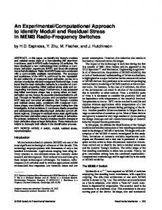
Figure 11: Evolution of the 3 left-most eigenvalues along the straight configuration eigenvalues grow more positive. However, the loss of stability here arises from the birth of complex eigenvalues. As the desired eigenvalues are also the smallest magnitude eigenvalues, we use the “shift-invert” strategy on the eigen problem (21) as shown below: · ¸ · ¸ ¸−1 · ¸ 4r0 · 4r0 K C M O  4θ 0  = µ−1  4θ 0  (45) CT O O O 4n0 4n0 Fig.11 depicts evolution of the three left-most eigenvalues as the load is varied. (Note that this is not a bifurcation diagram.) Observe that the 1st and 3rd eigenvalues approach each other as the load is increased until, at a critical load, they coalesce and then become complex (the latter not shown). As mentioned earlier, complex eigenvalues indicate that the straight solution becomes unstable. This is also known as Hamiltonian-Hopf bifurcation, e.g., [15]. The value of the critical load obtained here (19.9 in magnitude) compares well with the 2 1 critical load formula ( 2πLEI ≈ 19.74) given in ref. [2]. 2

6

A Note on Discretization Error and Convergence

Our algorithm requires an “accurate” represention of a static equilibrium. In general, this representation is in discrete form, coming from a numerical solver. It already inherits discretization error. We then form the global stiffness matrix K, mass matrix M and constraint matrix C. This requires the use of finite element interpolation functions and integration over each of the finite elements. 22

Thus, another error is introduced while forming these matrices. We first generate a family of solutions {uk } using the approach of Healey and −uk−1 k Mehta [12] until kukku < tol, indicating “convergence”. Here, subscript kk “k” corresponds to the order of refinement (number of elements used to generate equilibria) while k.k denotes L2 norm. For all the examples presented, the equilibrium solution converged within 150 elements. Once, we have a converged solution, we use linear shape functions and the mid-point integration rule for element integration during the Finite Element Assembly process to form the global matrices. Our algorithm further requires the columns of the constraint matrix C to be linearly independent. To check this, we first find the smallest singular value σmin of C. As entries in the C matrix are of the order of element size “h”, σmin is dependent on “h”. Therefore, we check the linear independence σmin of the columns of C by checking the ratio σmin signifies h . A small value for h that the columns of C are nearly dependent. Table 5 shows the ratio σmin for h different values of element size “h” in the second example 5.2 on “Stability of a Compressed Cable or DNA Strand”. Table 5: Element size(h) 0.12 0.06 0.04 0.03

7

σmin h

0.2105 0.2079 0.2219 0.2220

Concluding Remarks

A generalized computational approach to stability of static equilibria of nonlinearly elastic rods is presented. Based upon linearized dynamics, we are able to determine stability of static equilibria of a rod subjected to general boundary conditions, loadings and constraints - pointwise and/or integral type. We remark again that any approach based upon Jacobi’s conjugate-point method is necessarily limited to stability analysis of conservative problems with Dirichlet boundary conditions (or possibly Neumann boundary conditions [19]) and in the possible presence of integral constraints. Our proposed method also provides information about unstable eigen directions which may be utilized to stabilize a system via feedback control mechanism. We also present an efficient sparse-matrix-friendly algorithm to solve the associated eigenvalue problem. As mentioned at the end of Section 4, the algorithm has some limitations which can be overcome provided we have an efficient formula of the inverse of a “projected matrix” for the point-wise constrained case. However, ours has an advantage over other existing algorithms when applicable. Not only do we work efficiently with a reduced dimensional problem, but no purification strategy is required as all the spurious eigenvalues are eliminated. The computational cost associated with our algorithm is of the same order (O(n)) as that presented in ref. [20], while the approach presented herewith is applicable

23

to a much broader class of problems. We illustrated our method in the context of four examples. Of these, only the first, Example 5.1 “Perversion of a Telephone Cable” is directly amenable to the conjugate-point method. In the context of Example 5.2, we present a new “mixed” variational formulation for a general class of extensible, unshearable rods. This delivers a reduced representation for such rods, which is attractive for numerical computation of equilibria as well as for stability analysis. We intend to explore this formulation in more detail later. Indeed the formulation converts the pointwise unshearability constraints into integral type. Thus, with our new formulation in hand, it is also possible to analyze the second Example 5.2 “Stability of a Compressed Cable or DNA Strand” via the conjugate-point approach [20]. The same cannot be said for the other two Examples 5.3 and 5.4 - the former becuase of the boundary conditions and the latter due to the non-conservative loading. In the last Example 5.4, the “shift-invert” strategy with a real shift parameter could capture the eigenvalues with “sufficiently” small imaginary parts. Indeed, we only investigate the critical load at which real eigenvalues first “collide” and then become complex. But, in general, a complex shift may be required to capture eigenvalues with large imaginary parts [24]. Finally, the non-symmetric stiffness matrix, arising due to linearization of the boundary terms, is connected to its symmetric part via a low ranked matrix. This low rank connection could be beneficial in developing an algorithm which could exploit the niceties of symmetric problems and yet solve the non-symmetric problem.

Acknowledgments: We thank Charlie Van Loan for useful discussions concerning Section 4. This work was supported in part by the National Science Foundation through grant DMS-0707715.

References [1] S. S. Antman, Nonlinear Problems of Elasticity (Springer-Verlag, NY), 1995. [2] V. V. Bolotin, Nonconservative Problems of the Theory of Elastic Stability (Pergamon Press, Macmillan-NY), 1963 [3] L. Bozec, G. H. M. vander Heijden and M. Horton, Collagen Fibrils: Nanoscale Ropes, Biophysical Journal, Vol 92 (2007) 70-75 [4] K. A. Cliffe, T. J. Garratt and A. Spence, Eigenvalues of the discretized Navier-Stokes equation with application to the detection of Hopf bifurcations, Advances in Computational Mathematics 1(1993) 337-356 [5] D. Dichmann, Y. Li and J. H. Maddocks, Hamiltonian formulation and symmetries in Rod Mechanics, in Mathematical Approaches to Biomolecular Structure and Dynamics, ed. J. Mesirov, (Springer-Verlag, NY), 71-113

24

[6] E. J. Doedel, AUTO2000: Continuation and Bifurcation Software for Ordinary Differential Equations, 2000 [7] G. Domokos and I. Szeberenyi, A hybrid parallel approach to one-parameter nonlinear boundary value problems, Computer Assisted Mechanics and Engineering Sciences, Vol 11 (2001) 1-20 [8] G. Domokos and T. J. Healey, Multiple Helical Perversions of Finite, Intrinsically Curved Rods, International Journal of Bifurcation and Chaos, Vol 15, No. 3 (2005) 871-890 [9] G. H. Golub and C. F. Van Loan, Matrix Computations, The Johns Hopkins University Press, Baltimore, 3rd Edition [10] A. Goriely and M. Tabor, Nonlinear dynamics of filaments I. Dynamic instabilities, Physica D 10(1997) 20-44 [11] T. J. Healey, Material Symmetry and Chirality in Nonlinearly Elastic Rods, Math. Mech. Solids 7 (2002), 405-420 [12] T. J. Healey and P. G. Mehta, Straightforward Computation of Spatial Equilibria of Geometrically Exact Cosserat Rods, International Journal of Bifurcation and Chaos, Vol 15, No. 3 (2005) 949-965 [13] K. A. Hoffman, R. S. Manning and R.C. Paffenroth, Calculation of the stability index in parameter-dependent calculus of variations problems: Buckling of a twisted elastic strut, SIAM Journal on Applied Dynamical Systems, 1 (1). pp. 115-145 [14] R. B. Lehoucq and J. A. Scott, Implicitly Restarted Arnoldi Methods and Eigenvalues of the Discretized Navier Stokes Equations, Technical Report, 1997 [15] K. W. Macewen and T. J. Healey, A Simple Approach to the 1:1 Resonance Bifurcation in Follower-Load Problems, Nonlinear Dynamics 32: 143-159, 2003 [16] J. H. Maddocks, Stability of nonlinearly elastic rods, Archive for Rational Mechanics and Analysis, Vol 85 (1984), 311-354 [17] J. H. Maddocks, Stability and folds, Archive for Rational mechanics and Analysis, Vol 99 (1987), 301-328 [18] R. S. Manning, J. H. Maddocks and J. D. Kahn, A Continuum Rod Model of Sequence-Dependent DNA Structure, J. Chem Physics, [19] R. S. Manning, Conjugate Points Revisited and Neumann-Neumann Problems, Siam Review, Vol 51 (2009), 193-212 [20] R. S. Manning, K. A. Rogers and J.H. Maddocks, Isoperimetric conjugate points with application to the stability of DNA minicircles, Proc. R. Soc. Lond. A (1998) 454, 3047-3074 [21] J. F. Marco and E. D. Siggia, Bending and Twisting Elasticity of DNA, Macromolecules, 27 (1994), 981-988 25

[22] T. McMillen and A. Goriely, Tendril Perversion in Intrinsically Curved Rods, J. Nonlin. Sci., 12 (2002), 169-205 [23] K. Meerbergen and A. Spence, Implicitly Restarted Arnoldi With Purification For the Shift-Invert Transformation, Mathematics of Computation, Vol 66 (1997) 667-689 [24] K. Meerbergen, A. Spence and D. Roose, Shift-Invert and Cayley Transforms for Detection of Rightmost Eigenvalues of NonSymmetric Matrices, BIT Numerical Mathematics, 34(1994), 409-423 [25] D. R. Merkin, Introduction to the Theory of Stability (Springer), 1997 [26] J. Rommes, Arnoldi and Jacobi-Davidson methods for generalized eigenvalue problems Ax = Bx with singular B, Mathematics of Computation, Vol 77 (2008), 995-1015 [27] C. M. Papadopoulos, Nonlinear buckled states of Hemitropic Rods, Ph.D. Thesis, Cornell University, 1999 [28] J. C. Simo and L. Vu-Quoc, A Three-Dimensional Finite-Strain Rod Model. Part II: Computational Aspects, Comput. Methods App. Mech. Engrg 58 (1986) 79-116 [29] D. C. Sorensen, Implicit Application of Polynomial Filters in a K-Step Arnoldi Method, SIAM. J. Matrix Anal. & Appl. Volume 13, Issue 1(1992), 357-385 [30] R. S. Strichartz, The Way of Analysis (Jones and Bartlett), 1995 [31] D. Swigon, B. D. Coleman and I. Tobias, The Elastic Rod Model for DNA and itsApplication to the Tertiary Structure of DNA Minicircles in Mononucleosomes, Biophysical Journal, Vol 74 (1998), 2515-2530 [32] J. M. T. Thompson, G. H. M. vander Heijden and S. Neukirch, Supercoiling of DNA Plasmids: Mechanics of the generalized Ply, Proc. R. Soc. Lond. A (2002) 458, 959-985

26