available at BitBucket.org, where source code, downloadable jar (to easy install the plugin in Fiji), wiki and issue tracker are present. All the source code is ...
UNIVERSITY OF TRENTO Faculty of Mathematical, Physical and Natural Sciences
Degree in Biomolecular Sciences and Technologies Final Thesis
Development of a Computational Approach to Analyze Images of HIV Infected Cells
1st and 2nd Readers:
Graduant:
Francesca Demichelis Centre for Integrative Biology University of Trento
Gabriele Girelli
Daniele Arosio Biophysical Institute National Research Council
Academic Year 2011 – 2012
To deconvolve Or not to deconvolve? [anonymous microscopist]
TABLE OF CONTENTS 1
Introduction ................................................................................................................................................. 1
2
Methods ....................................................................................................................................................... 5 2.1
Sample preparation .............................................................................................................................. 5
2.2
Computational Methods ...................................................................................................................... 6
2.2.1
Images Storage ............................................................................................................................ 6
2.2.2
Deconvolution ............................................................................................................................. 6
2.3
3
Statistical Methods .............................................................................................................................. 7
2.3.1
Cohen’s kappa ............................................................................................................................. 7
2.3.2
Comparison with standard manual approach. .............................................................................. 9
Results ....................................................................................................................................................... 11 3.1
4
Developed Computational Approach ................................................................................................ 11
3.1.1
Input ........................................................................................................................................... 11
3.1.2
2D Elaboration for Particles Detection ...................................................................................... 11
3.1.3
3D Elaboration for Particles Detection ...................................................................................... 13
3.1.4
Filtering Steps ............................................................................................................................ 15
3.1.5
Output ........................................................................................................................................ 17
3.1.6
Nuclei Detection Workflow....................................................................................................... 18
3.1.7
PICs Detection Workflow ......................................................................................................... 20
3.1.8
Cytoplasm Detection ................................................................................................................. 22
3.2
Deconvolved and not-Deconvolved images analysis ........................................................................ 24
3.3
Statistical validation results ............................................................................................................... 24
Discussion.................................................................................................................................................. 29 4.1
Developed Approach Steps; .............................................................................................................. 29
4.1.1
Pre-Elaboration .......................................................................................................................... 29
4.1.2
2D Elaboration/Filtering ............................................................................................................ 29
4.1.3
3D Segmentation ....................................................................................................................... 30
4.2
To deconvolve or not to deconvolve?................................................................................................ 31
4.3
Cohen’s kappa ................................................................................................................................... 31
5
Conclusions ............................................................................................................................................... 33
6
Outlooks .................................................................................................................................................... 33
Acknowledgments ............................................................................................................................................. 35 References ......................................................................................................................................................... 37
i
ABBREVIATIONS INDEX AITA BF
Bright Field
CD
Centroid Distance
DA
Developed Approach
DI
Deconvolved Image
EDM
Euclidean Distance Map
GUI
Graphical User Interface
LAITA
ii
Automatic Intensity Threshold Algorithm
Local Automatic Intensity Threshold Algorithm
MA
Manual Approach
NDI
Not-Deconvolved Image
PIC
Pre-Integration Complex
POI
Particle Of Interest
PSF
Point Spread Function
ROI
Region Of Interest
SA
Standard Approach
SBR
Signal-to-Background Ratio
SNR
Signal-to-Noise Ratio
UEP
Ultimate Eroded Point
VOI
Volume Of Interest
IMAGES INDEX Image 3-1: an example of 4D stack xyzc with two channels: Blue (nuclei) and Green (PICs). ....................... 11 Image 3-2: panels (A) and (D) show a deconvolved nuclei image and a deconvolved PICs image respectively. (B) and (E) are obtained by images (A) and (D), in this order, after application of an automatic intensity threshold («Moments» method for nuclei, «Mean» method for PICs). Since nuclei were marked for the lamina, a step of filling was run, whose results are shown in panel (C). .......................................................... 12 Image 3-3: ROIs detected from the intensity thresholded image are here shown on the raw (deconvolved) image. ................................................................................................................................................................ 13 Image 3-4: CDs histogram automatically generated by PICsManager through RCaller. In this example the data are retrieved by a PICsManager run for nuclei detection. ......................................................................... 14 Image 3-5: CDs histogram automatically generated by PICsManager through RCaller. In this example the data are retrieved by a PICsManager run for intra-nuclear PICs detection. ..................................................... 14 Image 3-6: panel (A) and (B) shows two consecutive slices of an ideal z-stack, where particles borders and centroids are shown. (C) shows the two adjacent slices overlapped and in blue the minimum centroid distances, with which the ROIs are linked to build VOIs. ................................................................................ 15 Image 3-7: (A) shows a NDI blue channel, containing nuclei as POI. (B) shows the same image after nuclei detection with PICsManager. ROIs are shown in yellow before the outlier filter, after that the merged volumes should be discarded. .......................................................................................................................................... 16 Image 3-8: these graphs show the distribution of VOI areas over z-dimension. Specifically: graph (1) shows the VOIs prior to any filtering step, (2) shows VOIs after concavity filter, (3) shows the result of the outlier filter and (4) shows the VOIs after the discard of the two terminal ROIs. ........................................................ 17 Image 3-9: workflow colors legend. ................................................................................................................. 19 Image 3-10: nuclei detection workflow. Legend is Image 3-8. ........................................................................ 19 Image 3-11: PICs detection workflow. Legend is Image 3-8. .......................................................................... 20 Image 3-12: intra-nuclear PICs detection workflow, combines Image 3-10 andImage 3-11. .......................... 21 Image 3-13: the left panel shows the original bright field image, while the four panels on the right show the 2D-projection of intensity pixel variance calculated with four different measures. .......................................... 22 Image 3-14: from left to right the image shows (A) the original bright field image, (B) the 2D-projection of pixel intensity variance calculated as standard deviation, (C) cytoplasm ROI (yellow) obtained with Fiji’s ParticlesAnalyzer after Huang automatic intensity threshold was applied and (D) shows (yellow) the same ROI on the original bright field image after brightness/contrast automatic correction. ................................... 23 Image 3-15: two different stacks are shown, (A) has only green (PICs) and blue (nuclei) channel while (B) has also a bright field channel. Slices are z-ordered from left-to-right and top-to-bottom. .............................. 23 Image 3-16: nuclei (blue) and PICs (red) ROIs detected on not-deconvolved image (A) and deconvolved image(B). For the NDI analysis a Gaussian blur with «Moments» on whole stack for
was applied. Nuclei were detected with
while PICs were detected with «Mean» on whole stack for
. ............................................................................................................................................. 24
iii
TABLES INDEX Table 2-1: Cohen’s kappa arbitrary categorization proposed by Landis and Koch. ........................................... 8 Table 2-2: shows how the table for the Cohen’s kappa calculation has been compiled. P = particle; NP = notparticle. ................................................................................................................................................................ 9 Table 3-1: formulas of variance measures used in cytoplasm detection through bright field image projection of pixel intensity variance.
is the mean,
is the i-th quartile,
Table 3-2: Cohen’s kappa confidence intervals with a confidence of
. ....................................... 23 . Columns contains
respectively: (1) DA on not-deconvolved images (NDIs) versus MA on NDIs, (2) DA on deconvolved images (DIs) versus MA on NDIs, (3) DA on NDIs versus MA on DIs and (4) DA on DIs versus MA on DIs. Table is split between nuclei and PICs detection achieved through threshold calculated by whole-stack/single-slice method. Good values are highlighted in yellow, best value for each column is bolded. PICs data are obtained by PICsManager run for intra-nuclear PICs detection where nuclei were detected with «Moments» AITA. .. 25 Table 3-3: p-value of significance test of null hypothesis of no agreement for best Cohen’s kappa values. ... 26
iv
1 INTRODUCTION Classically virology studies have been performed in biological laboratories without any quantitative imaging instrument and with the main aim of understanding the biological mechanisms of a specific virus. Nowadays virologists often collaborate with biologists with imaging experience. The imaging approach to biology (bioimaging) allows to access 3D information, namely the spatial distribution of molecules like ions, proteins, or virions within single cells or specific sub cellular organelles. This study is focused on the development of a new computational approach to analyze the Human Immunodeficiency Virus (HIV) pre-integration complexes (PICs) in a three-dimensional (3D) fashion. A PIC is constituted by the provirus associated with viral proteins, e.g.: for HIV, the integrase IN protein is present in the PICs. Currently what’s know about PICs intracellular behavior is the following:
PIC has been estimated to be at least
PICs diffusion through the cytoplasm is very limited; upon entering the cell they tend to move
in diameter.
towards the nucleus using cytoskeleton (microtubules/actin) (McDonald, et al., 2002). Specifically microtubule-directed movement is saltatory, both retrograde and anterograde but with an overall directionality towards the nuclear compartment, while slower actin-directed transport is observed when reaching the perinuclear area (Arhel, et al., 2006).
Integrase seems to play an important role in nuclear import (Limòn, et al., 2002).
Once the perinuclear region is reached, PICs movements become quite restricted, probably due to the binding to the cytoplasmic region of nucleoporines (Arhel, et al., 2006).
Once entered the nucleus, PICs shows very slow and diffuse movements, which could be indicative of interactions with the chromatin (Arhel, et al., 2006). In fact, PICs selectively target decondensed chromatin in the nuclear periphery (Albanese, et al., 2008) suggesting a non-random distributed within the nuclei.
In summary very little is known about intra-nuclear PICs spatial distribution, and here we developed a new computational approach specifically for PICs detection would greatly help a study on this topic. In the current practice images are acquired, then analyzed by computer programs that often require intensive work by the user in order to get quantitative and/or qualitative information. These manual approaches, aside from being time-consuming, may lead to biased interpretation. New automatic or semi-automatic algorithms are needed to decrease the time required by the analysis and moreover to yield unbiased accurate analysis.
1
Many programs are currently available for image analysis that allow 3D rendering and basic 3D segmentation, tough they are mainly optimized for cell or nuclei detection, such as: BioImageXD, Icy, Vaa3D (Eliceiri, et al., 2012). Altogether these algorithms are not suited for the identification of sub-resolution viral particles, i.e.: PICs, detection through segmentation. The developed approach (DA) was implemented as a java plugin for Fiji, a distribution of the open-source software ImageJ (Schneider, et al., 2012) that is focused on biological-image analysis. What Fiji offers is an easy way to implement ImageJ plugins that can be shared with end user through an integrated update system (Schindelin, 2012). The DA was named PICsManager. In summary, here I will present a newly developed computational approach to identify HIV PICs and provide biologically relevant quantitative measurements, such as cytoplasm-nucleus ratio, spatial distribution and its validation upon current standard technique comparison.
2
2 METHODS 2.1 Sample preparation Intra-nuclear HIV-1 pre-integration complexes (PICs) can be visualized with the help of a trans-incorporation based pseudo-virus composed of a fluorescently marked protein fused with Vpr. The used pseudo-virus, namely VIN-GFP, is composed of the Vpr-Integrase-GFP fusion protein which is incorporated into maturing virions in producing cells through the interaction between Vpr and the p6 component of the viral Gag protein (Wu, et al., 1995). VIN-GFP pseudo-virus has been used to study the intra-nuclear properties of HIV-1 PICs (Albanese, et al., 2008) and appears to be an efficient tool for the evaluation of cellular factors involved in the nuclear import of viral complexes (Chris, et al., 2008). VIN-GFP viral supernatant equivalent to 0.2RT units were used to infect 100,000 Hela P4 cells plated on a glass coverslip through spinoculation at 1400g for 2 hours at 16°C. Spinoculated plates were transferred into the 37°C incubator for 2 hours for cell recovery, and later changed medium, at 6 hours post spinoculation, cells were briefly exposed to tripsin to remove membrane attached virions, and fixed with 2% PFA for 10 mins at 37°C which were further permeabilized with 0.1% Triton-x100 for 5 mins and blocked in a blocking buffer containing 0.1% tween-20 and 1% BSA for 20 mins. Cells were then incubated over night with blocking buffer containing a 1:100 dilution of Lamin A/C primary antibody (Santacruz), following subsequent washes with PBS 2x – 0.1% Triton x-100 1x - PBS 2x, cells were blocked with blocking buffer for 5 mins at room temperature prior to probing with secondary Donkey anti-Goat Alexa 633 antibody in the dark for 1 hour at room temperature. Secondary antibodies were washed PBS 2x – 0.1% Triton 1x – PBS 2x and incubated with blocking solution for an additional 5 mins. Coverslips were mounted on Vectashield (Vector Laboratories) mounting medium and observed under the 63x oil objective of the Leica SP-5 confocal microscope (Leica systems). Nuclear volumes were acquired with z-stack images that had a pixel resolution of alexa-633 (nuclear lamina) respectively with emissions ranges
for GFP and
in the x-y axis, exciting GFP (PICs) and and
wavelength laser line and collecting
for nuclear lamina.
5
2.2 Computational Methods 2.2.1
Images Storage
Acquired images were uploaded on the OMERO® (Open Microscopy Environment Remote Objects) database using the «OMERO.insight» client, which converts images into the standardized file format ‘.ome.tiff’. OMERO is hosted at the CNR-IBF facility, inside the FBK building in Povo (Trento, IT). This database allows to store and browse images and their associated metadata and to annotate them (through the «OMERO.web» interface); thus facilitating images (storage and) sharing (Swedlow, et al., 2009) processes. The images were then downloaded from the database and loaded onto Fiji through the «LOCI Bioformat Importer» plugin, converted into 8-bit type and analyzed. 2.2.2
Deconvolution
Deconvolution was performed with the Huygens Essential® software, and the result of each image deconvolution was uploaded onto the OMERO database. Huygens software allows both to compute a theoretical point spread function (PSF) based on known microscopic parameters and microscope model (e.g.: confocal, wide field) or to work out an experimental PSF from spherical bead images. While the latter is ideal, we opted for the first system because it’s less time-consuming. The degree of spreading of a single sub-resolution object (i.e.: PIC) is a measure for the quality of an optical system. The 3D blurry image of such a single point light source is usually called the Point Spread Function (PSF). The convolution substitute each sub-resolution object with its PSF while the de-convolution does the opposite, thus recovering a certain degree of the ground truth. Huygens Essential’s deconvolution is organized in the following steps: 1. Check microscope parameters to verify good sampling of the image: the estimated sampling is compared to the Nyquist ideal sampling. If images are under-sampled, i.e. below the ideal Nyquist rate, images are only slightly improved by deconvolution. (Scientific Volume Imaging B.V., s.d.). 2. Automatic inspect the image background. 3. Users input for the signal-to-noise ratio. 4. Apply proper deconvolution. The required signal-to-noise ratio (SNR) was calculated by using the following expression:
where
is the maximum value of intensity in a voxel and
is the intensity of a single photon hit. While
was automatically detected by the software as the maximum value in the image intensity histogram, has been calculated as the average intensity of five different single-pixel dots in the background with low intensity.
6
The use of bright field deconvolved images (BFDIs) to detect cytoplasm would have been interesting, but BF deconvolution non linearity of bright field imaging makes it tricky to apply (in linear imaging the image is the result of a linear convolution of the object distribution, namely the ground truth, and the point spread function, PSF). Also Huygens Professional® software allows to use the linear Tikhonov Miller algorithm to deconvolve bright field images. However, the algorithm application presented some inconveniences that we were not able to solve during the time of this work. As mentioned before, after downloading the images from OMERO, they were loaded onto Fiji (ImageJ 1.47c). In particular, the developed approach uses the following Fiji classes:
«ParticleAnalyzer» is used to identify particles in a binary (i.e.: thresholded) image. It allows to apply a filter on area (in virtual or physical units) or on circularity, then returns a RoiManager instance containing the generated ROIs and a ResultsTable instance containing measurements of the ROIs.
«AutoThresholder» is able to automatically calculate an intensity threshold value, using one of the many algorithms that Fiji provides.
«GenericDialog» is used to generate the tool GUI.
«RoiManager» is used to store the ROIs that the ParticleAnalyzer generates and allows ROI manipulation and measurement.
«ResultsTable» contains the ROI measurement obtained by the ParticleAnalyzer or the RoiManager.
As Fiji undergoes updates frequently, each class needs to be verified for proper use after software updates.
2.3 Statistical Methods 2.3.1
Cohen’s kappa
To measure the concordance between the DA and the standard approach (SA) we calculated the so-called Cohen’s kappa (
), which quantifies the normalized difference between the rate of agreement actually
observed and the rate of agreement that would be expected by chance. Cohen’s kappa assumes that two raters rate
where
entities into one of
mutually exclusive nominal categories as per the following formula:
is the overall frequency of agreement and
is the frequency of agreement expected by chance
(Banerjee, et al., 1999). Cohen’s kappa covers values between
and : it equals its maximum when the two
raters are fully concordant, a value of 0 indicates that the agreements are stochastic while it assumes its minimum value when the two raters never agree.
7
Cohen’s kappa interpretation tends to be arbitrary, so a categorization of Cohen’s kappa values (Landis & Koch, 1977) has been used to evaluate the results: Table 2-1: Cohen’s kappa arbitrary categorization proposed by Landis and Koch.
range of values Strength of Agreement Poor Slight Fair Moderate Substantial Almost Perfect In addition, for each
an approximate
confidence interval has been estimated (Kwiecien, et al., 2011) as
follows:
where the standard error is
We carried out also a significance test of null hypothesis of no agreement, i.e.: Under the null hypothesis
.
and the standard error become
means no agreement, so this is a one-side test. Since the confidence interval, kappa is poorly estimated when
8
or
is different between the test and the
but there is still evidence of agreement.
2.3.2
Comparison with standard manual approach
In order to validate the developed approach, we calculated the Cohen’s kappa between the new approach and the standard manual approach (MA) results. The MA was executed by a segmentation expert, from the Laboratory of Molecular Virology of CIBIO (Centre for Integrative Biology, Trento - IT), agnostic to the new algorithm. The standard approach consists of identifying each section of the particle of interest (POI) drawing a bounding rectangular region around it. We built the following table: Table 2-2: Cohen’s kappa calculation table for the comparison between automated and standard approach. P = particle; NP = not-particle.
#MA-P areas
#MA-NP areas
Total
#DA-P areas #DA-NP areas Total
First
was set equal to the number of ROIs detected by Fiji’s ParticleAnalyzer when run on the whole stack
with no circularity constraint. To get every detectable area present in the image, i.e.: POI’s sections along with areas that don’t belong to POIs, we detected areas equals or greater than 2px (i.e.: «#MA-P» areas (
).
) was generated by the segmentation expert and «#MA-NP» areas were calculated as . In parallel: «#DA-P areas» (
) was generated by the implementation of the
developed approach while «#DA-NP» areas were calculated as «DA-P areas» were manually compared to obtain the number
. Then «MA-P» areas and of common areas. The remaining
and
values were then calculated algebraically. After the table is compiled, we define categories,
where
where
and
,
is the number of
is the value in the cell at row and column , so that
is the observed probability of agreement while
is the probability of agreement expected if one of
the two raters was randomly rating. Finally
and its confidence interval can be calculated and the test can be executed.
9
3 RESULTS 3.1 Developed Computational Approach The developed computational approach is implemented as a plugin, PICsManager, for the image processing software Fiji. Its code is saved into a Mercurial repository which is available on BitBucket.org. PICsManager main functions are particle detection and analysis of their spatial distribution with quantitative measurements of volume and intensity. Here we describe the main components of the approach and of its use. 3.1.1
Input
PICsManager can analyze 3D/4D (i.e.: xycz or xyzc) 8-bit stack of images. If a 5D (time-lapse) stack of images is given as input the tool open a GUI in which the user can specify which frame has to be analyzed and extracting it, while the 8-bit limit is inherited by Fiji’s «ParticleAnalyzer» (used to identify objects in thresholded images). Both deconvolved and not-deconvolved images can be analyzed by PICsManager since at the beginning it allows to execute a Gaussian Blur step on the latter.
Image 3-1: an example of 4D stack xyzc with two channels: Blue (nuclei) and Green (PICs).
3.1.2
2D Elaboration for Particles Detection
The 2D elaboration for fluorescently stained particles detection is organized in three parts:
In the Pre-Elaboration step the format of the input image is evaluated: in the case of a 4D stack of images the first step is to extract the channel containing the Particles Of Interest (POIs), obtaining in this way a 3D (i.e.: xyz) stack of image with
slices. This step is obviously skipped if the input is a 3D stack of
images. Secondly, it is asked whether to apply a Gaussian Blur to the image: this is suggested only for not deconvoluted image (NDI) analysis since it makes POIs bigger by mixing signal, background and noise pixels. If this step is skipped on NDIs the detection will be prone to failure due to areas misdetection.
11
Segmentation’s aim is to detect the areas of the POIs (their sections) in each slice. To achieve this, Fiji’s «ParticleAnalyzer» class is used, requiring an 8-bit thresholded image. To do so, an automatic intensity threshold algorithm (Sezgin & Sankur, 2004) is run, returning a threshold which is then applied to the image. Fiji has seventeen different automatic threshold algorithms available amongst which the user can choose: Default, Huang, IJ_IsoData, Intermodes, IsoData, Li, MaxEntropy, Mean, MinError(I), Minimum, Moments, Otsu, Percentile, RenyiEntropy, Shanbhag, Triangle, Yen. The so-obtained binary image (containing only black and white pixels, i.e.: 0 and 255 of intensity) is passed to the ParticleAnalyzer which detects the POI sections (i.e.: Regions Of Interest, ROIs). Each ROI is characterized by centroid position (X, Y, Z), area, intensity measures and shape descriptors. After the detection, PICsManager allows the user to erode the ROIs by a certain percentage of the expected mean POI’s radius. (Ljosa & Carpenter, 2009)
Image 3-2: panels (A) and (D) show a deconvolved nuclei image and a deconvolved PICs image respectively. (B) and (E) are obtained by images (A) and (D), in this order, after application of an automatic intensity threshold («Moments» method for nuclei, «Mean» method for PICs). Since nuclei were marked for the lamina, a step of filling was run, whose results are shown in panel (C).
The Filtering step allows the user to apply filters on the ROIs based on their area and circularity. The area filter can be set both with pixel (i.e.: virtual units) and physical units (e.g.: circularity filter accepts an interval
12
where
,
) while the
is a perfect circle. The area filter is specifically
built upon the expected radius of the particle, which can be provided by input as an interval or as a fixed value
with its standard error
, in which case the interval becomes
This filter discards every ROI whose area
: it should be noted as, since
, the standard error of the area is
.
The detected ROIs are then passed on to the 3Ds elaboration part.
Image 3-3: ROIs detected from the intensity thresholded image are here shown on the raw (deconvolved) image.
3.1.3
3D Elaboration for Particles Detection
The 3D elaboration assigns each ROI to the corresponding POI and builds the POI’s volume: a ROI belongs at most to one POI, and a POI can have at most one ROI for each slice of the stack. To do so, the tool tries to link each ROI with a ROI in the following slice, in such a fashion to minimize their centroid distance (CD). PICsManager generates histograms (Image 3-4 and Image 3-5) of the calculated CDs and uses them to catch any error occurred during this step: specifically the near-zero peak height must be lower than its theoretical maximum
where
is the number of POIs (or number of build VOIs) and
the height of the near-zero peak in the case of
is the number of slices in the stack.
is
VOIs extending through the entire stack (i.e.: each VOI have
one ROI in every slice of the stack).
13
Image 3-4: CDs histogram automatically generated by PICsManager through RCaller. In this example the data are retrieved by a PICsManager run for nuclei detection.
Image 3-5: CDs histogram automatically generated by PICsManager through RCaller. In this example the data are retrieved by a PICsManager run for intra-nuclear PICs detection.
14
A threshold on the distances is automatically set to one fourth of the overall Feret’s diameter average, though a different value can be set by the user. The Feret’s diameter is defined as the longest distance between any two points along the ROI’s boundary, also known as maximum caliper. After this linking step the ROIs should be divided into small groups, namely POI volumes (VOIs). In other words, this step pieces together ROIs following the centroid of each volume through the slices of the z-stack. (Parthasarathy, 2012)
Image 3-6: panel (A) and (B) shows two consecutive slices of an ideal z-stack, where particles borders and centroids are shown. (C) shows the two adjacent slices overlapped and in blue the minimum centroid distances, with which the ROIs are linked to build VOIs.
For each VOI we can then define the variation area between two consecutive ROIs as where
,
is the number of ROIs in the VOI. The tool runs through each built VOI and split it
into two separate VOIs whenever 3.1.4
,
, where
is defined by input.
Filtering Steps
Besides the area and circularity filters of 2D elaboration, which are provided by the ParticleAnalyzer class itself, PICsManager allows the user to apply some filters on the VOIs (Image 3-8).
First of all VOIs are filtered based on their z-depth
which is equal to the number
selected VOI when calculated in virtual units (voxels,
) while is equal to
of ROIs in the (where
is the
distance between adjacent slices of the stack) when calculated in physical units. This filter discards those volumes whose z-depth
where
where
. We define the expected interval of z-depths as
is the average expected radius, while
, meaning that
, in other words
is built in such a way that
. 15
Also, another filter is available to discard every VOI with a non-concave distribution of a certain parameter dimension
(area, raw integrated density,…) through z-dimension. A parameter distribution on zis defined as concave when a certain value
of exists such that
In particular, it is possible to specify the size of the volume parts that should be in the monotonically increasing (or decreasing) branch. This filter can be useful when detecting particles whose volume is expected to be a sphere approximation.
Then, built volumes can be filtered for outlier presence of a certain parameter discarded if
is an outlier with
An «outlier» of a certain dataset
where
is the i-th quartile of
where
is defined as a value
and
Specifically, a VOI is
is the number of ROIs in the volume itself. such that
. This filter main purpose is to discard VOIs derived by
touching POIs that were detected as a single volume (Image 3-7).
Image 3-7: (A) shows a NDI blue channel, containing nuclei as POI. (B) shows the same image after nuclei detection with PICsManager. ROIs are shown in yellow before the outlier filter, after that the merged volumes should be discarded.
After the filtering steps, the two terminal ROIs of each VOI can be removed. This comes in handy, for example, when detecting nuclei for intra-nuclear PICs detection. In fact it’s assumed that at that point the nuclei are closed and every PICs detected in that section would be outside the nucleus.
16
Image 3-8: these graphs show the distribution of VOI areas over z-dimension. Specifically: graph (1) shows the VOIs prior to any filtering step, (2) shows VOIs after concavity filter, (3) shows the result of the outlier filter and (4) shows the VOIs after the discard of the two terminal ROIs.
3.1.5
Output
PICsManager outputs are:
a «log.dat» file containing information about every action executed by the tool;
a set of «plot.png» showing specific feature, specifically: o
centroid distances histogram shows the calculated centroid distances between ROIs in adjacent slices of the current stack;
o
area distribution on Z-dimension scatter-plot shows the area of each ROI over the slice index in which it’s contained, ROIs are divided into tracks based on which VOI they belong to;
o
raw integrated density distribution on Z-dimension scatter-plot shows the raw integrated density of each ROI over the slice index in which it’s contained, ROIs are divided into tracks based on which VOI they belong to; 17
a set of «data.csv» files, specifically: o
«resultsTables.csv» contains all the data about the detected ROIs: id, area, intensity mean, intensity standard deviation, intensity mode, intensity minimum, intensity maximum, centroid coordinates
, circularity, Feret’s diameter, calibrated
, center of mass coordinates
integrated density, intensity median, raw integrated density, stack position, Feret’s diameter end coordinates,
coordinate, Feret’s diameter angle, minimum Feret’s diameter, aspect ratio,
roundness, solidity, VOI’s id (this last only if available); o
«finalResults.csv» contains data about the detected VOIs: id, centroid coordinates
,
volume (both in virtual and physical units), intensity mean and raw integrated density; o
«count.csv» is generated only when detecting POIs inside other POIs, showing how many particles have been detected for each container particle;
o
«plot.csv» files containing the data required to draw the automatically generated «plot.png» files with other software of choice.
a «rois.zip» file containing the detected ROIs.
The «plot.png» files are automatically generated by PICsManager through R. RCaller package has been integrated in the tool to allow the communication between java and R language. This procedure has been chosen since it requires only a minimum number of other software to be present: R has to be installed on the machine where the plugin will run and the package ‘RUniversal’ has to be present. The R code used to automatically generate the «plot.png» files is stored into «log.dat». 3.1.6
Nuclei Detection Workflow
When detecting nuclei, ROIs are detected based only on the area (circularity is not considered). Specifically, we
used
an
,
detecting
ROIs
with
area
. Built VOIs were first discarded if , where
is the number of ROIs in the volume and
is the distance in physical units between two consecutive slices. VOIs were then split when
where
and
is the number of ROIs
in the volume. Each VOI is then passed through the filter for the concavity of the area distribution on Zdimension and, finally, checked for the presence of area outliers. If the input parameters are right, following this workflow (Image 3-10), the remaining VOIs are expected to correspond to the nuclei in the image.
18
Image 3-9: workflow colors legend.
Image 3-10: nuclei detection workflow. Legend is Image 3-9.
19
3.1.7
PICs Detection Workflow
For the PICs detection we used an
, detecting in this way ROIs with area
, no circularity filter has been applied. VOIs were then built and discarded if where
is the number of ROIs in the i-th volume (since
analyzed images, PICs were selected with a number of
in the
ROI in their volume).
Every VOI was then passed through two concavity filter of distribution on z-dimension: one for the ROI area and one for the raw integrated density. Only VOI that failed both filter were discarded, in other words there’s a logical or operation between the results of this two filters (Image 3-11).
Image 3-11: PICs detection workflow. Legend is Image 3-9.
20
When detecting intra-nuclear PICs the previously described operations are executed not on the whole image but on the nuclei VOIs, one per time. The final output is then combined together and the output files are generated (Image 3-12).
Image 3-12: intra-nuclear PICs detection workflow, combines Image 3-10 and Image 3-11.
21
3.1.8
Cytoplasm Detection
To detect the cytoplasm (i.e.: our POI) an alternative approach to cellular membrane staining has been tried, based on the use of a stack of bright field images of whole-cell. This method has been presented in (Selinummi, 2009) and consists in the following steps:
Given a 3D stack of images, a 2D projection is made where each pixel intensity corresponds to a measure of the intensity variation in the z-direction in the original stack in that specific
pixel location
(following image).
. Image 3-13: the left panel shows the original bright field image, while the four panels on the right show the 2Dprojection of intensity pixel variance calculated with four different measures.
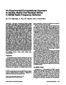
Four different variance measures have been tried for the projection: standard deviation, inter-quartile range, coefficient of variance and median absolute distance (Table 3-1)
An intensity threshold automatically calculated is then applied to the 2D projection and a ROI is then detected. This ROI is supposed to be a good approximation of the cytoplasm region (Image 3-14).
This approach seems to be good when cytoplasm is nearly constant through the stack. This was not our case (Image 3-15), so we started implementing the production of a stack of projections. In this approach a stack of slices is generated, from a bright field stack of
22
slices.
Table 3-1: formulas of variance measures used in cytoplasm detection through bright field image projection of pixel intensity variance. is the mean, is the i-th quartile, .
Measure
Formula
Standard Deviation
Interquartile Range Coefficient of Variance Median Absolute Distance
Image 3-14: from left to right the image shows (A) the original bright field image, (B) the 2D-projection of pixel intensity variance calculated as standard deviation, (C) cytoplasm ROI (yellow) obtained with Fiji’s ParticlesAnalyzer after Huang automatic intensity threshold was applied and (D) shows (yellow) the same ROI on the original bright field image after brightness/contrast automatic correction.
Image 3-15: two different stacks are shown; (A) has only green (PICs) and blue (nuclei) channel while (B) has also a bright field channel. Slices are z-ordered from left-to-right and top-to-bottom.
23
Each slice
in this newly generated stack is the intensity variance projection of the slices where
is a certain window-size selected by the user (
) and
with .
Currently this method has been partially implemented only for STD variance measure, so it would have been necessary to use fluorescent markers for cytoplasm detection but, since there was not enough time to prepare new biological sample, cytoplasm detection was not performed nor implemented into PICsManager.
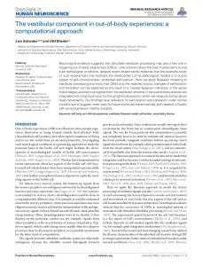
3.2 Deconvolved and not-Deconvolved images analysis Deconvolved and not-deconvolved images particle detection showed significantly different results after running the DA with the same parameters. In fact in the case of NDIs processing a Gaussian blur step is required to smooth the image. After Gaussian blur POIs appear to be bigger, so parameters should be consequently modified (i.e.:
should be increased) to adapt to this condition.
Image 3-16: nuclei (blue) and PICs (red) ROIs detected on not-deconvolved image (A) and deconvolved image (B). For the NDI analysis a Gaussian blur with was applied. Nuclei were detected with «Moments» on whole stack for while PICs were detected with «Mean» on whole stack for .
3.3 Statistical validation results The intra-nuclear PICs detection procedure has been applied to 4 z-stacks of images and their deconvolution results, each one with a nuclei-containing (blue) and a PICs-containing (green) channel. Here we present the statistical analysis of the results of the analysis only for one of the original z-stacks and its corresponding deconvolution result, on which the MA has been executed as well. Cohen’s kappa has been calculated for comparison between MA and DA applied on (not-) deconvolved images for both nuclei and PICs detection and with intensity threshold automatically calculated with whole-stack/single-slice method. The results of the statistical analysis are shown in Table 3-2. 24
Table 3-2: Cohen’s kappa confidence intervals with a confidence of . Columns contains respectively: (1) DA on not-deconvolved images (NDIs) versus MA on NDIs, (2) DA on deconvolved images (DIs) versus MA on NDIs, (3) DA on NDIs versus MA on DIs and (4) DA on DIs versus MA on DIs. Table is split between nuclei and PICs detection achieved through threshold calculated by whole-stack/single-slice method. Good values are highlighted in yellow, best value for each column is bolded. PICs data are obtained by PICsManager run for intra-nuclear PICs detection where nuclei were detected with «Moments» AITA.
Slice nuclei Method Default Huang IJ_IsoData Intermodes IsoData Li MaxEntropy Mean MinError Minimum Moments Otsu Percentile RenyiEntropy Shanbhag Triangle Yen Stack nuclei Method Default Huang IJ_IsoData Intermodes IsoData Li MaxEntropy Mean MinError Minimum Moments Otsu Percentile RenyiEntropy 25
Shanbhag Triangle Yen Slice PICs Method Default IJ_IsoData Mean MinError Percentile Stack PICs Method Huang Mean MinError Percentile For nuclei detection, the best automatic intensity threshold algorithms (AITAs) seems to be «Default» and «Moments», which retains a
in every case and appears to be the best method in 3 cases (over 8),
while for PICs detection the best one would seem to be «MinError» but since it usually fails to calculate the threshold value the best is «Mean» instead. For the greatest Cohen’s kappa in each table, a significance test of null hypothesis of no agreement (v.s.: 2.3.1) has been carried out and the p-values are shown in Table 2-1. Table 3-3: p-value of significance test of null hypothesis of no agreement for best Cohen’s kappa values.
26
POI
AITA
Option
Comparison
Nuclei
Default
Slice
DA-DI/MA-NDI
Nuclei
Otsu
Stack
DA-DI/MA-NDI
PICs
MinError
Slice
DA-DI/MA-DI
PICs
Mean/MinError
Stack
DA-DI/MA-DI
p-value
4 DISCUSSION 4.1 Developed Approach Steps; In summary, particle detection has been organized in the following steps: pre-elaboration, 2D elaboration/filtering and 3D elaboration/filtering. 4.1.1 Pre-Elaboration The intent of the pre-elaboration step is to convert the input image in a ‘standard format’, i.e.: in an 8-bit 3D (xyz) stack of images. Currently only the conversion from 4D/5D to 3D stack has been implemented, while the conversion to 8-bit image needs to be performed upfront by the user. In this part the user is also asked whether to apply or not apply a Gaussian blur, which is suggested only for NDIs. 4.1.2 2D Elaboration/Filtering The 2D segmentation is the most delicate step of this initial part as output differences have deep consequences on each of the following step. The DA first retrieves an intensity threshold value calculated by one of the AITA provided by Fiji. The threshold value is selected based on the intensity distribution of the image and ranges between the minimum and the maximum possible values (e.g.:
for 8-bit images).
Consequently they work differently when considering the whole stack intensity distribution or the intensity distribution of each slice singularly, creating a great number of possible algorithms to be used. In general, the whole stack method is highly recommended. The single slice method is recommended only when the environment conditions might have caused differences from a slice to another. The choice of the AITA is crucial. In fact the accuracy of the segmentation depends on the accuracy of the thresholding step as it drives the separation of the real signal from the background signal. Based on the selected algorithm, the user is asked to provide an ‘expected radius’ of the POIs, either as an interval or as a fixed value with standard error (v.s.: 3.1.2). Generally speaking, the better the quality of the images in terms of signal-to-background ratio (SBR), the easier the choice of the intensity threshold. Also, since the stain (or fluorescent marker) is never uniform, a local automatic intensity threshold algorithm (LAITA) would be preferred. The problem is that at the moment LAITAs are quite well developed only in the field of document analysis, «thus, there is a need to develop a thresholding method for the later, for accurate segmentation» (Phansalkar, et al., 2011). A new LAITA developed expressly for under-resolution (e.g.: PICs) particle detection would be of great benefit to this kind of study. The 2D filtering, which is based on area or circularity, is then subordinated to the choice of the most suitable AITA to identify a certain POI.
29
4.1.3 3D Segmentation Currently the step of volume reconstruction has been organized in such a way that branches in the VOI are split. That makes PICsManager unable to detect POIs that are not a sphere approximation. The presence of the near-zero peak in the CDs histograms (Image 3-4 and Image 3-5) allows us to build the volumes linking ROIs with nearest centroid. Also if the height of the near-zero peak exceeds its theoretical maximum (v.s.: 3.1.3) an error must have occurred during the volume building step. The first filter that is applied is based on the expected z-depth of the POI, which is deducted by the expected radius (v.s.: 3.1.4). Since it depends on the radius, this filter is strongly influenced by the chosen AITA. The filter based on the on-z-dimension distribution of a certain parameter is used:
In nuclei detection, since we are interested only in whole nuclei, to discard conical volumes (notconvex area distribution on z-dimension). In fact, partially recognized should have a not-concave area distribution, i.e.: a conical volume.
When detecting PICs to discard those with both conical volume and conical raw integrated density. We assume that, since pre-integration complexes are sub-resolution POIs, a VOI with concave area distribution on-z-dimension could appear as a conical volume. We try to compensate this effect passing the VOIs through a filter for the concavity of the raw integrated density distribution on-zdimension. Only the ROIs that safely pass through one of these two filters are maintained.
The last filter discards VOIs that contain at least one ROI with an outlier area (v.s.: 3.1.4) and, as abovementioned, its main purpose is to discard volumes derived by touching POIs. A possible alternative is the use of a watershed algorithm to separate the touching particles (Vincent & Soille, 1991). This «watershed» step consists of:
Calculation of the Euclidean Distances Map (EDM) which indicates, for each pixel in an object (can be calculated only on a binary image, i.e.: after the threshold), the shortest distance to the background (Danielsson, 1980).
Localization of ultimate eroded points (UEPs, peaks of the EDM).
Dilatation of UEPs until the background, or the edge of another dilating UEP, is reached.
This algorithm works best with smooth and convex objects that don’t overlaps. In our case it was not used since it was difficult to distinguish between VOI detected by merging POIs and the ‘normal’ ones and nuclei weren’t always convex (depending on the chosen AITA and on the use of DIs or NDIs). So, in the impossibility to apply the watershed algorithm, the outlier filter has been used instead. Noteworthy the step of volume splitting (based on
, v.s.: 3.1.3) is designed to avoid complete VOI
discard by this filter and comes in handy when POIs are touching near their tips.
30
4.2 To deconvolve or not to deconvolve? Besides the choice of an AITA, the use of DIs or NDIs influences the POIs size that PICsManager is able to detect. This is due to the fact that when analyzing NDIs the tool has to apply a Gaussian blur with a certain . The Gaussian blur determines the fusion of background, noise and signal causing the POIs to become bigger. It would be useful to implement into PICsManager the ability to modify the real expected POI’s radius, but at the moment the only workaround is for the user to input a wider
.
Also, if NDIs are used PICsManager is more prone to mistake noise or background for signal, while deconvolution result in higher SBR signals. If a circularity 2D filter is applied, DIs are best since one of the deconvolution results is a certain degree of recovery of the original particle’s form. On the other hand, deconvolution is a complex process that can result in worse images when wrong parameters are used. For example, images must be good sampled and SNR must be estimated well. If SNR is too high, there’s the risk that noise might just be enhanced. The signal-to-noise ratio must not be confused with the signal-to-background ratio (SBR). Signal and background may be defined as the averages in the high and low intensity regions while the noise discussed here is the «photon noise», i.e.: the intensity of a single photon hit. The best approach would be to analyze DIs acquired by a microscopist with deconvolution experience.
4.3 Cohen’s kappa Calculated Cohen’s kappa confidence intervals are shown in Table 3-2. The AITAs that are skipped in the table are those that returned a total number
of ROIs in the image equal to 0 when looking for POIs with
. From the values is clear that using AITAs with single-slice method the concordance of DA with MA is greater, whose results are shown in Table 3-3. Also Cohen’s kappa appears to be greater when comparing DA with MA executed on DIs. Clearly nuclei detection works better than PICs detection. The difficulty of PICs detection was expected, since are under-resolution POIs and the used images were not the most suitable for deconvolution (i.e.: some were under-sampled). It is advisable to execute this validation analysis again with better DIs and after implementation of automatic radius adjustment (v.s.: 4.2).
31
5 CONCLUSIONS In conclusion, a newly developed computational approach has been presented and validated. The validation results show a substantial agreement with the standard approach for the nuclei detection and a fair agreement for the PICs detection. Unfortunately there was not enough time to get to any biologically relevant measure, so this study possibly represent the first step of a long-term project to develop a computational approach capable of PICs exhaustive analysis. To get a feedback by the community and to share our results, the implemented method has been made available at BitBucket.org, where source code, downloadable jar (to easy install the plugin in Fiji), wiki and issue tracker are present. All the source code is published under the GNU General Public License of the Free Software Foundation (v.3 of the License or any later).
6 OUTLOOKS We envision that future work will include implementation of the following functions into PICsManager: Cytoplasm detection (expected to be very similar to nuclei detection). Stack-of-projection method for cytoplasm detection through bright field images. Measurement of nuclei-cytoplasm PICs ratio, highly relevant for the understanding of PICs nuclear import. Particle spatial distribution analysis. Specifically, PICs spatial distribution towards nuclear lamina for intra-nuclear distribution and ‘between-PICs’ for intra-nuclear PICs clustering. In addition, we expect to improve overall performance of PICsManager with respect to execution time and memory usage.
33
ACKNOWLEDGMENTS It is a pleasure to thank those who made this thesis possible. First of all many thanks go to Anna Cereseto, professor of Molecular Virology, she started my interest in the virology field and presented me to Francesca Demichelis and Daniele Arosio, who followed me through all the study. I owe them my deepest gratitude. I am indebted to many of my colleagues at CNR to support me, some are: Marta Marchioretto, Veronica De Sanctis, Francesco Rocca, Gaia Cecilia Santini, José Martinez Paredes, but my thanks go to all the CNR staff that helped me both with their professionalism and kindness. I thank my family, which supported me in so many ways. I would like to show my gratitude to Marica Anderle, who cried while eating a sandwich, and Benedetta Negri, whose support has been essential during this long summer (this study was carried out in summer). I am grateful to my roommate Elia ‘Pingu’ Bigliotti, who sustained me during the final year of my degree course, to my most precious friends: Matteo Ceresini, Francesco Ginelli, Alberto Coati and to the teacher that knows me best, Carla Vicenzoni. Lastly, I offer my regards and blessings to all of those who supported me in any respect during the completion of this project. ~Gabriele Girelli
35
REFERENCES Albanese, A., Arosio, D., Terreni, M. & Cereseto, A., 2008. HIV-1 Pre-Integration Complexes Selectively Target Decondensed Chromatin in the Nuclear Periphery. PLOS ONE, June, 3(6), p. e2413. Arhel, N. et al., 2006. Quantitative four-dimensional tracking of cytoplasmic and nuclear hIV-1 complexes. Nature Methods, October, 3(10), pp. 817-824. Banerjee, M., Capozzoli, M., McSweeney, L. & Sinha, D., 1999. Beyond kappa: A review of interrater agreement measures. The Canadian Journal of Statistics, 27(1), pp. 3-23. Chris, F. et al., 2008. Transportin-SR2 Imports HIV into the Nucleus. Current Biology, 26 August, Volume 18, pp. 1192-1202. Danielsson, P.-E., 1980. Euclidean distance mapping. Computer Graphics and Image Processing, November, 14(3), pp. 227-48. Eliceiri, K. W., Berthold, M. R. & Goldberg, I. G., 2012. Biological imaging software tools. Nature Methods, July, 9(7), pp. 697-710. Kwiecien, R., Kopp-Schneider, A. & Blettner, M., 2011. Concordance Analysis. Deutsches Ärzteblatt International, 108(30), pp. 515-21. Landis, R. T. & Koch, G. G., 1977. The Measurement of Observer Agreement for Categorical Data. Biometrics, March, 33(1), pp. 159-174. Limòn, A. et al., 2002. Nuclear Localization of Human Immunodeficiency Virus Type 1 Preintegration Complexes (PICs): V165A and R166A Are Pleiotropic Integrase Mutants Primarily Defective For Integration, Not PIC Nuclear Import. Journal of Virology, November, 76(21), pp. 10598-607. Ljosa, V. & Carpenter, A. E., 2009. Introduction to the Quantitative Analysis of Two-Dimensional Fluorescence Microscopy Images for Cell-Based Screening. PLOS Computational Biology, December, 5(12), p. e1000603. McDonald, D. et al., 2002. Visualization of the intracellular begaviour of HIV in living cells. Journal of Cell Biology, 11 November, 159(3), pp. 441-52. Parthasarathy, R., 2012. Rapid, accurate particle tracking by calculation of radial symmetry centers. Nature Methods, July, 9(7), pp. 724-26. Phansalkar, N., More, S., Sabale, A. & Joshi, M., 2011. Adaptive Local Thresholding for Detection of Nuclei in Diversity Stained Cytology Images. Kerala, s.n., pp. 218-220. Schindelin, J., 2012. Fiji: an open-source platform for biological-image analysis. Nature Methods, July, 9(7), pp. 676-82. Schneider, C. A., Rasband, W. S. & Eliceiri, K. W., 2012. NIH Image to ImageJ: 25 years of image analysis. Nature Methods, 9(7), pp. 671-75.
37
Scientific Volume Imaging B.V., n.d. Sampling and sampling density. [Online] Available at: http://www.svi.nl/SamplingDensity [Accessed 19 September 2012]. Selinummi, J., 2009. Bright Field Microscopy as an Alternative to Whole Cell Fluorescence in Automated Analysis of Macrophage Images. PLOSone, October, 4(10), p. e7497. Sezgin, M. & Sankur, B., 2004. Survey over image thresholding techniques and quantitative performance evaluation. Journal of Electronic Imaging, January, 13(1), pp. 146-165. Swedlow, J. R., Goldberg, I. G. & Eliceiri, K. W., 2009. Bioimage Informatics for Experimental Biology. Annual Reviews of Biophysics, Volume 38, pp. 327-46. Vincent, L. & Soille, P., 1991. Watershed in Digital Spaces: An Efficient Algrithm Based on Immersion Simulations. IEEE Transactions on Pattern Analysis and Machine Intelligence, June, 13(6), pp. 583-98. Wu, X. et al., 1995. Targeting Foreign Proteins to Human Immunodeficiency Virus Particles via Fusion with Vpr and Vpx. Journal of Virology, June, 69(6), pp. 3389-98.
38