A Graph Cut Algorithm for Generalized Image Deconvolution. Ashish Raj. UC San ..... parison of min-cut/max-flow algorithms for energy mini- mization in vision.
A Graph Cut Algorithm for Generalized Image Deconvolution Ramin Zabih Cornell University Ithaca, NY 14853
Ashish Raj UC San Francisco San Francisco, CA 94143
Abstract
simply note that it is a linear inverse problem with sparse non-negative H. Inverse problems of this form are ill-posed, and are typically solved by minimizing a regularized energy function [11]. The energy of a solution x is given by
The goal of deconvolution is to recover an image x from its convolution with a known blurring function. This is equivalent to inverting the linear system y = Hx. In this paper we consider the generalized problem where the system matrix H is an arbitrary non-negative matrix. Linear inverse problems can be solved by adding a regularization term to impose spatial smoothness. To avoid oversmoothing, the regularization term must preserve discontinuities; this results in a particularly challenging energy minimization problem. Where H is diagonal, as occurs in image denoising, the energy function can be solved by techniques such as graph cuts, which have proven to be very effective for problems in early vision. When H is non-diagonal, however, the data cost for a pixel to have a intensity depends on the hypothesized intensities of nearby pixels, so existing graph cut methods cannot be applied. This paper shows how to use graph cuts to obtain a discontinuitypreserving solution to a linear inverse system with an arbitrary non-negative system matrix. We use a dynamically chosen approximation to the energy which can be minimized by graph cuts; minimizing this approximation also decreases the original energy. Experimental results are shown for MRI reconstruction from fourier data.
||y − Hx||22 + G(x),
which is the sum of a data term and a smoothness term. The data term forces x to be compatible with the observed data, and the smoothness term G(x) penalizes solutions that lack smoothness. This approach can be justified on statistical grounds, since minimizing equation (2) is equivalent to maximum a posteriori estimation [11] assuming Gaussian noise. The energy is proportional to the negative logarithm of the posterior: the data term comes from the likelihood, and the smoothness term comes from the prior. A wide variety of algorithms have been developed to minimize equation (2) when G imposes global smoothness [12]. However, global smoothness is inappropriate for most vision problems, since most underlying quantities change slowly across most of the image, but have discontinuities at object boundaries. As a result, some form of discontinuitypreserving G is required, which makes the energy minimization problem NP-hard [4]. A natural class of discontinuity-preserving terms is
1. Generalized Image Deconvolution
GM RF (x) =
�
V (xp , xq ).
(3)
(p,q)∈N
The goal of image deconvolution is to recover an image x from its convolution with a known blurring function h. This is equivalent to solving the linear inverse problem [1] y = Hx
(2)
The neighborhood system N consists of pairs of adjacent pixels, usually the 4-connected neighbors. The smoothness cost V (l, l� ) gives the cost to assign l and l � to neighboring pixels. Typically the smoothness cost has a discontinuitypreserving form such as V (l, l� ) = min(|l−l� |, K) for some metric |·| and constant K. Such a smoothness term incorporates discontinuity-preserving priors, which can be justified in terms of Markov Random Fields [8]. We will assume throughout that V has a discontinuity-preserving form, as otherwise GM RF would be merely another way of imposing global smoothness.
(1)
for x given y, where H is the convolution matrix corresponding to h. In this paper we consider the generalized image deconvolution problem, where H is an arbitrary nonnegative matrix. This generalization is motivated by an important problem in medical imaging, namely the reconstruction of MRI images from fourier data. We will discuss this problem in more detail in section 5.1; for the moment, we 1
1.1. Energy function definition
Convex optimization techniques can be generalized to handle certain MRF-based smoothness terms under restricted assumptions. [5] presents a compound Gaussian MRF model for image restoration. They introduce additional parameters describing edge discontinuities into the MRF prior model, but the underlying image is assumed to have a Gaussian distribution enabling the use of Tikhonovregularized inversion. [2] considers generalized Gaussian MRF models, which handle the (highly restricted) class of non-convex priors which can be turned into Gaussian priors by a non-linear transformation of image intensities. These approaches, while interesting, cannot be generalized to discontinuity-preserving smoothness terms like G M RF . It is also possible that an energy function like ours could be minimized by a fast algorithm that is not based on graph cuts, such as loopy belief propagation (LBP) [10]. LBP is a method for inference on graphical models, which has been reported to produce results that are comparable to graph cuts [16]. It is not clear whether or not LBP could be used for the energy function we examine, as it is in a different form than the ones where LBP has been applied (such as [16]). In addition, LBP is not guaranteed to converge on problems that arise in early vision, due to the highly loopy structure of the neighborhood system. In contrast, graph cut energy minimization algorithms have well-understood convergence properties, and (as we will demonstrate) can be modified to minimize our energy function. A related problem is addressed in [17] using LBP. They are concerned with reducing the number of potential labels that a pixel can have, in order to make graphical inference more efficient. While they do not minimize a new class of energy functions, their technique can be used to perform deconvolution. Their method relies on learning, and uses LBP for inference, while we do not use learning and use graph cuts for energy minimization. While their use of learning is innovative, there is an advantage to our non-learning based approach, since for many applications it may be difficult to obtain a representative training set.
The problem we address is to efficiently minimize E(x) = ||y − Hx||22 + GM RF (x).
(4)
When H is diagonal, as in image denoising, the data term has a restricted form that makes it computationally tractable to minimize E. Specifically, � ||y − Hx||22 = (yp − Hp,p xp )2 , (5) p
which means that the data cost for the pixel p to have the hypothesized label (i.e., intensity) x p only depends on x p and yp . With such an H, the energy E can be efficiently minimized by graph cuts, which have proven to be very effective for pixel labeling problems such as stereo [15]. Graph cuts, however, can only be applied to certain energy functions [7]. We will demonstrate in section 3 that existing graph cut energy minimization methods cannot be applied when H is non-diagonal. Intuitively, this is because the data cost for a pixel to have a label depends on the hypothesized labels of other nearby pixels. Many important problems involve a non-diagonal system matrix whose elements are zero or positive. Examples include motion deblurring and the reconstruction of MRI images from raw Fourier data.
1.2. Overview In this paper, we propose a new graph cuts energy minimization algorithm which can be used to minimize E when H is an arbitrary non-negative matrix. We begin with a brief survey of related work. In section 3 we give some technical details of graph cuts, and show that existing methods cannot minimize E when H is non-diagonal. In section 4 we show that a dynamically chosen approximation to E can be minimized with graph cuts, and that minimizing the approximation also decreases E. Section 5 demonstrates experimental results for MRI reconstruction.
3. Graph Cuts for Non-diagonal H
2. Related Work
In the last few years, efficient energy minimization algorithms using graph cuts have been developed to solve pixel labeling problems [4]. These algorithms have proven to be very effective; for example, the majority of the top-ranked stereo algorithms on the Middlebury benchmarks use graph cuts for energy minimization [15]. The most powerful graph cut method is based upon expansion moves.1 Given a labeling x and a label α, an α-expansion χ = { χp | p ∈ P } is a new labeling where χp is either xp or α. Intuitively, χ
There are many optimization techniques to solve equation (2) when G imposes global smoothness; examples include Preconditioned Conjugate Gradient (PCG), Krylovspace methods, and Gauss-Siedel [12]. Unfortunately, these convex optimization methods cannot be applied when the smoothness term is of the discontinuity-preserving form given by G M RF . This is not surprising, since the most of these methods use some variant of local descent, while pixel labeling problems with discontinuity-preserving smoothness terms are NP-hard [4].
1 The other graph cut methods either have a running time that is quadratic in the number of intensities [4, Sec. 4] or are cannot handle discontinuity-preserving smoothness terms [6].
2
is contructed from x by giving some set of pixels the label α. The expansion move algorithm picks a label α, finds the lowest cost χ and moves there. The algorithm converges to a labeling where there is no α-expansion that reduces the energy for any α. The key step in the expansion move algorithm is to compute the α-expansion χ that minimizes the energy E. This can be viewed as a binary energy minimization problem, since during an α-expansion each pixel either keeps its old label or moves to the new label α. An α-expansion χ is equivalent to a binary labeling b = { b p | p ∈ P } where � xp iff bp = 0, χp = (6) α iff bp = 1.
(Recall that the equivalence between χ and b is given by equation (6)). It is shown in [7] that if V is a metric B2 satisifies equation (8). As a result B is regular, and so the expansion move algorithm can be applied. Fortunately, many discontinuity-preserving choices of V are metrics (see [4] for details). However, the situation is very different when H is nondiagonal. Consider �N the correlation matrix of H defined by RH (p, q) = r=1 Hr,p Hr,q . We can then write � �� ||y − Hx||22 = yp2 − 2 ( yq Hq,p)xp +
Just as for a labeling χ there is an energy E, for a binary labeling b there is an energy B. More precisely, assuming χ is equivalent to b, we define B by
The first three terms in (11) depend only on a single pixel while the last term depends on two pixels at once. As a result, when H is non-diagonal the second term in (7) is � � 2RH (p, q)χp χq + V (χp , χq ). (12)
� p
B(b) = E(χ).
(p,q)
We have dropped the arguments x, α for clarity, but obviously the equivalence between the α-expansion χ and the binary labeling b depends on the initial labeling x and on α. Since we will focus on problems like image restoration or denoising, we will assume in this paper labels are always intensities, and use the terms interchangeably. In summary, the problem of computing the α-expansion that minimizes E is equivalent to finding the b that minimizes B. The exact form of B will depend on E. Graph cuts can be used to find the global minimum of B, and hence the lowest cost α-expansion χ, as long as B is of the form � � B(b) = B1 (bp ) + B2 (bp , bq ). (7) p
+
q
�
RH (p, q)xp xq .
(11)
(p,q)
(p,q)∈N
P ROOF : The regularity condition is that for any α and pixel pair (p, q) RH (p, q)(α2 + xp xq − αxp − αxq ) ≤ 0.
(13)
RH is non-negative by construction, and the polynomial in α factors into (α − x p )(α − xq ). So equation (13) holds iff xp ≤ α ≤ xq .
(14)
This is clearly invalid for arbitrary x p, xq and α.
Here, B1 and B2 are functions of binary variables; the difference is that B1 depends on a single pixel, while B 2 depends on pairs of pixels. It is shown in [7] that such a B can be minimized exactly by graph cuts as long as
Thus, the optimal α-expansion can only be computed on those pixels { p | ∀q x p ≤ α ≤ xq }. This is a small subset of the image.
4. Approximating the Energy
(8)
If B2 satisfies this condition, then B is called regular (there is no restriction on the form of B 1 ). When H is diagonal the data term is given in (5), which only involves a single pixel at a time, while the smoothness term involves pairs of pixels. Hence B1 comes from the data term, while B2 comes from the smoothness term: � (yp − Hp,p xp )2 if bp = 0, (9) B1 (bp ) = (yp − Hp,p α)2 if bp = 1,
We now demonstrate how to use the graph cuts to minimize our energy function for arbitrary non-negative H. Our approach is to minimize a carefully chosen approximation to the original energy E. The approximation is chosen dynamically (i.e., it depends upon x and α), and the α-expansion that most decreases the approximation can be rapidly computed using graph cuts. While we cannot guarantee that we find the best α-expansion for the original energy function E, we can show that decreasing our approximation also decreases E. As before, we will use the expansion move algorithm with a binary energy function B. We will assume that V is
while B2 (bp , bq ) = V (χp , χq ).
p
Theorem 1 When H is non-diagonal, the binary cost function B(b) is not regular.
p,q
B2 (0, 0) + B2 (1, 1) ≤ B2 (1, 0) + B2 (0, 1).
p
R2H (p, p)x2p
(10) 3
energy when we move from x to χ under the two different energy functions can be written as
a discontinuity-preserving metric, which means that we can write B(b) = Bregular (b) + Bcross (b), where Bcross (b) =
�
2RH (p, q)χp χq
ΔB = B(b) − B(0),
(15)
(p,q)
¯ (p,q)∈R
The function Δ(χp, χq ) is defined by ⎧ 0 ⎪ ⎪ ⎪ ⎨ xq (xp − α) Δ(χp , χq ) = ⎪ x p (xq − α) ⎪ ⎪ ⎩ x +x 2α( p 2 q − α)
= x p , χq = x q , = α, χq = xq , = xp , χq = α, = χq = α. (19) In order to reduce the value of the original energy function, we need ΔB ≤ 0. It suffices to show that the second term in equation (18) is positive. Let us define the set of pixel pairs
¯ | xp < α, xq < α , R� = (p, q) ∈ R
R = { (p, q) | xp ≤ α ≤ xq }. Let Nd be the set of all pixel pairs interacting together via the cross data cost (15). For convenience, we wil also define ¯ = Nd \ R, which is the intersection of N d and the comR plement of R. We can split the pairs of pixels (p, q) into ¯ We will use an approximation those in R and those in R. ¯ for those pixels in R.
+
�
C = { p | ∃q s.t. (p, q) ∈ R� }.
(20)
C is important because if we do not modify pixels in C, then reducing our modified energy reduces the original energy. Theorem 3 Let x be an initial labeling and consider the α-expansion χ corresponding to the binary labeling b. Suppose that b does not modify the label of any pixel in C, i.e. ∀p ∈ C, bp = 0. Then if b decreases our modified energy ˆ < 0), it also decreases the original energy (i.e., (i.e., ΔB E(χ) < E(x).
2RH (p, q)χp χq
(p, q) ∈ R RH (p, q)(xpχq + χp xq )
χp χp χp χp
and the set of pixels
We begin by approximating B cross by �
(17)
ˆ so We can use graph cuts to find the b that minimizes B, ˆ ΔB < 0. We wish to show that this results in a decrease in the original energy function, i.e. ΔB < 0. ˆ we can write Using the definitions of B, B � ˆ = ΔB + ΔB RH (p, q)Δ(χp, χq ). (18)
are the only terms that are not known to be regular. Graph cuts cannot be used because there will be pairs (p, q) that do not satisfy equation (14), and as a result B is not regular. In the following analysis we will omit the potential terms that come from V (xp , xq ), since our aim is to obtain an approximation which is valid regardless of the choice of V . In general, if these terms are large they can potentially cause some otherwise irregular pairs to become regular. However, our approximation should not rely on this occurring since the choice of V reflects prior information about the importance and form of image smoothness, and should be as unconstrained as possible. We will create a regular approximation B � and minimize it instead of B. The construction proceeds in two steps; ˆ and then we first, we introduce an initial modification B, � ˆ use B to build B . Let R denote the set of pairs (p, q) that obey equation (14) at the current labeling x, i.e.
ˆcross (b) = B
ˆ = B(b) ˆ − B(0). ˆ ΔB
(16)
¯ (p, q) ∈ R
P ROOF : If p �∈ C, then for some neighbor q at least one of xp , xq is greater than α. If both x p > α and xq > α, then Δ(χp , χq ) ≥ 0, since all of the cases in equation (19) are non-negative. If α lies between x p , xq then (p, q) ∈ R.
ˆ Our initial approximation is B(b) = Bregular (b) + ˆ Bcross (b). It is straightfoward to show that we can use graph cuts with this approximation (the proof appears in [14]).
ˆ since minWe will need a better approximation than B, ˆ is sound, but not practical. In practice, C will imizing B be too large for fast convergence, since pixels in C do not change. We will further modify the energy to allow all pixels to potentially change, hence increasing the convergence speed. Our final approximation is � ˆ + B � (b) = B(b) λbp , (21)
ˆ Theorem 2 The energy function B(b) is regular. The obvious question is whether decreasing our modiˆ results in a decrease in the original fied energy function B energy function B. Consider an initial labeling x and an α-expansion χ. Both χ and the input labeling x correspond to binary labelings; χ corresponds to b, and x corresponds to the zero vector, which we will write as 0. The change in
p∈C
4
where λ is a constant. This imposes a cost of λ for a pixel in C to increase in brightness to α. Notice that the new cost only depends on a single pixel at a time, so B� is regular and we can use graph cuts to rapidly compute its global minimum. The following theorem, whose proof is supplied in [14], shows that reducing B � reduces B. Theorem 4 Let x be an initial labeling and consider the αexpansion χ corresponding to the binary labeling b. Then if b decreases our modified energy B� , it also decreases the original energy (i.e., E(χ) < E(x)).
Figure 1. Left: sensitivity map for a coil at the top left of the object. Right: system matrix for parallel imaging, shown for L = 4 coils. Nonzero entries, which come from the sensitivity maps, are shown as circles.
Our algorithm, then, replaces B by the approximation B � and uses graph cuts to find the global minimum of B � . We are guaranteed that this decreases the original energy E which we wish to minimize.
commonly in this application, where the system matrix H encodes the fourier transform. A particularly compelling application lies in a fast scanning technique called parallel imaging, which has previous been solved without imposing spatial smoothness. Fast scanning is extremely important in MR, because MR is known to be very sensitive to motion artifacts [9]. Parallel imaging techniques, such as SENSE [13] and its variants, significantly accelerate acquisition speed by subsampling in fourier space. To overcome the aliasing that subsampling induces, multiple receiver coils are used. The image created by a coil is brightest at pixels near the coil and falls away smoothly with distance from the coil. By scanning a uniform phantom, it is possible to compute the multiplicative factor that each coil applies to each intensity (this is called a sensitivity map, and an example is shown at left in figure 1). Given the sensitivity maps and the aliased coil outputs, the well-known SENSE algorithm [13] reconstructs the un-aliased image using least squares. Least squares, of course, computes the maximum likelihood estimate, which corresponds to having no smoothness term whatsoever. The problem of reconstructing the un-aliased image is an example of the generalized deconvolution problem, with the observation y computed from the coil outputs and the system matrix H computed from the sensitivity maps. Assume there are L coils and that each coil subsamples by a factor of R (which reduces scan time by a factor of R). Standard acquisition protocols perform regular cartesian sampling in fourier space. Taking the inverse fourier transform results in a linear inverse problem with a sparse system matrix of the form shown at right in figure 1 (see [13] for details). In parallel imaging the non-zero elements of the system matrix are sensitivity map entries, which are non-negative. (A precise definition of the system matrix for parallel imaging is given in [14].)
5. Experimental results Our approach is valid for any non-negative H, which covers the vast majority of linear inverse problems in vision.2 Our experimental results focus the important problem of reconstructing MRI images from fourier data. Running time for our method was approximately 2 minutes on 256 by 256 images for a Matlab implementation ([3] provides evidence that the speed of graph cut methods scales linearly with the number of pixels). Since there are very few methods that can minimize our energy function, we compared against an energy function with the first derivative as the smoothness term G in equation (2). Such an energy function is expected to produce oversmoothing, but has the advantage that it can be minimized by standard numerical methods such as PCG. As a result, it is representative of a large class of approaches to linear inverse problems. Note that PCG is subject to various numerical issues such as round-off error, which our method avoids (since we do not perform any floating point calculations). Parameters for our method and for PCG were experimentally chosen from a small number of trial runs. In the following experiments we used the truncated linear model for potential functions between neighbours. Further details of the exact choices of parameters are given in [14], along with experimental evidence that our method can also perform motion deblurring.
5.1. The MRI reconstruction problem Reconstructing MRI’s from the raw fourier data generate by an MR scanner is an important problem in medical imaging [9]. Generalized deconvolution problems arise 2 Our method actually covers a larger group of system matrices; we only require that R H is non-negative.
5
5.2. MRI reconstruction results
edges in the graph would increase, which asymptotically should produce a linear increase in running time. Yet for several 3D vision problems [3] found that going from a 6-connected neighborhood system to a 26-connected one roughly doubled the running time. It is thus unclear how significant an issue the running time would be.
In figure 2 we present the reconstructed images obtained by our graph cut method, as well as standard SENSE. In order to perform a comparison with a “gold standard”, we obtained these results from a normal-speed scan. Ideally, the parallel imaging methods should be able to reconstruct the same image from heavily sub-sampled inputs, which can be obtained much faster. In our experiments the sub-sampling factor, R, was chosen to be 3, with L = 4 coil outputs. Results are shown for both a phantom and a patient’s knees. One would expect to see better spatial smoothing with our method than with SENSE, and this is quite obvious in the phantom images in the top row. The patient data also appears to be somewhat improved by our method, although the differences are more subtle. In the zoomed in region of the patient’s knee shown in the bottom row, the edge definition produced by our method seems somewhat better than SENSE, although it is definitely not as good as the original (non-accelerated) version. In terms of PSNR, our method gives an improvement on the phantom image (SENSE PSNR: 24.3; our PSNR: 26.1), while on the patient image our PSNR numbers are slightly worse (SENSE PSNR: 29.3; our PSNR: 29.2).
References [1] M. Beretro and P. Boccacci. Introduction to Inverse Problems in Imaging. Institute of Physics, 1998. [2] C. Bouman and K. Sauer. A generalized Gaussian image model for edge preserving MAP estimation. IEEE Transactions on Image Processing, 2(3):296–310, 1993. [3] Y. Boykov and V. Kolmogorov. An experimental comparison of min-cut/max-flow algorithms for energy minimization in vision. IEEE Trans Pattern Anal Mach Intell, 26(9):1124–1137, 2004. [4] Y. Boykov, O. Veksler, and R. Zabih. Fast approximate energy minimization via graph cuts. IEEE Transactions on Pattern Analysis and Machine Intelligence, 23(11):1222– 1239, 2001. [5] M. A. Figueiredo and J. M. Leitao. Unsupervised image restoration and edge location using compound GaussMarkov random fields and the MDL principle. IEEE Transactions on Image Processing, 6(8):1089–1102, 1997. [6] H. Ishikawa. Exact optimization for Markov Random Fields with convex priors. IEEE Transactions on Pattern Analysis and Machine Intelligence, 25(10):1333–1336, 2003. [7] V. Kolmogorov and R. Zabih. What energy functions can be minimized via graph cuts? IEEE Trans Pattern Anal Mach Intell, 26(2):147–59, 2004. [8] S. Li. Markov Random Field Modeling in Computer Vision. Springer-Verlag, 1995. [9] Z.-P. Liang and P. C. Lauterbur. Principles of Magnetic Resonance Imaging: A Signal Processing Perspective. IEEE press, 1999. [10] J. Pearl. Probabilistic reasoning in intelligent systems: networks of plausible inference. Morgan Kaufmann, 1988. [11] T. Poggio, V. Torre, and C. Koch. Computational vision and regularization theory. Nature, 317:314–319, 1985. [12] W. Press, S. Teukolsky, W. Vetterling, and B. Flannery. Numerical Recipes in C. Cambridge, 1992. [13] K. P. Pruessmann, M. Weiger, M. B. Scheidegger, and B. Peter. SENSE: sensitivity encoding for fast MRI. Magnetic Resonance in Medicine, 42(5):952–962, 2001. [14] A. Raj. Improvements in Magnetic Resonance Imaging using Information Redundancy. PhD thesis, Cornell, 2005. [15] D. Scharstein and R. Szeliski. A taxonomy and evaluation of dense two-frame stereo correspondence algorithms. International Journal of Computer Vision, 47:7–42, 2002. [16] M. F. Tappen and W. T. Freeman. Comparison of graph cuts with belief propagation for stereo, using identical MRF parameters. In International Conference on Computer Vision, pages 900–907. 2003. [17] M. F. Tappen, B. C. Russell, and W. T. Freeman. Efficient graphical models for processing images. In IEEE Conference on Computer Vision and Pattern Recognition, pages II: 673–680. 2004.
6. Conclusions We have shown that graph cut algorithms can efficiently compute a discontinuity-preserving solution to linear inverse problems with a non-negative system matrix H. The obvious extension of our work would be to generalize our results to arbitrary H. We would only need to handle the case where RH can be negative; it seems plausible that this could be done by further refining our approximation to the original energy function. Linear inversion problems where RH can be negative, however, do not appear to arise often in computer vision, and hence our current results cover the vast majority of applications. Another extension would be to investigate non-sparse choices of H. While the techniques we describe do not make any assumption about sparsity, the speed of the method decreases as H becomes less sparse. This is due to an increase in the number of edges in the graph (the number of vertices remains the same). Graph cut algorithms rely on max flow to compute the minimum cut. The widely-used augmenting paths methods for computing max flow have complexity O(mn 2 ) for m edges and n vertices. In general, the graphs constructed for energy minimization problems in vision have a large number of short paths, which improves the performance of max flow. [3] reports that in practice the speed is nearly linear in the number of pixels instead of the quadratic fall-off predicted by the asymptotic complexity. If H is not sparse the number of 6
Non-accelerated reconstruction
SENSE reconstruction
Our reconstruction
Figure 2. MRI reconstruction results. The acquisition time for non-accelerated reconstructions was 3 times as long as for SENSE or our method. Phantom results are shown at top, results on a patient at at bottom, with zoomed-in versions below the originals. 7