data linking methods link records that correspond to individual house- hold members ... paper, we introduce a graph-based method to link households, which takes the ..... On, B.W., Koudas, N., Lee, D., Srivastava, D.: Group linkage. In: IEEE ...
A Graph Matching Method for Historical Census Household Linkage Zhichun Fu1 , Peter Christen1 , and Jun Zhou2 1
2
Research School of Computer Science The Australian National University Canberra ACT 0200, Australia {sally.fu, peter.christen}@anu.edu.au School of Information and Communication Technology Griffith University Nathan, QLD 4111, Australia jun.zhou@griffith.edu.au
Abstract. Linking historical census data across time is a challenging task due to various reasons, including data quality, limited individual information, and changes to households over time. Although most census data linking methods link records that correspond to individual household members, recent advances show that linking households as a whole provide more accurate results and less multiple household links. In this paper, we introduce a graph-based method to link households, which takes the structural relationship between household members into consideration. Based on individual record linking results, our method builds a graph for each household, so that the matches are determined by both attribute-level and record-relationship similarity. Our experimental results on both synthetic and real historical census data have validated the effectiveness of this method. The proposed method achieves an Fmeasure of 0.937 on data extracted from real UK census datasets, outperforming all alternative methods being compared.
Keywords: graph matching, record linkage, household linkage, historical census data.
1
Introduction and Related Work
Historical census data capture valuable information of individuals and households in a region or a country. They play an important role in analysing the social, economic, and demographic aspects of a population. [2, 17, 19] Census data are normally collected on a regular basis, e.g. every 10 years. When linked over time, they provide insightful knowledge on how individuals, families and households have changed over time. Such information can be used to support a number of research topics in the social sciences. Due to the benefit of historical census data linkage, and the fact that there are large amount of data available, automatic or semi-automatic linking methods have been explored by data mining researchers and social scientists [2, 11,
17, 19]. These methods treat historical census data linkage as a special case of record linkage, and apply string comparison methods to match individuals. Some researchers have linked historical census data with other types of data, and used Bayesian inference or discriminative learning methods to distinguish matched from non-matched records [20]. Although progress has been made in this area, the current solutions are far from practical in dealing with the ambiguity of data. Difficulties of historical census data linkage come from several aspects. These include poor data quality caused by the census data collection and digitisation process, and large amount of similar values in names, ages and addresses. More importantly, the condition of individuals in a household may change significantly between two censuses. For example, people are born and die, get married, change occupation, or moved home. These problems are made more challenging in early historical census, i.e. those collected in the 19th or early 20th century, where only limited information about individuals were available. As a result, linking individuals is not reliable, and many false or duplicate matches are often generated. This is also a common problem in other record linkage applications, such as author disambiguation [8]. To tackle this problem, some methods have used the household information in the linkage process to help reducing erroneous matches. For example, a group linking method [16] has been applied to generate a household match score by combining similarity scores from each matched individual in a household [9]. This allows the detection of possible truth matches of both households and individuals by selecting candidates with the highest group linking score. When labeled data are available, Fu et al. developed a household classification method based on multiple instance learning [6, 10]. In this method, individual links are considered as instances and household links as bags. Then a binary bag level classifier can be learned to distinguish matched and non-matched households. Nonetheless, these household linking methods treated a household as a set of collected entities that correspond to individuals. They have not taken the structural information of households into consideration. While personal information, such as marital status, address and occupation, may change over time, surnames of females may change after marriage, and even ages may change due to different time of the year for census collection or input errors, the relationships between household members normally remain unchanged. This is the most stable structural information of a household. Such relationships include but are not limit to age difference, generation difference, and role-pairs of two individuals in a household. If the structural information can be incorporated into the linking model, the linking accuracy can be improved. Figure 1 shows an example on how household structure helps improve the household linking performance. A graph-based approach is a natural solution to model the structural relationship between groups of records. During the past years, several graph matching methods have been proposed to match records. Domingos proposed a multirelational record linage method to de-duplicate records [7]. This method defines conditional random fields, which are undirected graphical models, on all candidate record pairs. Then a chain of inference is developed to propagation match-
Fig. 1. An example of structural information of household extracted from the historical census dataset. The edge attributes are age difference and generation difference of neighbouring vertices. The similarities between two pairs of records from two households are low. When the relationships between household members are considered, e.g. roles in a household, it is clear that these two households shall be matched.
ing information among linked records. Hall and Fienberg reported a method to build bipartite graphs and evaluate the confidence of different hypothetical record link assignments [12]. This method can be used to link datasets of moderate size. Nuray-Turan et al. built a graph model and labelled dataset to compute the strength of connections among linked candidate records [15]. A self-tuning approach is developed to update the model in a linear programming fashion. Furthermore, hierarchical graphical model have been proposed to cope with the potential structure in large amount of unlabeled data [18]. Because the goal of graph methods is to match or de-duplicate multiple records, all of them treat records that are linked to each other as vertices and links between them as edges. Therefore, the edges show the similarity between individual records. In our research, on the contrary, we build graphs on households. Specifically, the vertices in graph correspond to members in a household, while the edges shows the relationship between members in that household. Then we transform the household linking problem to a graph matching problem [3], i.e., household matching is determined not only by individuals, but also by the structure of their households. The contribution of this paper is two-fold. First, we develop a graph matching method to match households in historical census datasets. Our method demonstrates excellent performance in finding potential household matches and re-
Fig. 2. Key steps of the proposed graph matching method.
moving multiple matches. Second, to generate more accurate record matching results, we adopted a logistic regression method to estimate the probability that two vertices across two household graphs are matched.
2
Graph-based Household Matching
Given a query household, the goal of our work is to find the best matching household among a list of target households, and then to determine whether this match is a true match. In the proposed method, we show that this goal can be reached by a graph matching method, whose structure is summarised in Figure 2. The first step is record similarity calculation, whose results are used to find candidate matched record pairs. These records are then used to construct graph for each household. Graph matching is then performed based on vertex matching and graph similarity calculation. 2.1
Definition
Let H be a query household and ri ∈ H be the record of the ith member in this household, with M = |H| be the total number of records in household H, and 1 ≤ i ≤ M . Similarly, let H ′ ∈ H be a household amongst a list of target households in H to be linked with H, and rj′ ∈ H ′ be the record of the j th member in H ′ , with M ′ = |H ′ | the number of records in household H ′ , and 1 ≤ j ≤ M ′ . If H and H ′ refers to the same household, they are matched. Otherwise, H and H ′ are not matched. An undirected attributed graph G = (V, E, α, β) can be defined on H, where V is a set of vertices correspond to the household members. E ∈ V × V is a set of edges connecting vertex pairs, which show the relationship between household
members. α = {r1 , ...rM } and β = {r12 , ...r(M −1)M } are the attributes associated with vertices and edges respectively. In a similar manner, we can define a graph G′ = (V ′ , E ′ , α′ , β ′ ) on household H ′ . Once these household graphs are built, the household linking problem becomes a graph matching problem, such that the matched household can be identified based on graph similarity [21]. During this process, a key step is to generate a matching matrix for the graph pair such that vertices in V can be matched to vertices in V ′ . When labeled data is available, this problem can be solved by the quadratic or linear assignment method [3]. In the census household linking problem, domain knowledge tells that each individual in one household can only be matched to one individual in another household. In the following, we show how this domain knowledge is used to develop an efficient vertex matching method. Furthermore, we introduce a vertex matching method to match household members before graph construction, such that the sizes of graphs can be reduced. 2.2
Record Similarity
The historical census datasets used in this research contain attributes for each individual in a specific district as detailed in Section 4. Approximate string matching methods can be applied to these attributes to generate similarity values. During this process, a blocking technique [5] is used to remove those record pairs with low similarities, so that the cost of computation can be reduced. Each attribute may have a different contribution in matching two records. In order to estimate the contribution from each attribute, we model the vertex matching problem as a binary classification problem, and solve it by logistic regression method. Assume we have T record pairs xi , i = 1, 2, · · · , T , with label yi = +1 for matched and yi = −1 for non-matched classes. Let features of record pairs be xij , where 0 ≤ xij ≤ 1, j = 1, 2, . . . , Q, and Q is the number of similarities generated from different approximate string matching methods on the record attributes. A logistic regression model is given by { } p(yi | xi ) log = xi w (1) 1 − p(yi | xi ) where w is a vector of coefficients corresponding to the input variables. Then the maximum likelihood estimation of w is { T } ∑ ∗ w = arg max − log(1 + exp(−yi xi w)) (2) w
i=1
which can be solved by iterative optimisation methods [13]. Once the optimal solution w∗ is available, the posterior probability that a record pair is matched can be calculated as P (y = 1|xi ) =
1 1 + exp(−xi w∗ )
(3)
Note that this posterior probability can be considered as the vertex similarity in the following graph model. It should also be pointed out that the logistic regression based record similarity is independent of graph matching, hence, can be used on any pairwise record comparison as long as a training set is available. 2.3
Record Linking
The outputs of the above step are record pair similarities. Here, we need to determine which record pairs may be a true match. Decisions can be made by comparing the vertex similarity with a threshold ρ, such that P (y = 1|xi ) > ρ
(4)
In our method, following the classic decision rule of logistic regression classification [1], we set ρ = 0.5. After thresholding, low similarity record pairs are removed from consideration. In the remaining record pairs, the query record may still be linked to multiple target records. For this case, the record pair with the highest similarity shall be selected. In some cases, more than one record pairs may have the same highest similarity value, then all of the matched records are selected. 2.4
Graph Generation and Vertex Matching
After the record pair selection step, a graph can be generated for each household. Note that the record matching step can remove a large number of low probability links, such that individual links in a household without high probability do not need to be included in the graph generation. This allows small household graphs to be generated, which leads to high computation efficiency. As mentioned previously, several target records may be selected for a query record at the record matching step. Therefore, one-to-many and many-to-one vertex mappings may be generated between two graphs. Then the optimal vertex to vertex correspondence has to be determined. Although such vertex matching can be done by supervised learning [3], in our method, we adopted the Hungarian algorithm [14], which is a more straightforward method with an O(n3 ) computational complexity, where n is the number of vertices. This algorithm generates the vertex matching that maximizes the sum of matched probabilities. The output of this step is graph pairs with one-to-one vertex mapping. Note that the average number of members in a household is less than 5, therefore, the complexity of this step is not a significant factor that affects the efficiency of our method. 2.5
Graph Similarity and Matching
In the previous record matching step, a record may be linked to multiple records in different households. Therefore, a graph containing the record may be linked to several other graphs. Similar to the record matching step, decisions also have
to be made on which graph pair is a possibly a true match, and if there are multiple matches, which pair is the correct one. This requires the calculation of graph similarity. Here, we define the similarity between graph G and G′ as f (G, G′ ) = λfv (V, V ′ ) + (1 − λ)fe (E, E ′ )
(5)
where fv (V, V ′ ) and fe (E, E ′ ) are the total vertex similarity and total edge similarity, respectively, and λ is a parameter that controls the contribution from fv (V, V ′ ) and fe (E, E ′ ). Note that vertex similarity has been generated in the record matching step from the output of the Hungarian algorithm. Let simv (ri , ri′ ) be the vertex similarity of the ith record pair xi in the graph, and the total number of vertices in G be N , then ∑N simv (ri , ri′ ) fv (V, V ′ ) = i=1 (6) N The calculation of total edge similarity is based on differences of edge attributes (details to be described later) between each pair of edges in the graph pair. Let rijk be the k th (k ∈ [1, ..., K]) attribute of the edge rij which connects ′ record ri and rj in graph G, and rijk be the corresponding edge in graph G′ , then ∑L ′ sime (rij , rij ) fe (E, E ′ ) = i=1 (7) L ′ where L is the number of edges in the graph. sime (rij , rij ) is the edge similarity, which is defined as follows ∑K ′ k=1 τk sima (rijk , rijk ) ′ sim(rij , rij ) = (8) K ′ where sima (rijk , rijk ) is the edge attribute similarity. The graph similarity calculation allows selecting the optimal match from ′ several target graph candidates. Then whether the selected graph G ∗ is a true match of the query or not can be judged by the following condition: ′
f (G, G ∗ ) > η
(9)
If the graph similarity is larger than threshold η, then it is considered as true match. Note that parameters λ, τ and η can be learned from the training set by grid search.
3
Implementation Details
In this section, we give implementation details of several key steps in our method. Starting from the record similarity calculation, we adopted 10 combinations of attributes and approximate string matching methods to generate features of record pairs for the logistic regression model. The implementation of the string
Attribute Method Surname Q-gram / Jaccard / String exact match First name Q-gram / Jaccard / String exact match Sex String exact match Age Gaussian probability Address Q-gram / Longest common subsequence Table 1. Record similarity using five attributes and various approximate string matching methods [5].
matching methods follows the work done by Christen [4] and Fu et al. [9], except that the age similarity is based on probabilities generated by a Gaussian distribution on the age differences. A summary of these attributes and string matching methods are provided in Table 1. In calculating the total vertex similarity fv (V, V ′ ), an alternative method is the group linking approach proposed in [16]. We implemented this model and combined it with the total edge similarity for graph similarity calculation. Different from [9], we used the probability generated by the logistic regression step to calculate record similarity, instead of using an empirical record similarity calculation by adding the attribute-wise similarities. Then the group linking based graph vertex similarity is calculated using the following equation ∑L simv (ri , ri′ ) ′ fv (V, V ) = i=1 . (10) M + M′ − N where M and M ′ are the numbers of household members in H and H ′ respectively. N is the set of record pairs matched between H and H ′ as defined in Equation (6). Note that different from the vertex similarity calculated in Equation (6), group linking takes the number of distinct household members into consideration rather than merely the matched members. Equation (8) requires calculation of several edge attribute similarities. In the proposed method, such edge attributes are generated to reflect the structural property of households. In more detail, three attributes have been considered. They are age and generation differences between two household members connected by an edge, and the role pair between two household members. The calculation of age difference is straightforward. When comparing edges in two graphs, the edge similarity on this attribute is the probability generated by the Gaussian distribution of the difference of the age differences in two edges. The generation difference is based the relative generation with respect to that of the household head. A lookup table is built for this purpose. For example, as shown in Figure 1, a record with role value “wife” is in the same generation as the a record with“head”, therefore their generation difference is 0. The generation difference between “head” and “son” or “daughter” is 1. The role pairs are even more complex. We listed most of the possible role pairs between two household members and generated a lookup table to show how such role pair can change. For example, “wife-son” may change to “head-
son” if the husband of a household died in between census and the wife became the head. When comparing two edges, binary values are generated for both generation difference and role pair attributes. If the corresponding generation difference value of two edges is different, the similarity is 0, otherwise, it is set to 1. For the role pair attribute, if a role pair change is has been recorded in the training data, we set the similarity to 1, otherwise, it is set to 0.
4
Experimental Results
In the experiments, we used six census datasets collected from the district of Rawtenstall in North-East Lancashire in the United Kingdom, for the period from 1851 to 1901 in ten-year intervals. These datasets are in digital form, and each census is a table that contains information of record for each individual. There are 12 attributes for each record, including address of the household, full name, age, sex, relationship to the household head, occupation and place of birth et al. These data were standardised and cleaned before applying the record/household linkage step as done in [9]. In total, there are 155,888 records which correspond to 32,686 households in the six datasets. 4.1
Results on Synthetic Data
We built a synthetic dataset from the real census dataset in order to evaluate the performance of our method. We manually labeled 1,250 matched household pairs from the 1871 and 1881 historical census datasets. The labels also include matched records in the matched households. These became the positive samples in the dataset. Then we built negative samples by randomly selecting households and records in the 1871 and 1881 datasets, we built links to labelled positive data. Because both household and individual follow one-to-one match, we are sure that these negative samples are true un-matched samples. In this way, we have generated a dataset with ground truth at both household and record levels. In order to train the logistic regression model in Equation (1), λ in Equation (5), τ in Equation (8), and η in Equation (9), we split the synthetic dataset into a training and a testing test with equal number of households. After these parameters had been learned on the training set, we applied them to the graph matching model and evaluate the model on the testing set. We compared our method (Graph Matching) with several baseline methods. The first baseline method (Highest Similarity) matches household based on the highest record similarity. If one query household is linked to several target households, the target household with the highest record similarity is selected. The second baseline (Vertex Similarity) builds household graphs using linked records. Then the household matching is determined only by the vertex similarity calculated by Equation (6). This is equivalent to calculating the mean record similarity on those records used to build graphs. The third method (Group Linking) is the group linking method [9] as defined by Equation (10). We replaced the vertex similarity with the group linking score in the graph matching step, so
1
Precision
0.8
0.6
0.4
0.2 Logistic regression Sum of similarities 0 0
0.2
0.4
0.6
0.8
1
Recall
Fig. 3. Precision-recall curve for record linking. Table 2. Comparison of performance of the proposed method and baseline methods on the testing set. Highest values per measure are shown in bold.
Highest Similarity Vertex Similarity Group Linking Graph Matching Group Graph
Precision 0.6767 0.6725 0.9522 0.9766 0.9757
Recall F-measure 0.8608 0.7577 0.8544 0.7526 0.8928 0.9216 0.8672 0.9186 0.9008 0.9368
that the final decision of household matching is determined by the sum of group linking and edge similarity. We mark this method as “Group Graph”. Figure 3 shows the precision-recall curve of record matching, when the proposed logistic regression method is used to generate the similarity between pairs of records, or when the sum of the attribute-wise similarities generated by the approximate string matching methods are taken directly as similarity between pairs of records, which was the method adopted in [9]. The precision and recall values change with the thresholds used to determine whether two records are matched or not. This figure shows that the performance of logistic regression model has significantly outperformed the sum of similarity method. This is due to the training process that allows better modelling of the data distribution. To show how effective the training step is, we used the trained logistic regression model, λ, τ , and ρG as the default values for the proposed graph matching method, and evaluated the method on the testing set using precision and recall values. We also calculate the F-measure, which allows balanced contribution from both precision and recall. The results from the methods being compared are summarised in Table 2. It can be seen that the graph matching method has generated the best F-score when combined with group linking for graph similarity calculation. Its performance is very close to the graph matching method as proposed in this paper, which has significantly outperformed record similarity based method. This shows that by considering the structure information of households, we can greatly improve the linking performance.
Table 3. Total household pairs found in historical census datasets 1851–1861 1861–1871 1871–1881 1881–1891 1891–1901 Highest Similarity 2,509 3,136 3,708 3,938 4,109 Vertex Similarity 2,478 3,090 3,677 3,922 4,091 Group Linking 1,586 2,275 2,830 2,942 3,155 Graph Matching 1,409 1,995 2,462 2,523 2,784 Group Graph 1,493 2,117 2,688 2,756 2,982 Table 4. Unique household pairs found from the first datasets.
Highest Similarity Vertex Similarity Group Linking Graph Matching Group Graph
4.2
1851–1861 1861–1871 1871–1881 1881–1891 1891–1901 2,289 3,032 3,592 3,845 3,998 2,289 3,032 3,592 3,845 3,998 1,584 2,272 2,827 2,942 3,136 1,398 1,988 2,452 2,516 2,772 1,492 2,115 2,685 2,756 2,978
Results on Historical Census Datasets
Finally, we trained the graph model on the whole labelled data set, and applied it to all six historical census datasets. Similar to the experiment setting in [10], we classified all household and record links from any pair of consecutive census datasets, e.g. 1851 with 1861, 1861 with 1871, and so on. The matching results are displayed in Table 3 for the number of total household matches found on different datasets that include multiple matches of a household in another dataset, and in Table 4 for the number of unique household matches for which a household in one dataset is only matched to one household in another dataset. From the tables, it can be observed that both graph-based methods and the group linking method have generated much less total matches and unique matches than the record similarity based methods. Note that the difference between total matches and unique matches are duplicate matches. The results indicate that the proposed graph matching methods are very effective reduce number of duplicate matches.
5
Conclusion
In this paper, we have introduced a graph matching method to match households across time on the historical census data. The proposed graph model considers not only record similarity, but also incorporates the household structure into the matching step. Experimental results have shown that such structure information is very useful in household matching practise, and when combined with a group linking method, can generate very reliable linking outcome. This method can easily be applied to other group record linking applications, in which records in the same group are related to each other. In the future, we will develop graph
learning methods on larger datasets, and incorporate more features for graph similarity calculation.
References 1. Bishop, C.: Pattern Recognition and Machine Learning. Springer (2006) 2. Bloothooft, G.: Multi-source family reconstruction. History and Computing 7(2), 90–103 (1995) 3. Caetano, T., McAuley, J., Cheng, L., Le, Q.V., Smola, A.: Learning graph matching. IEEE TPAMI 31(6), 1048–1058 (2009) 4. Christen, P.: Febrl: an open source data cleaning, deduplication and record linkage system with a graphical user interface. In: ACM KDD. pp. 1065–1068. Las Vegas (2008) 5. Christen, P.: Data Matching - Concepts and Techniques for Record Linkage, Entity Resolution, and Duplicate Detection. Springer (2012) 6. Dietterich, T.G., Lathrop, R.H., Lozano-Perez, T.: Solving the multiple-instance problem with axis-parallel rectangles. Artificial Intelligence 89, 31–71 (1997) 7. Domingos, P.: Multi-relational record linkage. In: KDD Workshop. pp. 31–48 (2004) 8. Elmagarmid, A.K., Ipeirotis, P.G., Verykios, V.S.: Duplicate record detection: A survey. IEEE TKDE 19(1), 1–16 (2007) 9. Fu, Z., Christen, P., Boot, M.: Automatic cleaning and linking of historical census data using household information. In: IEEE ICDM Workshop. pp. 413–420 (2011) 10. Fu, Z., Zhou, J., Christen, P., Boot, M.: Multiple instance learning for group record linkage. In: PAKDD. pp. 171–182 (2012) 11. Fure, E.: Interactive record linkage: The cumulative construction of life courses. Demographic Research 3, 11 (2000) 12. Hall, R., Fienberg, S.: Valid statistical inference on automatically matched files. In: PSD. pp. 131–142 (2012) 13. Hosmer, D.W., Lemeshow, S., Sturdivant, R.X.: Applied Logistic Regression. Wiley, 3 edn. (2013) 14. Munkres, J.: Algorithms for the assignment and transportation problems. Journal of the Society for Industrial and Applied Mathematics 5(1), 32–38 (1957) 15. Nuray-Turan, R., Kalashnikov, D.V., Mehrotra, S.: Self-tuning in graph-based reference disambiguation. In: DASFAA. pp. 325–336 (2007) 16. On, B.W., Koudas, N., Lee, D., Srivastava, D.: Group linkage. In: IEEE ICDE. pp. 496–505. Istanbul, Turkey (2007) 17. Quass, D., Starkey, P.: Record linkage for genealogical databases. In: ACM KDD Workshop. pp. 40–42. Washington DC (2003) 18. Ravikumar, P., Cohen, W.W.: A hierarchical graphical model for record linkage. In: UAI. pp. 454–461 (2004) 19. Ruggles, S.: Linking historical censuses: a new approach. History and Computing 14(1+2), 213–224 (2006) 20. Sadinle, M., Fienberg, S.: A generalized Fellegi-Sunter framework for multiple record linkage with application to homicide record systems. Journal of the American Statistical Association 108(502), 385–397 (2013) 21. Zager, L., Verghese, G.: Graph similarity scoring and matching. Applied Mathematics Letters 21(1), 86–94 (2008)