A Hybrid Multiobjective Evolutionary Algorithm for ... - Semantic Scholar

Computational Optimization and Applications, 34, 115–151, 2006 c 2005 Springer Science + Business Media, Inc. Manufactured in The Netherlands. DOI: 10.1007/s10589-005-3070-3

A Hybrid Multiobjective Evolutionary Algorithm for Solving Vehicle Routing Problem with Time Windows K. C. TAN Y. H. CHEW Department of Electrical and Computer Engineering, National University of Singapore, 4 Engineering Drive 3, Singapore 117576 L. H. LEE Department of Industrial and Systems Engineering, National University of Singapore, 10 Kent Ridge Crescent, Singapore 119260 Received August 15, 2003; Revised March 29, 2005; Accepted April 20, 2005 Published online: 18 October 2005 Abstract. Vehicle routing problem with time windows (VRPTW) involves the routing of a set of vehicles with limited capacity from a central depot to a set of geographically dispersed customers with known demands and predefined time windows. The problem is solved by optimizing routes for the vehicles so as to meet all given constraints as well as to minimize the objectives of traveling distance and number of vehicles. This paper proposes a hybrid multiobjective evolutionary algorithm (HMOEA) that incorporates various heuristics for local exploitation in the evolutionary search and the concept of Pareto’s optimality for solving multiobjective optimization in VRPTW. The proposed HMOEA is featured with specialized genetic operators and variablelength chromosome representation to accommodate the sequence-oriented optimization in VRPTW. Unlike existing VRPTW approaches that often aggregate multiple criteria and constraints into a compromise function, the proposed HMOEA optimizes all routing constraints and objectives simultaneously, which improves the routing solutions in many aspects, such as lower routing cost, wider scattering area and better convergence trace. The HMOEA is applied to solve the benchmark Solomon’s 56 VRPTW 100-customer instances, which yields 20 routing solutions better than or competitive as compared to the best solutions published in literature. Keywords:

1.

vehicle routing problems, evolutionary algorithms, multiobjective optimization

Introduction

Vehicle routing problem (VRP) is a generic name referring to a class of combinatorial problem in which customers are to be served by a number of vehicles. In particular, Vehicle routing problem with time window (VRPTW) is an example of the popular extension from VRP. In VRPTW, a set of vehicles with limited capacity is to be routed from a central depot to a set of geographically dispersed customers with known demands and predefined time window. The time window can be specified in terms of single-sided or double-sided window. In single-sided time window, the pickup points usually specify the deadlines by which they must be serviced. In double-sided time window, however, both the earliest and the latest service times are imposed by the nodes. A vehicle arriving earlier than the earliest service time of a node will incur waiting time. This penalizes

116

TAN, CHEW AND LEE

the transport management either in the direct waiting cost or the increased number of vehicles, since a vehicle can only service fewer nodes when the waiting time is longer. Due to its inherent complexities and usefulness in real life, the VRPTW continues to draw attention from researchers and has become a well-known problem in network optimization. Surveys about VRPTW can be found in [12, 13, 33, 34, 45, 57, 61, 84, 95]. A number of heuristic approaches, exact methods, and local searches have been applied to solve the VRPTW which is a NP-hard problem [4, 5, 11, 14, 16, 18, 20–22, 34, 36, 43, 45, 49, 57, 60, 64, 65, 74, 75, 78, 81, 83, 99]. While optimal solutions for VRPTW may be obtained using the exact methods, the computation time required to obtain such solutions is often prohibitive and infeasible when the problem size becomes large [33]. Conventional local searches and heuristic algorithms are commonly devised to find the optimal or near-optimal solutions for VRPTW within a reasonable computation time [26]. However, these methods often produce poor robustness since they could be sensitive to the datasets given. Some heuristic methods even require a set of training data during the learning process, i.e., the accuracy of training data and the coverage of data distribution can significantly affect the performance of the algorithms [9]. Such a drawback also becomes apparent when the search space is very large or is unevenly structured for complex VRPTW. Categorized by Fisher [37] as the third generation approach for solving vehicle routing problems, evolutionary algorithms (EAs) that emulate the Darwinian-Wallace principle of “survival-of-the-fittest” in natural selection and genetics have been applied to solve the VRPTW with optimal or near-optimal solutions [40, 41, 46, 48, 54, 67, 88, 91, 94]. Thangiah [93] proposed a genetic algorithm based approach named GIDEON, which follows the cluster-first route-second method where adaptive clustering and geometric shapes are applied to solve the VRPTW. This approach devised a special genetic representation called genetic sectoring heuristic that keeps the polar angle offset in the genes, and solves the 100-customer Solomon problems to near-optimal. Prinetoo et al. [77] proposed a hybrid genetic algorithm incorporating 2-opt and Or-opt operations for solving the traveling salesman problem. Blanton and Wainwright [10] presented two new crossover operators, Merge Cross#1 and Merge Cross#2, and showed that the new operators are superior to traditional crossover operators. Tan et al. [91] and Thangiah et al. [94] applied hybrid genetic algorithms with Tabu search and simulated annealing for solving the VRPTW and reported some improved routing solutions. Homberger and Gehring [48] proposed the approach of sub-dividing the optimization problem into phases based on the optimization objectives in VRPTW. In their approach, the optimization was performed in two separate and independent evolution phases, i.e., to minimize the number of vehicles and total traveling distance in the first and second phase, respectively. The parallelization of the metaheuristic was based on the concept of cooperative autonomy, for which several autonomous two-phase metaheuristics cooperate through the exchange of solutions. The problem of VRPTW involves the optimization of routing multiple vehicles to meet all given constraints. It is required to minimize multiple conflicting cost functions concurrently, such as traveling distance and number of vehicles, which is best solved by means of multiobjective optimization. Many existing VRPTW techniques, however, are single objective-based heuristic methods that incorporate penalty functions or combine the different criteria via a weighting function [8, 34, 45, 95]. Although multiobjective

HYBRID MULTIOBJECTIVE EVOLUTIONARY ALGORITHM FOR SVRPTW

117

evolutionary algorithms have been applied to solve related combinatorial optimization problems, such as flowshop/jobshop scheduling, nurse scheduling, and timetabling [6, 15, 19, 51, 69], these algorithms are designed with specific representation or genetic operators that could only be used in particular application domains, and cannot be directly applied to solve the VRPTW addressed in this paper efficiently. This paper proposes a hybrid multiobjective evolutionary algorithm (HMOEA) that incorporates various heuristics for local exploitation in the evolutionary search and the concept of Pareto’s optimality for solving the multiobjective VRPTW optimization. Unlike conventional MOEAs that are designed for parameterized problems [1, 29, 58, 87], the proposed HMOEA is featured with specialized genetic operators and variable-length chromosome representation to accommodate the sequence-oriented optimization in VRPTW. The design of the proposed algorithm is focused on the need of VRPTW by integrating the vehicle routing sequence with the consideration of timings, costs, and vehicle numbers. Without aggregating multiple criteria into a compromise function, the HMOEA optimizes all routing constraints and objectives concurrently, which improves the routing solutions in many aspects, such as lower routing cost, wider scattering area and better convergence trace. This paper is organized as follows: Section 2 gives the problem formulation of VRPTW, which includes the mathematical modeling and description of Solomon’s 56 benchmark problems for VRPTW. Section 3 gives a brief description of multiobjectve evolutionary optimization and its applications in a number of domain-specific combinatorial optimization problems. The program flowchart of HMOEA and each of its features including variable-length chromosome representation, specialized genetic operators, Pareto fitness ranking, and local search heuristics are also described in Section 3. Section 4 presents the extensive simulation and comparison results of the proposed HMOEA based upon the famous Solomon’s 56 data sets, which yield 20 routing solutions better than or competitive as compared to the best-known solutions in VRPTW according to the authors’ best knowledge. The advantages of the HMOEA for multiobjective optimization in VRPTW are also discussed in Section 4. Conclusions are drawn in Section 5. 2.

The problem formulation

This section presents the formulation of the vehicle routing problem with time windows, which involves the routing of a set of vehicles with limited capacity from a central depot to a set of geographically dispersed customers with known demands and predefined time windows. Section 2.1 provides the mathematical model of the VRPTW studied in this paper and Section 2.2 describes the famous Solomon’s 56 benchmark problems for the VRPTW. 2.1.

Problem modeling of the VRPTW

This section presents the mathematical model of the VRPTW, including the frequently used notations such as route, depot, customer and vehicles. Figure 1 shows the graphical model of a simple VRPTW and its solution. This example has two routes, R1 and R2 , and every customer is given a number as its identity. The arrows connecting the customers

118

TAN, CHEW AND LEE

Figure 1.

Graphical representation of a simple vehicle routing problem.

show the sequences of visits by the vehicles, where every route must start and end at the depot. The definition of the terms and constraints for the VRPTW is given as follows: • Depot: The depot is denoted by v0 , which is a node where every vehicle must start and end its route. It does not have load but it has specified time window to be followed. • Customers: There are N customers and the set {0, 1, . . . , N } represents the sites of these N customers. The number 0 represents the depot. Every customer i has a demand, ki ≥ 0 and a service time, si ≥ 0. Formally, = {0, 1, 2, . . . , N } is the customer set and (r ) represents the set of customers served by a route r. • Vertex: A vertex is denoted by vi (r ), which represents the customer that is served at the ith sequence in a particular route r. It must be an element in the customer set defined as vi (r ) ∈ . • Vehicles: There are m identical vehicles and each vehicle has a capacity limit of K. The number of customers that a vehicle can serve is unlimited given that the total load does not exceed the capacity limit K. The vehicles may arrive before the earliest service time and thus may need to wait before servicing customers. • Traveling cost: The traveling cost between customers i and j is denoted by cij , which satisfies the triangular inequality where ci j + c jk ≥ cik . The cost is calculated with the following equation, ci j =

(i x − jx )2 + (i y − j y )2

(1)

where ix is the coordinate x for customer i and iy is the coordinate y for customer i. Clearly, the routing cost is calculated as Euclidian distance between the two customers. An important assumption is made here: one unit distance corresponds to one unit


119

traveling time, i.e., every unit distance may take exactly a unit of time to travel. Therefore cij not only defines the traveling cost (distance) from customer i to customer j, but also specifies the traveling time from customer i to customer j. • Routes: A vehicle’s route starts at the depot, visits a number of customers, and returns to the depot. A route is commonly represented as r = v0 , v1 (r ), v2 (r ), . . . , vn (r ), v0 . Since all vehicles must depart and return to the depot v0 , the depot can be omitted in the representation, i.e., r = v1 (r ), v2 (r ), . . . , vn (r ). However, the costs from the depot to the first customer node and from the last customer node to the depot must be included in the computation of the total traveling cost. • Customers in a route: The customers in a route are denoted by (r ) = {v1 (r ), . . . , vn (r )}. The size of a route, n, is the number of customers served by the route. Since every route must start and end at the depot implicitly, there is no need to include the depot in the notation of (r ). • Capacity: The total demand served by a route, k(r), is the sum of the demands of the customers in the route r, i.e., k(r ) = i∈(r ) ki . A route satisfies its capacity constraint if k(r ) ≤ K . . . . , vn , denoted by t(r), is the • Traveling cost: The traveling cost of a route r = v1 , n−1 (cvi (r ),vi+1 (r ) ) + cv0 ,v1 (r ) + cost of visiting all customers in the route, i.e., t(r ) = i=1 cvn (r ),v0 • Routing plan: The routing plan, G, consists of a set of routes {r1 ,. . .,rm }. The number of routes should not exceed the maximum number of vehicles M allowed, i.e., m ≤ M. The following condition that all customers must be routed and no customers can be routed more than once must be satisfied, m

(ri ) =

i=1

(2)

(ri ) ∩ (r j ) = ∅, i = j

• Time windows: The customers and depot have time windows. The time window of a site, i, is specified by an interval [evi (r ),lvi (r ) ], where evi (r ) and lvi (r ) represents the earliest and the latest arrival time, respectively. All vehicles must arrive at a site before the end of the time window lvi (r ) . The vehicles may arrive earlier but must wait until the earliest time of evi (r ) before serving any customers. The notation of ev0 reresents the time that all vehicles in the routing plan leave the depot, while lv0 corresponds to the time that all vehicles must return to the depot. In fact, the interval [ev0 , lv0 ] is the largest time window for which all customers’ time windows must be within the range. The earliest service time of vertex vi (r ) is generally represented as avi (r ) and the departure time from the vertex vi (r ) is denoted by dvi (r ) . The definitions of the earliest service time and the departure time are given as follows, dv0 = 0 avi (r ) = max dvi−1 (r ) + cvi−1 (r ),vi (r ), evi (r ) dvi (r ) = avi (r ) + svi (r ) dvn+1 (r ) = dvn (r ) + cvn (r ),v0

for ∀ r and 1 ≤ i ≤ n for ∀ r and 1 ≤ i ≤ n for ∀ r

120

TAN, CHEW AND LEE

dvn+1 (r ) is the completion time of a route or the time that a vehicle completes all its jobs. where vi−1 refers to information of the previous customer in a route. The time window constraints in the VRPTW model are given as, dvn+1 (r ) ≤ lv0 avi (r ) ≥ evi (r ) avi (r ) ≤ lvi (r )

for ∀ r ∈ G for ∀ r ∈ G

and

1≤i ≤n

A solution to the VRPTW is a routing plan G = {r1 , . . . , rm } satisfying both the capacity and time window constraints, i.e., for all routes, k(r j ) ≤ K

(3)

where 1 ≤ j ≤ m. The VRPTW consists of finding a solution G that minimizes the number of vehicles and the total traveling cost as given below, f (G)1 = |G| = m f (G)2 = t(r )

(4)

r ∈G

Both the capacity and time windows are specified as hard constraints in the VRPTW. As illustrated in figure 2, there are two possible scenarios based on the time window constraints in the model. As shown in figure 2(a), when a vehicle leaves the current customer and travels to the next customer, it may arrive before the earliest arrival time, evi (r ) , and therefore has to wait until the evi (r ) starts. The vehicle will thus complete its service for this customer at the time of evi (r ) + svi (r ) . Figure 2(b) shows the situation where a vehicle arrives at a customer node after the time window starts. In this case, the arrival time is dvi−1 (r ) + cvi−1 (r ),vi (r ) and the vehicle will complete its service for customer i at the time of dvi−1 (r ) + cvi−1 (r ),vi (r ) + svi (r ) .

Figure 2.

Examples of the time windows in VRPTW.


2.2.

121

The Solomon’s 56 benchmark problems for VRPTW

The six benchmark problems [84] designed specifically for the vehicle routing problem with time window constraints (VRPTW) are adopted in this paper to illustrate the performance of the HMOEA. The Solomon’s problems consist of 56 data sets, which have been extensively used for benchmarking different heuristics in literature over the years. The problems vary in fleet size, vehicle capacity, traveling time of vehicles, spatial and temporal distribution of customers. In addition to that, the time windows allocated for every customer and the percentage of customers with tight time-windows constraint also vary for different test cases. The customers’ details are given in the sequence of customer index, location in x and y coordinates, the demand for load, the ready time, due date and the service time required. All the test problems consist of 100 customers, which are generally adopted as the problem size for performance comparisons in VRPTW. The traveling time between customers is equal to the corresponding Euclidean distance. The 56 problems are divided into 6 categories based on the pattern of customers’ locations and time windows. These 6 categories are named as C1 , C2 , R1 , R2 , RC1 and RC2 . The problem category R has all customers located remotely and the problem category C refers to clustered type of customers. RC is a category of problems having a mixture of remote and clustered customers. The geographical distribution determines the traveling distances between customers [33]. In the cluster type of distribution, customers’ locations are closer to each other and thus the traveling distances are shorter. In the remote type of distribution, customers’ locations are remotely placed. Therefore the traveling distance is relatively longer in the R category as compared to the C category problems. Generally, the C category problems are easier to be solved because their solutions are less sensitive to the usually small distances among customers. In contrast, the R category problems require more efforts to obtain a correct sequence of customers in each route, and different sequences may result in large differences in terms of the routing cost. The data sets are further categorized according to the time windows constraints. The problems in category 1, e.g., C1 , R1 , RC1 , generally come with a smaller time window, and the problems in category 2, e.g., C2 , R2 and RC2 are often allocated with a longer time window. In the problem sets of R1 and RC1 , the time windows are generated randomly. In the problem set of C1 , however, the variations of time windows are small. A shorter time window indicates that many candidate solutions can become infeasible easily after reproduction due to the tight constraint. In contrast, a larger time window means that more feasible solutions are possible and subsequently encourages the existence of longer routes, i.e., each vehicle can serve a larger number of customers. In figure 3, the x-y coordinate depicts the distribution of customers’ locations for the six different categories, C1 , C2 , R1 , R2 , RC1 and RC2 . Figures 3(a), (c) and (e) are labeled with “cluster” or/and “remote” to show the distribution of customers corresponding to its problem category. For example, in figure 3(e), there are two types of customer distribution patterns, i.e., cluster and remote, since the RC category consists of both the R and C type problems. 3.

A hybrid multiobjective evolutionary algorithm

As described in the Introduction, the VRPTW can be best solved by means of multiobjective optimization, i.e., it involves optimizing routes for multiple vehicles to meet

122

TAN, CHEW AND LEE

Figure 3. Customers’ distribution for the problem categories of C1 , C2 , R1 , R2 , RC1 and RC2 (a) Category C1 (b) Category C2 (c) Category R1 (d) Category R2 (e) Category RC1 (f) Category RC2. .

all constraints and to minimize multiple conflicting cost functions concurrently, such as the traveling distance and the number of vehicles. This section presents a hybrid multiobjective evolutionary algorithm specifically designed for the VRPTW. Section 3.1 gives a brief description of multiobjective evolutionary optimization and its applications in a number of domain-specific combinatorial optimization problems. The


123

program flowchart of the HMOEA is illustrated in Section 3.2 to provide an overview of the algorithm. Sections 3.3-3.6 present the various features of HMOEA designed and incorporated to solve the multiobjective VRPTW optimization problem, including the variable-length chromosome representation in Section 3.3, specialized genetic operators in Section 3.4, and Pareto fitness ranking in Section 3.5. Following the concept of hybridizing local optimizers with multiobjective evolutionary algorithms as proposed by Tan et al. [87], Section 3.6 describes the various heuristics that are incorporated in HMOEA to improve its local search exploitation capability for VRPTW. 3.1.

Multiobjective evolutionary optimization and applications

Evolutionary algorithms [2, 68] are global search optimization techniques based upon the mechanics of natural selection and reproduction, which have been found to be very effective in solving complex multiobjective optimization problems where conventional optimization tools fail to work well [3, 32, 39]. Without the need of linearly combining multiple attributes into a composite scalar objective function, evolutionary algorithms incorporate the concept of Pareto’s optimality to evolve a family of solutions at multiple points along the trade-off surface. Figure 4 shows a general Pareto dominance diagram with three solution points. Let f1 and f2 be two objectives in the VRPTW, a routing solution is Pareto-optimal if, in shifting from point A to another point B in the set, any improvement in one of the objective functions from its current value causes at least one of the other objective functions to deteriorate from its current value. Based on this definition, the point C in figure 4 is not a Pareto-optimal solution. Several surveys providing more information on multiobjective evolutionary algorithms are available [23, 24, 38, 96, 101]. Although multiobjective evolutionary algorithms have been applied to solve a number of domain-specific combinatorial optimization problems, such as flowshop/jobshop scheduling, nurse scheduling and timetabling, these algorithms are designed with specific representation or genetic operators that could only be used in particular application domains, and cannot be directly applied to solve the VRPTW addressed in this paper. For

Figure 4.

A Pareto dominance diagram with three solution points.

124

TAN, CHEW AND LEE

example, Murata and Ishibuchi [69] presented two hybrid genetic algorithms (GAs) to solve a flowshop scheduling problem that is characterized by unidirectional flow of work with a variety of jobs being processed sequentially in a one-pass manner. Jaszkiewicz [51] proposed the algorithm of Pareto simulated annealing (PSA) to solve a multiobjective nurse scheduling problem. Chen et al. [19] provided a GA-based approach to tackle continuous flowshop problem in which the intermediate storage is required for partially finished jobs. Dorndorf and Pesch [35] proposed two different implementations of GA using priority-rule-based-representation and machine-based representation to solve a jobshop scheduling problem (JSP). The JSP concerns the processing on several machines with mutable sequence of operations, i.e., the flow of work may not be unidirectional as encountered in the flowshop problem. Ben et al. [6] later devised a specific representation with two partitions in a chromosome to deal with the priority of events (in permutation) and to encode the list of possible time slots for events respectively. Jozefowiez et al. [53] solved a multiobjective capacitated vehicle routing problem using a parallel genetic algorithm with hybrid Tabu search to increase the performance of the algorithm. Paquete and Fonseca [72] proposed an algorithm with modified mutation operator (and without recombination) to solve a multiobjective examination timetabling problem. It should be noted that although the methods described above shared a common objective of finding the optimal sequences in combinatorial problems, they are unique with different mathematical models, representations, genetic operators, and performance evaluation functions in their respective problem domains, which are different from that of the VRPTW problem. 3.2.

Program flowchart of HMOEA

Unlike many conventional optimization problems, the VRPTW does not have a clear neighborhood structure, i.e., it is difficult to trace or predict good solutions for VRPTW since feasible solutions may not be located at the neighborhood of any candidate solutions in the search space. The same observation can be found in many combinatorial optimization problems. To design an evolutionary algorithm that is capable of solving such a combinatorial and order-based multiobjective optimization problem, a few features such as variable-length chromosome representation, specialized genetic operators, Pareto fitness ranking, and efficient local search heuristics are incorporated in the HMOEA. The program flowchart of HMOEA is shown in figure 5. The simulation begins by reading in customers’ data and constructing a list of customers’ information. The pre-processing process builds a database of customers’ information, including all relevant coordinates (position), customers’ loads, time windows, service times required and etc. An initial population is then built such that each individual must at least be a feasible candidate solution, i.e., every route in the initial population must be feasible. The initialization process is random and starts by inserting customers one by one into an empty route in a random order. Any customer that violates any constraints is deleted from current route. The route is then accepted as part of the solution. A new empty route is added to serve the deleted customer and the other remaining customers. This process continues until all customers are routed and a feasible initial population is built as depicted in figure 6. After the initial population is formed, all individuals will be evaluated based on the objective functions as given in Eq. (4) and ranked according to their respective Pareto’s dominance in the population. After the ranking process, tournament selection scheme


Figure 5.

The program flowchart of HMOEA.

Figure 6.

The procedure of building an initial population of HMOEA.

125

126

TAN, CHEW AND LEE

[87] with a tournament size of 2 is performed, where all individuals in the population are randomly grouped into pairs and those individuals with a lower rank will be selected for reproduction. The procedure is performed twice to preserve the original population size. A simple elitism mechanism [87] is employed in the HMOEA for faster convergence and better routing solutions. The elitism strategy keeps a small number of good individuals (0.5% of the population size) and replaces the worst individuals in the next generation, without going through the usual genetic operations. The specialized genetic operators in HMOEA consist of route-exchange crossover and multimode mutation. To further improve the internal routings of individuals, heuristic searches are incorporated in the HMOEA at every 50 generations (after considering the trade-off between optimization performance and simulation time) for better local exploitation in the evolutionary search. It should be noted that the feasibility of all new individuals reproduced after the process of specialized genetic operations and local search heuristics is retained, which avoids the need of any repairing mechanisms. The evolution process repeats until the stopping criterion is met or no significant performance improvement is observed over the last 10 generations. 3.3.

Variable-length chromosome representation

The chromosomes in evolutionary algorithms, such as genetic algorithms, are often represented as a fixed-structure bit string, for which the bit positions are assumed to be independent and context insensitive. Such a representation is not suitable for VRPTW, which is an order-oriented NP-hard optimization problem where sequences among customers are essential. In HMOEA, a variable-length chromosome representation is applied such that each chromosome encodes a complete solution including the number of routes/vehicles and the customers served by these vehicles. Depending on how the customers are routed and distributed, every chromosome can have different number of routes for the same data set. As shown in figure 7, a chromosome may consist of several routes and each route or gene is not a constant but a sequence of customers to be served. Such a variable-length representation is efficient and allows the number of vehicles to be manipulated and minimized directly for multiobjective optimization in VRPTW. It should be noted that most existing routing approaches only consider a single objective/cost of traveling distance, since the number of vehicles is often incontrollable in their representations. 3.4.

Specialized genetic operators

Since standard genetic operators may generate infeasible solutions for VRPTW, the specialized genetic operators of route-exchange crossover and multimode mutation are incorporated in the HMOEA, which are described in the following sub-sections. 3.4.1. Route-exchange crossover. Classical one-point crossover may produce infeasible route sequence because of the duplication and omission of vertices after reproduction. Goldberg and Lingle [44] proposed a PMX crossover operator suitable for sequencing optimization problem. The operator cuts out a section of the chromosome and puts it in the offspring. It maps the remaining sites to the same absolute position or


Figure 7.

The data structure of the chromosome representation in HMOEA.

Figure 8.

The route-exchange crossover in HMOEA.

127

the corresponding bit in the mate’s absolute position to avoid any redundancy. Whitley et al. [98] proposed a genetic edge recombination operator to solve a TSP problem. For each node, an edge-list containing all nodes is created. The crossover parents share the edge-lists on which several manipulations are repeated until all edge-lists are processed. Ishibashi et al. [50] proposed a two-point ordered crossover that randomly selects two crossing points from parents and decides which segment should be inherited to the offspring. This paper proposes a simple crossover operator for HMOEA that allows the good sequence of routes or genes in a chromosome to be shared with other individuals in the population. The operation is designed such that infeasibility after the change can be eradicated easily. The good routes in VRPTW are those with customers/nodes arranged in sequence where the cost of routing (distance) is small and the time window fits perfectly one after another. In a crossover operation, the chromosomes would share their best route to each other as shown in figure 8. The best route is chosen according to the criteria of averaged cost over nodes, which can be computed easily based on the variable-length chromosome representation in HMOEA. To ensure the feasibility of chromosomes after the crossover, each customer can only appear once in a chromosome,

128

Figure 9.

TAN, CHEW AND LEE

The multimode mutation in HMOEA.

i.e., any customer in the original chromosome that is found in the newly inserted route will be deleted. The crossover operation will not cause any violation in time windows or capacity constraints. Deleting a customer from a route will only incur some waiting time before the next customer is serviced, and thus will not violate any time window constraint. Meanwhile, the total load in a route will only be decreased when a customer is deleted from the route, and thus will not violate any capacity constraints. Therefore all chromosomes will remain feasible after the crossover in HMOEA. 3.4.2. Multimode mutation. Gendreau et al. [42] proposed a RAR (remove and reinsert) mutation operator, which extracts a node and inserts it into a random point of the routing sequence in order to retain the feasibility of solutions. Ishibashi et al. [50] extends the approach to a shift mutation operator that extracts a segment or a number of nodes (instead of a node) and inserts it into a new random point for generating the offspring. During the crossover by HMOEA, route sequences are exchanged in a whole chunk and no direct manipulation is made to the internal ordering of the nodes for the VRPTW. The sequence in a route is modified only when any redundant nodes in the chromosome are deleted. In this paper, a multimode mutation operator is proposed in the HMOEA, which serves to complement the crossover by optimizing the local route information of a chromosome. As shown in figure 9, there are three parameters related to the multimode mutation, i.e., mutation rate (PM), elastic rate (PE) and squeeze rate (PS). In HMOEA, random numbers will be generated and compared to these parameter values in order to determine which mutation operator is to be performed. The mutation rate is considerably small since it could be destructive to the chromosome structure and information of routes. In order to trigger more moves with better routing solutions, a few operations including Partial Swap [3], Split Route and Merge Routes [73] are implemented. In this case, only one operation is chosen if mutation happens. The elastic rate determines the operation of Partial Swap, which picks two routes in a chromosome and swaps the two routes at a random point that has a value smaller or equal to the shortest size of the two chosen routes. The swapping must be feasible or else the original routes will be restored. The squeeze rate deter-


129

mines the operation of splitting or merging a route. The Split Route operation breaks a route at a random point and generates two new feasible routes. The operation has an always-true condition, unless the number of vehicles exceeds the maximum vehicles allowed. A number of constraints should be satisfied in the operation of Merge Routes, e.g., it should avoid any violation against the hard constraints, such as time windows and vehicle capacity. During the Merge Routes operation, the two routes with the smallest number of customers are chosen, and these routes must have the capacity to accommodate additional customers. Let the two selected routes be route A and route B, the operation first inserts all customers, one by one, from route B into route A. If there is any violation against the capacity or time window constraints in route A, the remaining nodes will be kept at the route B. If all the customers in route B are shifted to route A, then the route B will be deleted. 3.5.

Pareto fitness ranking

The VRPTW is a multiobjective optimization problem where a number of objectives such as the number of vehicles (NV) and the cost of routing (CR) as given in Eq. (4) need to be minimized concurrently, subject to some constraints like time window and vehicle capacity. Figure 10 illustrates the concept of multiobjective optimization in VRPTW, for which the small boxes represent the solutions resulted from an optimization. Point ‘d’ is the minimum solution for both the objectives of NV and CR, which is sometimes infeasible or cannot be obtained. Point ‘b’ is a compromised solution between the cost of routing (CR) and the number of vehicles (NV). If a single-objective routing method is employed, its effort to push the solution towards point ‘b’ may lead to the solution

Figure 10.

Trade-off graph for the cost of routing and the number of vehicles.

130

TAN, CHEW AND LEE

of point ‘a’ (if only the criterion of CR is considered) or the solution of point ‘c’ (if only the criterion of NV is considered). Instead of giving only a particular solution, the HMOEA for multiobjective optimization in VRPTW aims to discover the set of non-dominated solutions concurrently, i.e., points ‘a’, ‘b’ and ‘c’ together, for which the designer could select an optimal solution depending on the current situation, as desired. The Pareto fitness ranking scheme [38, 87] for evolutionary multiobjective optimization is adopted here to assign the relative strength of individuals in the population. The ranking approach assigns the same smallest rank for all non-dominated individuals, while the dominated individuals are inversely ranked according to how many individuals in the population dominating them based on the criteria below: • A smaller number of vehicles but an equal cost of routing • A smaller routing cost but an equal number of vehicles • A smaller routing cost and a smaller number of vehicles Therefore the rank of an individual p in a population is given by (1 + q), where q is the number of individuals that dominate the individual p based on the above criteria. 3.6.

Local search exploitation

As stated by Tan et al. [87], the role of local search is vital in multiobjective evolutionary optimization in order to encourage better convergence and to discover any missing trade-off region. The local search approach can contribute to the intensification of the optimization results, which is usually regarded as a complement to evolutionary operators that mainly focus on global exploration. Jaszkiewicz [52] proposed a multiobjective metaheuristic based on the approach of local search to generate a set of solutions approximate to the whole non-dominated set of a traveling salesman problem. For the problem of VRPTW as addressed in this paper, the local search exploitation is particularly useful for solving the problem of R category, where the customers are far away from one another and the swapping of 2 nodes in a route implemented by the local optimizers could improve the cost of routing significantly. Three famous local heuristics are incorporated in the HMOEA to search for better routing solutions in the VRPTW, which include the Intra Route, Lambda Interchange [71], and Shortest pf [66]. Descriptions of these heuristics are given in Table 1. There is no preference made among the local heuristics, and one of them will be randomly executed at the end of every 50 generations for all individuals in the population to search for better local routing solutions. 4.

Simulation results and comparisons

Section 4.1 presents the system specification of the HMOEA and the detailed setup of the experiments. The advantages of HMOEA for multiobjective optimization in VRPTW, such as lower routing cost, wider scattering area and better convergence trace as compared with conventional single-objective approaches are described in Section 4.2. Section 4.3 includes some performance comparisons for the features incorporated in HMOEA such as the proposed genetic operators and the local search heuristics.

HYBRID MULTIOBJECTIVE EVOLUTIONARY ALGORITHM FOR SVRPTW Table 1.

131

The three local search heuristics incorporated in HMOEA.

Local search heuristic

Description

Intra Route

This heuristic picks two routes randomly and swaps two nodes from each route. The nodes are chosen based on the numbers generated randomly. After the swapping is done, feasibility is checked for the newly generated routes. If the two new routes are acceptable, they will be updated as part of the solution; otherwise the original routes will be restored.

Lambda Interchange

This heuristic is cost-oriented where a number of nodes will be moved from one route into another route. Assume two routes A and B are chosen; the heuristic starts by scanning through nodes in route A and moves a feasible node into route B. The procedure repeats until a pre-defined number of nodes are shifted or the scanning ends at the last node of route A.

Shortest pf

This heuristic is modified from the ‘shortest path first’ method. It attempts to rearrange the order of nodes in a particular route such that the node with the shortest distance is given priority. For example, given a route A that contains 5 customers, the first node is chosen based on its distance from the depot and the second node is chosen based on its distance from the first customer node. The process repeats until all nodes in the original route are re-routed. The original route will be restored if the new route obtained is infeasible.

Section 4.4 presents the extensive simulation results of HMOEA based upon the famous Solomon’s 56 data sets where statistical significance of the results was studied as well. The performance of the HMOEA is compared with the best-known VRPTW results published in literature. 4.1.

System specification and experiment setup

The HMOEA was programmed in C++ based on a Pentium III 933 MHz processor with 256 MB RAM under the Microsoft Windows 2000 operating system. The vehicle, customer, route sequence and set of solutions are modeled as classes of objects. The class of node is the fundamental information unit concerning a customer. The class of route is a vector of nodes, which describes a continuous sequence of customers by a particular vehicle. The class of chromosome consists of a number of routes that carries the solution of the routing problem. Constraints and objectives are modeled as behaviors in the classes, e.g., a predefined number limits the maximum capacity of a vehicle which is included as one of the behaviors in the route. In all simulations, the following parameter settings were chosen after some preliminary observations: Crossover rate = 0.7 Mutation rate = 0.1 Elastic rate = 0.5 Squeeze rate = 0.7 Elitism rate = 0.5% of the population size Population size = 1000 Generation size = 1500 or no improvement over the last 10 generations Repetition for experiments = 10

132

TAN, CHEW AND LEE

Figure 11.

4.2.

Number of instances with conflicting and positively correlating objectives.

Multiobjective optimization performance

This section presents the routing performances of HMOEA, particularly on its multiobjective optimization that offers the advantages of improved routing solutions, wider scattering area and better convergence trace over conventional single-objective routing approaches. In vehicle routing problems, the logistic manager is often not only interested in getting the minimum routing cost, but also the smallest number of vehicles required to service the plan. Ironically, in many literatures, especially the classical models are often formulated and solved with respect to a particular cost or by linearly combining the multiple objectives into a scalar objective via a predetermined aggregating function to reflect the search for a particular solution. The drawback of such an objective reduction approach is that the weights are difficult to determine precisely, particularly when there is often insufficient information or knowledge concerning the large real-world vehicle routing problem. Clearly, these issues could be easily addressed via the proposed HMOEA that optimizes both objectives concurrently and effectively without the need of any calibration of weighting coefficients. In the VRPTW model as formulated in Section 2, there are two objectives including the number of vehicles and the total traveling cost that need to be optimized concurrently. Although both the objectives are quantitatively measurable, the relationship between these two values in a routing problem is unknown until the problem has been solved. These two objectives may be positively correlated with each other, or they may be conflicting to each other. For example, fewer vehicles employed in service do not necessarily increase the routing cost. On the other hand, higher routing cost may be incurred if more vehicles are involved. From the computational results of the Solomon’s 56 data sets, an analysis is carried out to count the number of problem instances with conflicting objectives as well as the number of instances having positively correlating objectives. As shown in figure 11, although all instances in the categories of C1 and C2 are having positively correlating objectives (the routing cost of a solution is increased as the number of vehicles is increased),


Figure 12.

133

Performance comparisons for different optimization criteria of CR, NV and MO.

there are many instances in R1 , R2 , RC1 and RC2 categories that are having conflicting objectives (the routing cost of a solution is reduced as the number of vehicles is increased). Obviously, such a relationship (conflicting or positively correlating) between the two objectives in a routing problem could be easily discovered using the proposed HMOEA, but is hard to be found if conventional single-objective vehicle routing approaches are used. To illustrate the performance of HMOEA, three types of simulations with similar settings but different set of optimization criteria (for evolutionary selection operation) in VRPTW have been performed, i.e., each type of simulation concerns the optimization criterion of routing cost (CR), vehicle numbers (NV), and multiple objectives (MO) including CR and NV, respectively. Figure 12 shows the comparison results for the evolutionary optimization based upon the criterion of CR, NV, and MO, respectively. The comparison was performed using the multiplicative aggregation method [96] of average cost and average number of routes for the different categories of data sets. The results of C1 category is omitted in the figure since no significant performance difference is observed for this data set. As can be seen, the MO produces the best performance with the smallest value of CR × NV for all the categories. In general, multiobjective optimization tends to evolve a family of points that are widely distributed or scattered in the objective domain such that a broader coverage of solutions is possible. Figure 13 illustrates the distribution of individuals in the objective domain (CR vs. NV) for one randomly selected instance in each of the five categories of data sets. In the figure, each individual in a population is plotted as a small box based on its performance of CR and NV. A portion appears darker than others when its solution points are congested in the graph. In contrast, a portion looks lighter if its solution points are fairly distributed in the objective domain. As can be seen, all graphs in figure 13 using the optimization criteria of MO appear to be fairly distributed over a large area in the objective domain. This can also be illustrated from the measure of scattering points by dividing the entire interested region in the objective domain into grids. If any individual exists in a grid, one scattering point is counted regardless of the number of individuals in that particular grid. Table 2 shows the percentage of area covered by scattering points. As shown in the table, MO outperforms the CR and NV

134

TAN, CHEW AND LEE

Figure 13.

Comparison of population distribution for CR, NV and MO.

by scoring the highest percentage for all the 5 categories of data sets. For example, in category RC1−07 , MO scored 40.00% area while CR and NV scored only 24.00 and 22.67%, respectively.

4.3.

Specialized operators and hybrid local search performance.

In this section, the performance of HMOEA is compared with two variants of evolutionary algorithms, i.e., MOEA with standard genetic operators as well as MOEA without hybridization of local search. The comparison allows the effectiveness of the

HYBRID MULTIOBJECTIVE EVOLUTIONARY ALGORITHM FOR SVRPTW Table 2.

135

Comparison of scattering points for CR, NV and MO. Objective space covered by scattering points (%)

Category

CR

NV

MO

C2−04

17.00

16.00

23.00

R1−07

19.05

15.71

25.71

R2−07

11.11

8.89

12.22

RC1−07

24.00

22.67

40.00

RC2−07

14.76

20.00

23.33

various features in HMOEA, such as the specialized genetic operators and local search heuristics, to be examined. 4.3.1. Specialized genetic operators. In this experiment, two genetic operators commonly found in the literature are devised to solve the VRPTW. The multiobjective evolutionary algorithm with standard genetic operators (STD MOEA) uses the commonlyknown cycle crossover and RAR mutation. The cycle crossover is a general crossover operator that preserves the order of sequence in the parent partially and was applied to solve the traveling salesman problems by Oliver et al. [70]. The remove and reinsert (RAR) mutation operator removes a task from the sequence and reinsert it to a random position [42]. The experiment setups and parameters for STD MOEA are similar to the settings for HMOEA (except that Elastic rate and Squeeze rate are not required in the RAR mutation operator). The specialized operators in HMOEA work efficiently for the purpose of multiobjective optimization especially for this vehicle routing problem as the representation is unique. Figure 14 shows the average normalized values for the two objectives in VRPTW for all the 56 results. As shown in the figure, the STD MOEA (the lines with larger markers) tend to incur higher cost and higher number of vehicles. The specialized operators in HMOEA have performed better in overall with lower objective values. The

Figure 14.

Comparison of performance for different genetic operators.

136

TAN, CHEW AND LEE

HMOEA’s operators exploit some important information from the problem domain. The preservation of feasible routes to next generation is easier when using the specialized operators as compared to the common genetic operators that do not exploit the knowledge from problem representation. Since the search space of the multiobjective VRPTW optimization is complex, it is expected that the problem-specific HMOEA should provide an efficient and high-performance routing solution for such a problem, as illustrated by the simulation results. 4.3.2. Hybrid local search performance. The HMOEA incorporates the local search heuristics in order to exploit local routing solutions in parallel with global evolutionary optimization. To demonstrate the effectiveness of local exploitation in HMOEA, the convergence trace of the best and average routing costs in a population for six randomly selected instances (one from each category) with and without the local search are plotted in figure 15. In the figure, NV indicates the number of vehicles needed for the convergence with the best routing cost in the instances. As shown in figure 15, the HMOEA hybrid with local search performs better by having lower routing costs (CR) and smaller number of vehicles (NV) for almost all instances than the one without any local exploitation. It has also been observed that other instances in the Solomon’s 56 data sets exhibit similar convergence performances as those shown in figure 15, which confirm the importance of incorporating local search exploitation in HMOEA. 4.4.

Performance comparisons

In this section, the results obtained from HMOEA are compared with the best-known routing solutions obtained from different heuristics published in the literature according to the authors’ best knowledge. Table 3 shows the comparison results between HMOEA and the best-known results in literature, for which instances with significant results or improvements are bolded. The solutions were selected from the results of optimization using HMOEA based upon the routing cost (CR). If CR is similar, then the number of routes is considered. This is because the routing cost has been the benchmark used to compare the performances in traditional single objective optimization approaches. However, it is important to reiterate that no preference has been defined between the two objectives when solving the problem from multiobjective optimization approach. It can be seen that HMOEA produces excellent routing results with 20 data sets (out of the Solomon’s 56 data sets) achieving a lower routing cost as compared to the best-known solutions obtained from various heuristics over the years. Besides, HMOEA also gives competitive routing solutions for 18 instances with similar or smaller number of vehicles and slightly higher routing cost (1–2% in average) as compared to the best-known VRPTW solutions in literature. Table 4 compares the routing performance between nine popular heuristics and HMOEA based on the average number of vehicles and average cost of routing in each category. In each grid, there are two numbers representing the average vehicle number (upper) and average cost of routing (lower), respectively. For example, in category C1 , the number pair (10.00, 838.00) means that over the 9 instances in C1 , the average number of vehicles deployed is 10 and the average traveling distance is 838.00. The last row gives the total accumulated sum indicating the total number of vehicles and


Figure 15.

137

Comparison of simulations with and without local search exploitation in HMOEA.

the total traveling distance for all the 56 instances. As can be seen, HMOEA leads to new best average results with the smallest CR and NV for category C1 . It also produces the smallest average routing cost for the categories of R1 , RC1 and RC2 . The average number of vehicles for category R1 , is 2.7% higher as compared to the heuristic of Ho et al. [47] which achieved the second best average routing cost. Although the average routing cost of HMOEA is not the smallest for categories C2 and R2 , the HMOEA only requires an average of 3.51 vehicles to serve all customers in the category of R2 , which is much smaller than the 5 vehicles that are required by the heuristic giving the best

138

Table 3. ∗ Data

TAN, CHEW AND LEE

Comparison results between HMOEA and the best-known routing solutions. set

Best-known result

Source∗

HMOEA

NV

CR

C1−01

10

827.3

C1−02

10

827.3

Desrochers et al. [33]

10

828.19

C1−03

10

826.3

Tavares et al. [92]

10

828.06

C1−04

10

822.9

Tavares et al. [92]

10

825.54

C1−05

10

827.3

Tavares et al. [92]

10

828.90

C1−06

10

827.3


10

828.17

C1−07

10

827.3

Tavares et al. [92]

10

829.34

C1−08

10

827.3

Tavares et al. [92]

10

832.28

C1−09

10

827.3

Tavares et al. [92]

10

829.22

C2−01

3

589.1

Cook and Rich [25]

3

591.58

C2−02

3

589.1

Cook and Rich [25]

3

591.56

C2−03

3

591.17

Li and Lim [65]

3

593.25

C2−04

3

590.6

Potvin and Bengio [76]

3

595.55


NV

CR

10

828.93

C2−05

3

588.88

De Backer et al. [31]

3

588.16

C2−06

3

588.49

Lau et al. [63]

3

588.49

C2−07

3

588.29

Rochat and Tailard [79]

3

588.88

C2−08

3

588.32


3

588.03

R1−01

18

1607.7


18

1613.59

R1−02

17

1434


18

1454.68

R1−03

13

1175.67

Lau et al. [62]

14

1235.68

R1−04

10

982.01


10

974.24

R1−05

15

1346.12

Kallehauge et al. [55]

15

1375.23 1260.20

R1−06

13

1234.6

Cook and Rich [25]

13

R1−07

11

1051.84

Kallehauge et al. [55]

11

1085.75

R1−08

9

960.88

Berger et al. [8]

10

954.03

R1−09

12

1013.2

Chiang and Russel [21]

12

1157.74

R1−10

12

1068

Cook and Rich [25]

12

1104.56

R1−11

12

1048.7

Cook and Rich [25]

12

1057.80

R1−12

10

953.63


10

974.73

R2−01

4

1252.37

Homberger and Gehring [48]

5

1206.42 1091.21

R2−02

3

1158.98

Lau et al. [63]

4

R2−03

3

942.64


4

935.04

R2−04

2

825.52

Bent and Van [7]

3

789.72

R2−05

3

994.42

Rousseau et al. [80]

3

1094.65

R2−06

3

833

Thangiah et al. [94]

3

940.12

R2−07

3

814.78


3

852.62

(Continued on next page.)

HYBRID MULTIOBJECTIVE EVOLUTIONARY ALGORITHM FOR SVRPTW Table 3. ∗ Data

139

(Continued.) set

Best-known result NV

Source∗

CR

HMOEA NV

CR

R2−08

2

731.23


2

790.60

R2−09

3

855


3

974.88

R2−10

3

954.12

Berger et al. [8]

5

982.31

R2−11

2

892.71

Bent and Van [7]

4

811.59

RC1−01

15

1619.8

Kohl et al. [59]

16

1641.65

RC1−02

13

1530.86

Cordone and Wolfler [28]

13

1470.26

RC1−03

11

1261.67

Shaw [83]

11

1267.86

RC1−04

10

1135.48

Cordeau et al. [27]

10

1145.49

RC1−05

13

1632.34

Bräysy [11]

14

1589.91

RC1−06

12

1395.4

Chiang and Russel [21]

13

1371.69

RC1−07

11

1230.5

Taillard et al. [85]

11

1222.16

RC1−08

10

1139.8


11

1133.90

RC2−01

4

1249


6

1134.91

RC2−02

4

1164.3


5

1130.53

RC2−03

3

1049.62

Czech and Czarnas [30]

4

1026.61

RC2−04

3

799.12


3

879.82

RC2−05

4

1300.25

Zbigniew et al. [100]

5

1295.46

RC2−06

3

1152.03


4

1139.55

RC2−07

3

1061.14


4

1040.67

RC2−08

3

829.69

Rousseau et al. [80]

3

898.49

∗ Refer

to the references for complete corresponding source entries.

average routing cost in R2 . The results show that HMOEA performs equally well for both the objectives of CR and NV, which are optimized concurrently in the evolution. As shown in the last row of Table 4, HMOEA also provides the best total accumulated routing cost for the Solomon’s 56 data sets. Figure 16 shows the average simulation time (in seconds) for each category of data sets. The difference in computation time among the categories can be attributed to the flexibility of routing problem scenarios. From the statistics in figure 16, it is observed that all instances with longer time windows (i.e., category C2 , R2 and RC2 ) require a larger computation time. The reason is that these instances allow a more flexible arrangement in the routing plan since their time windows constraints are larger than those of the other categories. Besides, a vehicle with longer route also takes up more computational time during the cost and feasibility evaluation processes. Although HMOEA is capable of producing good routing solutions, it may require more computational time as compared with conventional approaches in order to perform the search in parallel as well as to obtain the globally optimized routing solutions [86]. Similar to most existing vehicle routing heuristics, the computational time should not be viewed as a major obstacle in solving the VRPTW, since HMOEA is developed for off-line simulation where the training time (computation time) is less important

All

RC2

RC1

R2

R1

C2

C1

3.00

995.38

11.88

1367.51

3.00

1117.70

12.10

1446.20

416

57993

422

62572

1165.62

1216.70

1296.83

1360.60

12.25

12.60

3.38

590.30

589.90

3.40

3.00

828.45

838.00

3.00

10.00


10.00

Potvin and Bengio [76]

58502

411

1229.54

3.25

1397.44

11.88

986.32

2.73

1204.19

12.17

591.42

3.00

828.38

10.00

Chiang and Russell [21]

60651

423

1308.31

3.38

1396.07

12.25

1055.90

3.09

1268.42

12.50

589.93

3.00

828.94

10.00

Schulze and Fahle [82]

Performance comparison between different heuristics and HMOEA.

Problem class

Table 4.

57710

405

1128.38

3.25

1389.58

11.5

975.12

2.73

1222.12

11.92

589.86

3.00

828.38

10.00

Bräysy and Gendreu [13]

57265

432

1132.79

3.75

1382.06

12.75

951.17

3.18

1203.32

12.58

593.00

3.00

833.32

10.00

Ho et al. [47]

57903

470

1108.50

5.20

1366.62

13.30

985.69

4.40

1220.0

13.20

620.12

3.20

851.96

10.00

Tan et al. [89]

56931

471

1080.10

5.80

1392.3

12.60

929.6

5.00

1205.0

12.91

611.2

3.00

841.96

10.00

Tan et al. [90]

58476

418

1170.93

3.37

1418.77

12.25

1001.12

3.00

1211.55

12.16

589.86

3.00

832.13

10.00

Lau et al. [63]

56262

441

1067.00

4.25

1355.0

12.74

951.0

3.51

1187.0

12.92

590.00

3.00

827.00

10.00

HMOEA

140 TAN, CHEW AND LEE


Figure 16.

141

The average simulation time for each category of data sets.

than the routing solutions. To reduce the computational time significantly, HMOEA is currently being integrated into the ‘Paladin-DEC’ distributed evolutionary computing framework [86], where multiple inter-communicating subpopulations are implemented to share and distribute the routing workload among multiple computers over the Internet. To study the consistency and reliability of the results obtained by HMOEA, 10 different but repeated simulations with randomly generated initial populations have been performed for the Solomon’s 56 data sets. The simulation results are represented in box plot format [17] to visualize the distribution of simulation data efficiently. It should be noted that all the routing costs have been normalized to their mean values for easy comparisons among different test cases. Each box plot represents the distribution of a sample population where a thick horizontal line within the box encodes the median, while the upper and lower ends of the box are the upper and lower quartiles. The dashed appendages illustrate the spread and shape of distribution, while the dots represent the outside values. As shown in figure 17, the results obtained from HMOEA for the 10 different but repeated simulation runs are rather consistent and all variances are found to be within 5–20% from the mean values. It is observed that the category of type 1 (C1 , R1 , RC1 ) gives a smaller variance as compared to the category of type 2 (C2 , R2 , RC2 ), since the number of customers per route (length of route) is smaller for the category of type 1, e.g., the possibility of variation in simulations is often larger for longer routes. Among all the categories, R2 gives the largest variance, since the customers’ locations are remotely located in this data set, i.e., a small difference in the routing sequence may result in significant changes to the solution. In addition, Table 5 lists the means and standard deviations for the various simulation results as a supplement to the box plots above. From the table, similar observation can be found where results for category of type 1 (C1 , R1 , RC1 ) have smaller standard deviation values as compared to those for other test cases. As all the test cases have various mean values, the last column was added to show the ratio (in percentage) between the standard deviation and the mean value so that difference between the test cases can be observed.

142

TAN, CHEW AND LEE

Figure 17.

5.

The variance in box plots for the Solomon’s 56 data sets.

Conclusions

Vehicle routing problem with time windows (VRPTW) is inherently a multiobjective optimization problem that involves the optimization of routes for multiple vehicles in order to satisfy a set of constraints and to minimize multiple objectives, such


Table 5.

143

Reliability performance for the algorithm.

Test case

Mean

Standard deviation

Coefficient of variation (%)

C1−01

834.356

10.362

1.242

C1−02

840.366

17.039

2.028

C1−03

832.309

9.114

1.095

C1−04

834.700

6.684

0.801

C1−05

844.140

18.553

2.198

C1−06

832.130

3.883

0.467

C1−07

840.911

12.645

1.504

C1−08

843.773

22.262

2.638

C1−09

832.210

9.547

1.147

C2−01

633.007

33.174

5.241

C2−02

624.699

24.894

3.985

C2−03

648.178

37.830

5.836

C2−04

647.011

39.922

6.170

C2−05

626.582

40.127

6.404

C2−06

629.355

60.486

9.611

C2−07

615.566

32.900

5.345

C2−08

634.958

54.004

8.505

R1−01

1674.750

52.578

3.139

R1−02

1527.111

64.847

4.246

R1−03

1239.951

61.951

4.996

R1−04

1019.370

27.052

2.654

R1−05

1414.421

42.145

2.980

R1−06

1351.559

81.544

6.033

R1−07

1100.593

16.203

1.472

R1−08

1032.050

77.273

7.487

R1−09

1218.848

49.281

4.043

R1−10

1146.465

30.233

2.637

R1−11

1139.025

80.838

7.097

R1−12

1019.543

33.844

3.319

R2−01

1268.992

56.082

4.419

R2−02

1293.369

126.537

9.784

R2−03

1102.993

119.548

10.838

R2−04

878.510

78.007

8.880

R2−05

1212.888

115.013

9.483

R2−06

1013.004

79.507

7.849

R2−07

942.896

93.956

9.965

R2−08

986.284

99.927

10.132 (Continued on next page.)

144 Table 5.

TAN, CHEW AND LEE (Continued.)

Test case

Mean

Standard deviation

Coefficient of variation (%)

R2−09

1088.186

91.182

8.379

R2−10

1087.685

85.863

7.894

R2−11

879.473

46.375

5.273

RC1−01

1667.535

16.778

1.006

RC1−02

1496.692

28.038

1.873

RC1−03

1336.273

30.617

2.291

RC1−04

1177.408

19.424

1.650

RC1−05

1590.388

18.74591

1.178

RC1−06

1403.891

24.556

1.749

RC1−07

1226.745

21.950

1.789

RC1−08

1150.906

15.166

1.318

RC2−01

1337.207

83.479

6.243

RC2−02

1169.479

44.876

3.837

RC2−03

1085.006

50.537

4.658

RC2−04

916.533

60.125

6.560

RC2−05

1362.118

107.403

7.885

RC2−06

1236.963

85.496

6.912

RC2−07

1153.294

82.895

7.188

RC2−08

978.440

98.500

10.067

as traveling distance and number of vehicles. A hybrid multiobjective evolutionary algorithm (HMOEA) has been proposed in this paper, which incorporates various heuristics for local exploitation in the evolutionary search and the concept of Pareto’s optimality for solving multiobjective optimization in VRPTW. The proposed HMOEA has been featured with specialized genetic operators and variable-length chromosome representation to accommodate the sequence-oriented optimization in VRPTW. Unlike most conventional routing heuristics, this paper is among the first to incorporate multiobjective optimization paradigm in solving the VRPTW. Without the need of aggregating multiple criteria and constraints of VRPTW into a compromise function, the HMOEA optimizes all routing constraints and objectives concurrently, which improves the routing solutions in many aspects, such as lower routing cost, wider scattering area, and better convergence trace. Extensive simulations have been performed on the benchmark Solomon’s 56 VRPTW 100-customer instances, which yielded 20 routing solutions better than or competitive as compared to the best solutions published in literature. To reduce the computational time significantly, HMOEA is currently being integrated into the ‘Paladin-DEC’ distributed evolutionary computing framework (Tan et al. 2002), where multiple inter-communicating subpopulations will be implemented to share and distribute the routing workload among multiple computers over the Internet.


Appendix Some of the routing solutions obtained by HMOEA are given below: C1-01 : [90 87 86 83 82 84 85 88 89 91] [13 17 18 19 15 16 14 12] [81 78 76 71 70 73 77 79 80] [67 65 63 62 74 72 61 64 68 66 69] [5 3 7 8 10 11 9 6 4 2 1 75] [20 24 25 27 29 30 28 26 23 22 21] [32 33 31 35 37 38 39 36 34] [43 42 41 40 44 46 45 48 51 50 52 49 47] [57 55 54 53 56 58 60 59] [98 96 95 94 92 93 97 100 99] C2-01 : [93 5 75 2 1 99 100 97 92 94 95 98 7 3 4 89 91 88 84 86 83 82 85 76 71 70 73 80 79 81 78 77 96 87 90] [20 22 24 27 30 29 6 32 33 31 35 37 38 39 36 34 28 26 23 18 19 16 14 12 15 17 13 25 9 11 10 8 21] [67 63 62 74 72 61 64 66 69 68 65 49 55 54 53 56 58 60 59 57 40 44 46 45 51 50 52 47 43 42 41 48] R1-04 : [72 75 56 23 67 39 55 4 25 54] [53 58] [88 62 11 63 64 49 19 7 52] [89 60 83 17 45 8 46 36 47 48 82 18] [27 69 76 3 79 29 24 68 80 12 26] [50 81 78 34 35 71 65 66 30 70 1] [95 92 37 98 93 59 99 84 5 96 94 13] [97 42 14 44 38 86 16 61 85 91 100 6] [2 57 15 43 87 41 22 74 73 21 40] [31 10 90 32 20 9 51 33 77 28] R2 - 04 : [40 41 22 75 23 67 39 56 72 73 21 74 4 55 25 54 80 68 77 28] [27 69 31 88 62 11 63 90 32 10 1 50 76 3 79 33 9 81 51 70 30 20 66 65 71 35 34 78 29 24 12 26]

145

146

TAN, CHEW AND LEE

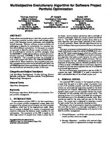
[2 57 15 43 14 44 38 86 16 61 17 84 45 8 46 36 49 64 19 47 48 82 7 52 18 83 60 5 91 100 13 58] [89 6 94 95 97 92 59 96 99 93 85 98 37 42 87 53] RC1 - 02 : [42 61 81 90] [95 85 63 76 51 84 56 66] [69 88 53 55 100 70] [94 31 29 27 26 89 91 80] [39 36 44 40 38 41 43 35 37 72] [82 11 15 16 9 10 13 17 12] [65 99 52 57 74 77 83] [64 86 87 59 97 75 58] [2 45 8 7 6 46 4 5 3 1] [48 21 23 18 19 22 49 20 24 25] [50 33 28 30 32 34 93 96] [14 47 73 79 78 60 98] [92 62 67 71 54 68] RC1 - 07 : [65 83 58 75 77 25 23 24] [90 61 81 54 96] [82 99 52 57 86 59 87 97 74] [42 44 39 38 36 35 37 40 43 41] [95 84 85 63 51 76 89 56 91] [72 71 93 94 67 50 92 80] [88 2 6 7 8 5 3 1 45 60 55] [12 14 47 17 16 15 11 13 9 10] [62 31 29 27 26 28 30 34 32 33] [69 98 53 78 73 79 46 4 100 70 68] [64 22 19 18 21 48 49 20 66] RC2 - 07 : [92 95 67 62 33 30 28 29 31 71 72 42 44 40 38 39 41 61 81 90 94 96 93 50 34 27 26 32 89 56 91 80] [82 11 15 16 47 14 12 73 79 7 6 2 8 5 45 46 4 3 1 43 36 35 37 54] [69 98 88 53 99 52 86 75 59 87 74 57 22 20 49 48 24 66]


147

[65 83 64 51 84 85 63 76 21 18 19 23 25 77 58 97 13 9 10 17 78 60 55 100 70 68]

Solution for RC2−07 : Black dots indicate 100 customer sites; the depot is represented by a black rectangle near the centre of map and routes are identified with different line styles. References 1. H.F. Dias Alexandre and A. de Vasconcelos Jõao, “Multiobjective genetic algorithms applied to solve optimization problems,” IEEE Transactions on Magnetic, vol. 38, no. 2, pp. 1133–1136, 2002. 2. T.Bäck, Evolutionary Algorithms in Theory and Practice, Oxford University Press: New York, 1996. 3. T.P. Bagchi, Multiobjective Scheduling by Genetic Algorithms, Kluwer Academic Publishers:Boston 1999. 4. J.F. Bard, G. Kontoravdis, and G. Yu, “A branch-and-cut procedure for the vehicle routing problem with time windows,” Transportation Science, vol. 36, no. 2, pp. 250–269, 2002. 5. J.E. Beasley and N. Christofides, “Vehicle routing with a sparse feasibility graph,” European Journal of Operational Research, vol. 98, no. 3, pp. 499–511, 1997. 6. P. Ben, R.C. Rankin, A. Cumming, and T.C. Fogarty, “Timetabling the classes of an entire university with an evolutionary algorithm,” Parallel Problem Solving From Nature V, Lecture Notes in Computer Science No. 1498, A. E. Eiben, T. Back, M. Schoenauer and H. Schwefel, Springer-Verlag:Amsterdam, 1998. 7. R. Bent and P. VanHentenryck, “A two-stage hybrid local search for the vehicle routing problem with time windows,” Computer Science Department, Brown University, RI, Technical Report CS-01–06, Sept. 2001. 8. J. Berger, M. Barkaoui, and O. Bräysy, “A parallel hybrid genetic algorithm for the vehicle routing problem with time windows,” Defense Research Establishment Valcartier, Canada, Working Paper, 2001. 9. D. Bertsimas and D. Simchi-Levi, “A new generation of vehicle routing research: robust algorithms, addressing uncertainty,” Operations Research, vol. 44, no. 2, pp. 286–304, 1993.

148

TAN, CHEW AND LEE

10. J.L. Blanton Jr. and R.L. Wainwright, “Multiple vehicles routing with time and capacity constraints using genetic algorithms,” Fifth International Conference on Genetic Algorithms, 1993, pp. 452–459. 11. O. Bräysy, “A reactive variable neighborhood search algorithm for the vehicle routing problem with time windows,” INFORMS Journal on Computing, vol. 15, no. 4, 2003. 12. O. Bräysy and M. Gendreau, “Genetic algorithms for the vehicle routing problem with time windows,” SINTEF Applied Mathematics, Department of Optimisation, Oslo, Norway, Internal Report STF42 A01021, 2001. 13. O. Bräysy and M. Gendreau, “Tabu search heuristics for the vehicle routing problem with time windows,” SINTEF Applied Mathematics, Department of Optimisation, Oslo, Norway, Internal Report STF42 A01022, 2001. 14. A.V. Breedam, “Comparing descent heuristic and metaheuristic for the vehicle routing problem,” Computer & Operations Research, vol. 28, no. 4, pp. 289–315, 2001. 15. E.K. Burke and J.P. Newall, “A multi-stage evolutionary algorithm for the timetable problem,” IEEE Transactions on Evolutionary Computation, vol. 3, no. 1, pp. 63–74, 1999. 16. Y. Caseau and F. Laburthe, “Heuristics for large constrained vehicle routing problems,” Journal of Heuristics, vol. 5, no. 3, pp. 281–303, 1999. 17. J.M. Chambers, W.S. Cleveland, B. Kleiner, and P.A. Turkey, Graphical Methods for Data Analysis, Wadsworth:Belmont, CA, 1983. 18. W. Chavalitwongse, D. Kim, and P.M. Pardalos, “GRASP with a new local search scheme for vehicle routing problems with time windows,” Journal of Combinatorial Optimization, vol. 7, no. 2, pp. 179–207, 2003. 19. C.L. Chen, R.V. Neppalli, and N. Aljabel, “Genetic algorithms applied to the continuous flowshop problem,” Computers and Industrial Engineering, vol. 30, no. 4, pp. 919–929, 1996. 20. W.C. Chiang and R.A. Russel, “Simulated annealing metaheuristic for the vehicle routing problem with time windows,” Annals of Operations Research, vol. 63, pp. 3–27, 1996. 21. W.C. Chiang and R.A. Ruseel, “A reactive tabu search metaheuristics for the vehicle routing problem with time windows,” INFORMS Journal on Computing, vol. 9, pp. 417–430, 1997. 23. N. Christofides, A. Mingozzi and P. Toth, “Exact algorithms for the vehicle routing problem based on spanning tree and shortest path relaxations,” Math. Programming, vol. 20, no. 3, pp. 255–282, 1981. 23. C.A. Coello Coello, “A comprehensive survey of evolutionary-based multiobjective optimization techniques,” Knowledge and Information Systems, vol. 1, no. 3, pp. 269–308, 1999. 24. C.A. Coello Coello, D.A. VanVeldhuizen, and G.B. Lamont, Evolutionary Algorithms for Solving Multi-Objective Problems, Kluwer Academic/Plenum Publishers, 2002. 25. W. Cook and J.L. Rich, “A parallel cutting plan algorithm for the vehicle routing problem with time windows,” Computational and Applied Mathematics Department, Rice University, Houston, TX, Technical Report, 1999. 26. J.F. Cordeau, M. Gendreau, G. Laporte, J.Y. Potvin, and F. Semet, “A guide to vehicle routing heuristics,” Journal of the Operational Research Society, vol. 53, no. 5, pp. 512–522, 2002. 27. J.-F. Cordeau, G. Laporte, and A. Mercier, “A unified tabu search heuristic for vehicle routing problems with time windows,” Journal of the Operational Research Society, vol. 52, no. 8, pp. 928–936, 2001. 28. R. Cordone and R. Wolfler-Calvo, “A heuristic for the vehicle routing problem with time windows,” Journal of Heuristics, vol. 7, no. 2, pp. 107–129, 2001. 29. D. Cvetkovic and I.C. Parmee, “Preferences and their application in evolutionary multiobjective optimization,” IEEE Transactions on Evolutionary Computation, vol. 6, no. 1, pp. 42–57, 2002. 30. Z.J. Czech and P. Czarnas, “A parallel simulated annealing for the vehicle routing problem with time windows,” Proc. 10th Euromicro Workshop on Parallel, Distributed and Network-based Processing, Canary Islands, Spain, pp. 376–383, 2002. 31. B. De Backer, V. Furnon, P. Kilby, P. Prosser, and P. Shaw, “Solving vehicle routing problems using constraint programming and metaheuristics,” Journal of Heuristics, vol. 6, no. 4, pp. 501–523, 2002. 32. K. Deb, Multi-objective Optimization using Evolutionary Algorithms, John Wiley & Sons:London, 2001. 33. M. Desrochers, J. Desrosiers, and M. Solomon, “A new optimization algorithm for the vehicle routing problem with time windows,” Operational Research, vol. 40, no. 2, pp. 342–354, 1992. 34. J. Desrosier, Y. Dumas, M. Solomon, and F. Soumis, “Time constraint routing and scheduling,” Handbooks in Operations Research and Management Science 8: Network Routing, M. Ball , no. (ed.), Elsevier Science Publishers:Amsterdam, 1995, pp. 35–139.


149

35. U. Dorndorf and E. Pesch, “Evaluation based learning in a jobshop scheduling environment,” Computers and Operations Research, vol. 22, pp. 25–40, 1995. 36. W. Dullaert, G.K. Janssens, K. Sörensen, and B. Vernimmen, “New heuristics for the fleet size and mix vehicle routing problem with time windows,” Journal of the Operational Research Society, vol. 53, no. 11, pp. 1232–1238, 2002. 37. M.L. Fisher, “Vehicle routing,” in Handbooks in Operations Research and Management Science 8: Network Routing, M. Ball, (ed), Elsevier Science Publishers:Amsterdam, 1995, pp. 1–33. 38. C.M. Fonseca, Multiobjective Genetic Algorithms with Application to Control Engineering Problems, Dept. Automatic Control and Systems Eng., University of Sheffield, Sheffield, UK, Ph.D. Thesis, 1995. 39. C.M. Fonseca and P.J. Fleming, “Genetic algorithm for multiobjective optimization, formulation, discussion and generalization,” in Genetic Algorithms: Proceeding of the Fifth International Conference. Morgan Kaufmann:San Mateo, CA, pp. 416–423, 1993. 40. H. Gehring and J. Homberger, “A parallel two phase metaheuristic for routing problems with time windows,” Asia-Pacific Journal of Operation Research, vol. 18, no. 1, pp. 35–47, 2001. 41. H. Gehring and J. Homberger, “Parallelization of a two-phase metaheuristic for routing problems with time windows,” Journal of Heuristics, vol. 3, no. 8, pp. 251–276, 2002. 42. M. Gendreau, G. Laporte, and J.Y. Potvin, “Metaheuristics for the vehicle routing problem,” University of Montreal, Canada, Les Cahiers du GERAD G-98-52, 1999. 43. A. Gezdur and M. Türkay, “MILP solution to the vehicle routing problem with time windows and discrete vehicle capacities,” XXIII National Operations Research and Industrial Engineering Congress, Istanbul, Turkey, July 2002. 44. D.E. Goldberg and R. Lingle, “Alleles, loci and the traveling salesman problem,” First International Conference on Genetic Algorithms. Lawrence Erlbaum:Hillsdale, NJ, 1985, pp. 154–159. 45. B.L. Golden and A.A. Assad, Vehicle Routing: Methods and Studies, North-Holland:Amsterdam 1988. 46. J.J. Grefenstette, R. Gopal, B. Rosmaita, and D. VanGucht, “Genetic algorithms for the traveling salesman problem,” First International. Conf. Genetic Algorithms and Their Applications, pp. 160–168, 1985. 47. W.K. Ho, H.J. Chin, and A. Lim, “A hybrid search algorithm for the vehicle routing problem with time windows,” International Journal on Artificial Intelligence Tools, vol. 10, pp. 431–449, 2001. 48. J. Homberger and H. Gehring, “Two evolutionary metaheuristic for the vehicle routing problem with time windows,” INFOR, vol. 37, no. 1, pp. 297–318, 1999. 49. G. Ioannou, M. Kritikos, and G. Prastacos, “A greedy look ahead heuristic for the vehicle routing problem with time windows,” Journal of the Operational Research Society, vol. 52, no. 5, pp. 523–537, 2001. 50. H. Ishibashi, H. Aguirre, K. Tanaka, and T. Sugimura, “Multi-objective optimization with improved genetic algorithm,” IEEE International Conference on Systems, Man, and Cybernetics (SMC2000), Nashville, pp. 3852–3857, 2000. 51. A. Jaszkiewicz, “Multiple objective metaheuristic algorithms for combinatorial optimization,” Poznań University of Technology, Poznan, Habilitation thesis 360, 2001. 52. A. Jaszkiewicz, “Genetic local search for multiple objective combinatorial optimization,” Institute of Computing Science, Poznań University of Technology, Research Report RA-014/98, 1998. 53. N. Jozefowiez, F. Semet, and E. Talbi, “Parallel and hybrid models for multi-objective optimization: application to the vehicle routing problem,” Parallel Problem Solving from Nature, Lecture Notes in Computer Science, Springer-Verlag:New York, 2002, pp. 271–282. 54. S. Jung and B.R. Moon, “A hybrid genetic algorithm for the vehicle routing problem with time windows,” The Genetic And Evolutionary Computation Conference, Morgan Kaufmann Publishers:San Francisco, 2002, pp 1309–1316. 55. B. Kallehauge, J. Larsen and O.B.G. Madsen, “Lagrangean duality applied on vehicle routing with time windows,” IMM, Technical University of Denmark, Technical Report IMM-TR-2001–9, 2001. 56. P.J. Kilby, P. Prosser, and P. Shaw, “Guided local search for the vehicle routing problem with time windows,” in Meta Heuristics: Advances and Trends in Local Search Paradigms for Optimisation. Kluwer Academic Publishers, 1999, pp. 473–486. 57. P.J. Kilby, P. Prosser, and P. Shaw, “A comparison of traditional and constraint-based heuristic methods on vehicle routing problems with side constraints,” Journal of Constraints, vol. 5, no. 4, pp. 389–414, 2000.

150

TAN, CHEW AND LEE

58. J.D. Knowles and D.W. Corne, “Approximating the nondominated front using Pareto archived evolutionary strategy,” Evolutionary Computation, vol. 8, no. 2, pp. 149–172, 2000. 59. N. Kohl, J. Desrosiers, O.B.G. Madsen, M.M. Solomon, and F. Soumis, “2 path cuts for the vehicle routing problem with time windows,” Transportation Science, vol. 33, no. 1, pp. 101–116, 1999. 60. G. Laporte, “The vehicle routing problem: An overview of exact and approximate algorithms,” Europe Journal of Operational Research, vol. 59, no. 3, pp. 345–358, 1992. 61. G. Laporte, M. Gendreau, J.Y. Potvin, and F. Semet, “Classical and modern heuristics for the vehicle routing problem,” International Transaction in Operational Research, vol. 7, pp. 285–300, 2000. 62. H.C. Lau, Y.F. Lim and Q.Z. Liu, “Diversification of Search Neighborhood via Constraint-Based Local Search and Its Applications to VRPTW,” 3rd International Workshop on Integration of AI and OR Techniques (CP-AI-OR), Kent, United Kingdom, pp. 1–15, 2001. 63. H.C. Lau, M. Sim and K.M. Teo, “Vehicle routing problem with time windows and a limited number of vehicles,” European Journal of Operational Research, vol. 148, no. 3, pp. 559–569, 2003. 64. L.H. Lee, K.C. Tan, K. Ou, and Y.H. Chew, “Vehicle Capacity Planning System (VCPS): A case study on vehicle routing problem with time windows,” IEEE Transactions on Systems, Man and Cybernetics: Part A (Systems and Humans), vol. 33, no. 2, pp. 169–178, 2003. 65. H. Li and A. Lim, “Local search with annealing-like restarts to solve the vehicle routing problem with time windows,” ACM Symposium on Applied Computing (SAC 2002), pp. 560–565, 2002. 66. S. Lin, “Computer Solutions for Traveling Salesman Problem,” Bell System Technical Journal, vol. 44, pp. 2245–2269, 1965. 67. S.J. Louis, X. Yin, and Z.Y. Yuan, “Multiple vehicle routing with time windows using genetic algorithms,” Proceedings of the Congress on Evolutionary Computation, pp. 1804–1808, 1999. 68. Z. Michalewicz, D.B. Fogel, and A. Michaelewica, How to Solve It: Modern Heuristics, Springer-Verlag, 1999. 69. T. Murata and H. Ishibuchi, “Performance evaluation of genetic algorithms for flow shop scheduling problems,” Computers and Industrial Engineering, vol. 30, no. 4, pp. 1061–1071, 1996. 70. I.M. Oliver, D.J. Smith, and J.R.C. Holland, “A study of permutation crossover operators on the traveling salesman problem,” in Proceedings of The Second ICGA, Lawrence Erlbaum Associates:New Jersey, 1987 pp. 224–230. 71. I.H. Osman and N. Christofides, “Simulated annealing and descent algorithms for capacitated clustering problem,” Imperial College, University of London, Research Report, 1989. 72. L.F. Paquete and C.M. Fonseca, “A study of examination timetabling with multiobjective evolutionary algorithms,” Metaheuristics International Conference, Porto:Portugal, 2001. 73. M. Pinaki and M.R. Elizabeth, Genetic Algorithms for VLSI Design, Layout & Test Automation, Prentice hall:New Jersey, 1999. 74. J.Y. Potvin, T. Kervahut, B. Garcia, and J.M. Rousseau, “A Tabu search for the vehicle routing problem with time window,” Centre de Recherche sur les Transports, University de Montreal, Canada, Technical Report CRT-855, 1993. 75. J.Y. Potvin, T. Kervahut, B. Garcia, and Rousseau J.M. Garcia, “The vehicle routing problem with time windows—part I: Tabu search,” INFORMS Journal on Computing, vol. 8, no. 2, pp. 158–164, 1996. 76. J.Y. Potvin and S. Bengio, “The vehicle routing problem with time windows—part II: genetic search,” INFORMS Journal on Computing, vol. 8, no. 2, pp. 165–172, 1996. 77. P.M.R. Prinetoo and M.S. Reorda, “Hybrid genetic algorithms for the traveling salesman problem,” Fifth International Conference on Genetic Algorithms, pp. 559–566, 1993. 78. C. Rego, “Node ejection chains for the vehicle routing problem: sequential and parallel algorithms,” Parallel Computing, vol. 27, no. 3, pp. 201–222, 2001. 79. Y. Rochat and E.D. Tailard, “Probabilistic diversification and intensification in local search for vehicle routing problem,” Journal of Heuristic, vol. 1, no. 1, pp. 147–167, 1995. 80. L.M. Rousseau, M. Gendreau, and G. Pesant, “Using constraint-based operators to solve the vehicle routing with time windows,” Journal of Heuristics, vol. 8, no. 1, pp. 43–58, 2002. 81. M.W.P. Savelsbergh, “Local Search for routing problems with time windows,” Annals of Operations Research, vol. 4, pp. 285–305, 1985. 82. J. Schulze and T. Fahle, “A parallel algorithm for the vehicle routing problem with time window constraints,” Annals of Operations Research, vol. 86, pp. 585–607, 1999.


151

83. P. Shaw, “Using constraint programming and local search methods to solve vehicle routing problems,” Principles and Practice of Constraint Programming—CP98, Lecture Notes in Computer Science, M. Maher and J.-F. Puget (eds), Springer-Verlag:New York, 1998, pp. 417–431. 84. M.M. Solomon, “Algorithms for vehicle routing and scheduling problem with time window constraints,” Operations Research, vol. 35, no. 2, pp. 254–265, 1987. 85. E. Taillard, P. Badeau, M. Gendreau, F. Guertin, and J.Y. Potvin, “A Tabu search heuristic for the vehicle routing problem with soft time windows,” Transportation Science, vol. 31, no. 2, pp. 170–186, 1997. 86. K.C. Tan, E.F. Khor, J. Cai, C.M. Heng, and T.H. Lee, “Automating the drug scheduling of cancer chemotherapy via evolutionary computation,” Artificial Intelligence in Medicine, vol. 25, pp. 169–185, 2002. 87. K.C. Tan, T.H. Lee, and E.F. Khor, “Evolutionary algorithm with dynamic population size and local exploration for multiobjective optimization,” IEEE Transactions on Evolutionary Computation, vol. 5, no. 6, pp. 565–588, 2001. 88. K.C. Tan, L.H. Lee, and K. Ou, “Hybrid genetic algorithms in solving vehicle routing problems with time window constraints,” Asia-Pacific Journal of Operational Research, vol. 18, no. 1, pp. 121–130, 2001. 89. K.C. Tan, L.H. Lee, and K. Ou, “Artificial intelligence techniques in solving vehicle routing problems with time window constraints,” Engineering Applications of Artificial Intelligence, vol. 14, pp. 825–837, 2001. 90. K.C. Tan, T.H. Lee, K. Ou, and L.H. Lee, “A messy genetic algorithm for the vehicle routing problem with time window constraints,” IEEE Congress on Evolutionary Computation, pp. 679–686, 2001. 91. K.C. Tan, L.H. Lee, Q.L. Zhu, and K. Ou, “Heuristic methods for vehicle routing problem with time windows,” Artificial Intelligence in Engineering, vol. 15, no. 3, pp. 281–295, 2001. 92. J. Tavares, F.B. Pereira, P. Machado, and E. Costa, “On the influence of GVR in vehicle routing,” ACM Symposium on Applied Computing (SAC 2003), Florida, USA, March, 2003. 93. S.R. Thangiah, “An adaptive clustering method using a geometric shape for vehicle routing problems with time windows,” Sixth International Conference on Genetics Algorithm, vol. 1, pp. 452–459, 1995. 94. S.R. Thangiah, I.H. Osman, and T. Sun, “Hybrid genetic algorithm, simulated annealing and Tabu search methods for vehicle routing problems with time windows,” Computer Science Department, Slippery Rock University, Technical Report SRU CpSc-TR-94-27, 1994. 95. P. Toth and D. Vigo, The Vehicle Routing Problem, SIAM:Philadelphia, 2002. 96. D. Van Veldhuizen and G.B. Lamont, “Multiobjective evolutionary algorithm research: a history and analysis,” Department of Electrical and Computer Engineering, Air Force Institute of Technology, Ohio, Technical Report TR-98-03, 1998. 97. D. Van Veldhuizen and G.B. Lamont, “Multiobjective evolutionary algorithms: analyzing the state-of-art,” Evolutionary Computation, vol. 8, no. 2, pp. 125–147, 2000. 98. D. Whitley, T. Starkweather, and D. Fuquay, “Scheduling problems and traveling salesmen: The genetic edge recombination operator,” Third International Conference on Genetic Algorithms, San Mateo, CA, 1989, pp. 133–140. 99. P. Yellow, “A computational modification to the saving method of vehicle scheduling,” Operational Research Quart., vol. 21, no. 2, pp. 281–283, 1970. 100. J. Czech Zbigniew and C. Piotr, “Parallel simulated annealing for the vehicle routing problem with time windows,” Silesia University of Technology, Technical report, 2001. 101. E. Zitzler and L. Thiele, “Multiobjective evolutionary algorithms: A comparative case study and the strength Pareto approach,” IEEE Transactions on Evolutionary Computation, vol. 3, no. 4, pp. 257–271, 1999.