Environmental Fluid Mechanics 3: 305–329, 2003. © 2003 Kluwer Academic Publishers. Printed in the Netherlands.
305
A Large-Eddy Simulation Study of the Convective Boundary Layer over Philadelphia during the 1999 Summer NE-OPS Campaign ANANTHARAMAN CHANDRASEKARa, C. RUSSELL PHILBRICKb, RICHARD CLARKc , BRUCE DODDRIDGEd and PANOS GEORGOPOULOSa,∗ a Environmental & Occupational Health Sciences Institute, NJ, U.S.A. b Department of Electrical Engineering, Pennsylvania State University, PA, U.S.A. c Department of Earth Sciences, Millersville University, Millersville, PA, U.S.A. d Department of Meteorology, University of Maryland, College Park, MD, U.S.A.
Received 5 August 2002; accepted in revised form 6 February 2003 Abstract. This study presents a large-eddy simulation (LES) study of the convective boundary layer on August 1, 1999 over Philadelphia, PA during a summer ozone episode. The study is an evaluation of the Colorado State University’s Regional Atmospheric Modeling System Version 4.3 (RAMS4.3) with the LES option using Northeast Oxidant and Particulate Study (NE-OPS) data. Simulations were performed with different imposed sensible heat fluxes at the ground surface. The model was initialized with the atmospheric sounding data collected at Philadelphia at 1230 UTC and model integrations continued till 2130 UTC. The resulting mean profiles of temperature and humidity obtained from the LES model were compared with atmospheric soundings, tethered balloon and aircraft data collected during the NE-OPS 1999 field campaign. Also the model-derived vertical profiles of virtual temperature were compared with NE-OPS Radio Acoustic Sounder System (RASS) data while the humidity profiles were compared with NE-OPS lidar data. The comparison of the radiosonde data with the LES model predictions suggests that the growth of the mixing layer is reasonably well simulated by the model. Overall, the agreement of temperature predictions of the LES model with the radiosonde observations is good. The model appears to underestimate humidity values for the case of higher imposed sensible heat flux. However, the humidity values in the mixing layer agree quite well with radiosonde observations for the case of lower imposed sensible heat flux. The modelpredicted temperature and humidity profiles are in reasonable agreement with the tethered balloon data except for some small overestimation of temperature at lower layers and some underestimation of humidity values. However, the humidity profiles as simulated by the model agree quite well with the tethered balloon data for the case of lower imposed sensible heat flux. The model-predicted virtual temperature profile is also in better agreement with RASS data for the case of lower imposed sensible heat flux. The model-predicted temperature profile further agrees quite well with aircraft data for the case of lower imposed heat flux. However, the relative humidity values predicted by the model are lower compared with the aircraft data. The model-predicted humidity profiles are only in partial agreement with the lidar data. The results of this study suggest that the explicitly resolved energetic eddies seem to provide the correct forcing necessary to produce good agreement with observations for the case of an imposed sensible heat flux of 0.1 K m s−1 at the surface. Key words: aircraft measurements, LES, lidar, NE-OPS, radiosonde, RAMS, RASS, tethered balloon ∗ Corresponding author, E-mail:
[email protected]
306
ANANTHARAMAN CHANDRASEKAR ET AL.
1. Introduction 1.1. RATIONALE There is an ever increasing need to enhance our understanding of and quantify the role of turbulence in atmospheric planetary boundary layer (PBL) processes. Indeed, turbulence in the PBL plays a very central role in determining the transfer of heat, momentum and mass (including pollutants) between the earth surface and the atmospheric environment. Models which provide for explicit resolution of eddies in the PBL, such as large-eddy simulation (LES) models, can improve the characterization of phenomena of turbulent transport and mixing. Also, a better understanding of turbulence can lead to improved PBL models which in turn can contribute to more refined air quality models [1]. An important attribute for any LES model is the ability to correctly simulate the structure and characteristics of atmospheric turbulence in the PBL. Hence, there is a need to perform an evaluation of LES modeling with appropriate observations in order to understand the limitations as well as strengths of the LES approach and its implementation. It is also currently becoming recognized that point estimates of ambient pollutant concentrations, representing ensemble means of volume averages (over the computational cells of urban or regional models) cannot provide the information on subgrid variability that is needed in population exposures studies. Current efforts aim to provide probabilistic descriptions of local (neighborhood scale or census tract/block scale) air quality that incorporate both uncertainty and variability in ambient concentrations. Large-eddy simulations can in principle be used to fulfill this goal. Large-eddy simulations can also be valuable in studies of turbulent chemical interactions in the convective boundary layer (CBL). In a non-LES chemistry transport model study, due to the volume averaging of the turbulent medium, large scale eddies in the CBL can contribute to chemical structures which are at variance with reality. However, large-eddy simulation combined with chemistry can define appropriate averages and provide for uncertainties and fluctuations in concentration estimates. In a recent study, Ching et al. [2] examine the various issues involved in modeling particulate matter (PM) and air toxics concentration fields and their role in human exposure models. Ching et al. [2] produced gridded air quality fields over Philadelphia using the Models-3/Community Multiscale Air Quality (CMAQ) modeling system and compared with results obtained from turbulence induced concentration fluctuations using a large-eddy simulations technique as well as results obtained from dispersion of point, street and area sources from street canyon flows using a combination of computational fluid dynamics (CFD) and wind tunnel modeling techniques. This analysis, in fact indicated that the extent of the resolved scale spatial variability varies with each pollutant species. The North American Research Strategy for Tropospheric Ozone – Northeast – Oxidant and Particle Study (NARSTO-NE-OPS) [3] has developed meteorological and air quality databases utilizing a variety of advanced measurement platforms such as instrumented aircraft, wind profiler, Radio Acoustic Sounder System
LARGE-EDDY SIMULATION STUDY
307
(RASS), lidar, tethered balloon sondes and rawinsondes. In the present study an evaluation of the large-eddy simulation option of the Colorado State University’s Regional Atmospheric Modeling System (RAMS 4.3) in modeling a convective boundary layer over Philadelphia, PA is undertaken by comparing the RAMS-LES results with aircraft, lidar, tethered balloon, RASS and radiosonde observations during a 1999 summer ozone episode. 1.2. BACKGROUND Large-eddy simulation (LES) studies of the atmospheric planetary boundary layer (PBL) are being increasingly employed to characterize processes affected by turbulence. LES is a numerical modeling technique designed to explicitly resolve the more energetic eddies in the PBL. In LES studies, the unresolved (subgrid-scale) motions chiefly contribute to dissipation of resolved turbulent energy. Several LES models were developed [4–7] following the pioneering work by Deardorff [8]. Since LES studies resolve explicitly the energetic eddies in the PBL, the horizontal grid resolution utilized in these studies is typically of the order of 100 m. A majority of LES studies reported in the literature have dealt with convective boundary layer (CBL) over homogeneous land surface [6, 9–11]. However, there have been studies that focused on aspects of land surface heterogeneity [12–16]. Hadfield et al. [7, 17] utilized the LES option of the Colorado State University’s Regional Atmospheric Modeling System (RAMS) [18, 19] to study the impact of high amplitude surface heat flux patterns on the CBL and found that under no background wind conditions, the CBL was marginally affected by relatively large heat flux pattern. Young [20] compared the profiles of turbulence statistics obtained from aircraft observations and numerical studies in rolling and flat terrain. Young [20] found no significant difference in the turbulent structure from results obtained with a uniform terrain as well as results obtained with topographical features of the order of 100 m. However, other studies [12, 21] provide evidence of impact of land surface heterogeneity on the CBL. Avissar and Schmidt [15] investigated the effects of surface heterogeneities resulting from surface sensible heat fluxes with different means, amplitudes and wavelengths on the convective boundary layer, by utilizing the LES option of RAMS. Their results indicate that the impact of amplitude and wavelength of a heat wave is nonlinearly dependent upon the mean heating rate and that circulations resulting from surface heterogeneity are stronger when the amplitude and wavelength of the heat wave are larger. Avissar et al. [22] performed LES studies by utilizing RAMS to simulate the convective boundary layer on July 1, 1987 over the region of the First International Satellite Land Surface Climatology Project Field Experiment (FIFE). Avissar et al. [22] utilized in their simulation the diurnal variation of mean surface fluxes and their spatial variation obtained from the FIFE observational network and compared the model results with observed atmospheric soundings as well as with volume-imaging lidar picture. Their results indicated that the model performed quite well, with its
308
ANANTHARAMAN CHANDRASEKAR ET AL.
estimates being within 1 K and 1 g kg−1 of the observed atmospheric soundings. Gopalakrishnan et al. [16] utilized the LES option of RAMS to evaluate the scale at which topography starts to significantly affect the mean characteristics and structure of turbulence in the convective boundary layer. Their results indicated that topography had very little impact on the mean properties of the CBL at horizontal length scales of less than 5 km while there were some effects at larger horizontal scales. Large-eddy simulations of dispersion in the convective boundary layer [23, 24] as well as in the stable boundary layer [25, 26] have been performed in recent years. Gopalakrishnan and Avissar [23] utilized the LES option of RAMS to study the impacts of land surface heterogeneity on dispersion in the convective boundary layer and found that the surface heat flux heterogeneities tend to generate atmospheric circulations which impede vertical mixing and hence have a marked influence on particle dispersion in the CBL. Fast [27] studied the relative role of local and regional scale processes on ozone in Philadelphia for the period July 15–August 4, 1999 by utilizing a non-LES coupled meteorological and chemical modeling system, the PNNL Eulerian Gas and Aerosols Scalability Unified System (PEGASUS) [28]. RAMS is the meteorological component of PEGASUS with the latter utilizing four nested grids with horizontal resolutions of 48, 24, 8 and 4 km, respectively. The two innermost grids were centered over Philadelphia while the outermost grid encompassed the eastern United States and the remaining grid encompassed regions of north-central and north-eastern United States and southern Canada. The mesoscale model results were evaluated with radar wind profiler and radiosonde data while the chemical transport model results were evaluated with aircraft, ozonesonde and surface monitoring data. The results indicated little model bias in the simulated model wind speed as compared to the wind profilers but the simulated wind direction was more westerly by about 15 degrees. The mixing layer temperature and specific humidity simulations were within 1–2 K and 1– 2 g kg−1 of the corresponding observational values. Ding et al. [29, 30] performed large-eddy simulation of the atmospheric boundary layer using a new subgrid scale model for unstable, neutral, weakly and moderately stable cases and obtained satisfactory results using the new subgrid-scale model. More recent studies exist in the literature where the LES option of RAMS is utilized [31–37]. 1.3. A BRIEF OVERVIEW OF NARSTO - NE - OPS The North American Research Strategy for Tropospheric Ozone – Northeast – Oxidant and Particle Study (NARSTO-NE-OPS) is a multi institutional collaborative research program set up under EPA initiative, to improve current understanding of the underlying causes for the occurrence of high ozone concentrations and increased levels of fine particles in the north-eastern United States. Various advanced meteorological (aircraft [38], lidar [39], tethered balloon [40] and radar wind profiler/RASS sounder [3, 41]) and air chemistry (ground based particle/chemical
LARGE-EDDY SIMULATION STUDY
309
samples [3]) measurements were made at the NE-OPS site at the Baxter Water Treatment Plant, Philadelphia, PA (40.0764◦ N, 75.0119◦ W) during three field campaigns conducted during the summers of 1998, 1999 and 2001 [3]. During the 1999 campaign (June 28 to August 19) eight pollution episodes occurred over Philadelphia (July 3–5, July 8–10, July 16–21, July 23–24, July 27–August 1, August 7–8, August 11–13, August 15–17, 1999), all of them resulting in measurements of high ozone concentration over Philadelphia. Pennsylvania State University Radar wind profiler/RASS sounder and lidar were operated at the Baxter Water Treatment Plant NE-OPS primary site while the radiosondes were released at Philadelphia by the Pacific Northwest National Laboratory (PNNL). The University of Maryland aircraft [38] and the DOE–G1 aircraft by the Brookhaven National Laboratory were operated over a region extending six square miles around the NEOPS site at Baxter Water Treatment Plant, Philadelphia. Millersville University [40] performed tethered balloon measurements at the NE-OPS Baxter Water Treatment Plant site at Philadelphia. The present investigation is primarily focused on an ozone episode that took place on August 1, 1999 over the Philadelphia region. The temperature and humidity profiles obtained from the LES model are compared with the PNNL radiosonde, tethered balloon, aircraft and lidar observations while the virtual temperature profiles obtained from the model are compared with the RASS observations. 2. Description of the LES Option in RAMS 4.3 The LES model utilized in the present study is the Colorado State University’s Regional Atmospheric Modeling System (RAMS) version 4.3 [18, 19]. A detailed description of the LES option in RAMS is provided by Pielke et al. [42] and hence only a brief summary is presented here. The horizontal grid adopted for the various simulations consisted of 46 cells in the east-west (x) direction and 40 cells in the north-south (y) direction with a grid resolution of 125 m. Fifty layers in the vertical direction with vertical grid spacing ranging from 10 m near the ground surface and increasing up to a maximum of 125 m, with a vertical grid stretch rate of 1.1 was adopted for this study. The height of the highest model level considered in this study is 3898.5 m. The study utilized the 1.5 order-of-closure scheme proposed by Deardorff [43] for subgrid-scale turbulence. Momentum fluxes were calculated at the bottom boundary according to Louis [44] and the sensible heat flux was directly imposed at the bottom boundary. The land-processes scheme, the cloud microphysics scheme and the radiation schemes were deactivated [23]. Cyclic conditions for the lateral boundary were utilized. A rigid lid was employed as top boundary condition with a Rayleigh friction scheme applied to the seven top layers in the vertical direction. This type of boundary condition absorbs spurious gravity waves and reduces reflection from the upper part of the simulated domain and is normally utilized in studies such as these [23].
310
ANANTHARAMAN CHANDRASEKAR ET AL.
The LES model was initialized with the temperature and water vapor mixing ratio profiles observed at 1230 UTC on August 1, 1999 over the NE-OPS site at the Baxter Water Treatment Plant, Philadelphia. The hot weather conditions were prevalent over the North East U.S. during the ozone episode (July 27–August 1, 1999), with temperatures of 34.44 ◦ C reported on August 1 over the region. Broken high clouds were seen during the day with winds being predominantly westerly on August 1, 1999. A cold front finally crossed the region on August 2, 1999 ending the ozone episode. The temperature and moisture profiles were available from aircraft, RASS, tethered balloon, lidar and radiosonde during the NE-OPS campaign on August 1, 1999 and since this day also characterized typical midlatitude midsummer conditions, the above day was chosen for the simulation. Some previous studies have utilized theoretical profiles to initialize the LES model (e.g., [14, 15]) while other studies have utilized sounding profiles to initialize the model (e.g., [22, 23]). In this study we have opted for the sounding profiles to initialize the model. Also, in all the simulations the domain was heated by a mean, constant kinematic sensible heat flux of either 0.1 or 0.2 K m s−1 at the ground surface [23]. The convective scales resulting from these mean heating rates compare well with studies of Deardorff [10] and Lamb [45]. Usually in LES studies, the land processes are not activated and hence it was decided to deactivate the land processes scheme in this study. Also, observed sensible heat flux information at the ground surface was not available and so it was decided to impose a constant uniform sensible heat flux at the lower boundary. Since the objective of this study was to evaluate the LES option of RAMS with NE-OPS observations, it was decided to use the topography (DEM 30 sec) and land use data from the RAMS database. It should be noted that the above data are not available in scales of the order of 100 m; however, one can expect that this limitation is unlikely to critically impact model results. Model simulations were started at 1230 UTC and continued for 9 h till 2130 UTC with a time step of integration of 2 s. 3. Results and Discussion 3.1. COMPARISON OF LES - RAMS PREDICTIONS WITH NE - OPS OBSERVATIONS The number of LES studies has been steadily increasing in recent years due to the rapid development of faster affordable computing machines. However, there have not been many studies designed to evaluate the ability of LES to adequately simulate the structure and characteristics of turbulence in the PBL. The main reason for the limited number of LES evaluation studies has been the lack of appropriate observations. In fact, a comprehensive LES evaluation study requires 3-D observations of wind components, temperature and scalars in the PBL with very high resolution in both spatial and temporal scales [22]. The NE-OPS 1999 field campaign did provide advanced measurement platforms such as instrumented aircraft, wind profiler, RASS, lidar, tethered balloons and radiosondes thus facilitating the present attempt to evaluate the LES option of RAMS by comparing the mean pro-
LARGE-EDDY SIMULATION STUDY
311
files of temperature and moisture with aircraft, RASS, tethered balloon, lidar and radiosonde data. All heights noted in the following figures refer to height above mean sea level. 3.1.1. Comparison of LES-RAMS Predictions with Radiosonde Data Figures 1 and 2 show comparisons of RAMS-LES predictions of mean temperature and water vapor mixing ratio with PNNL radiosondes at Philadelphia for the case where the entire domain is heated by a mean constant kinematic sensible heat flux of 0.2 K m s−1 at the ground surface. While Figure 1 presents the comparison for August 1, 1999; 1430 UTC (top panels) and 1630 UTC (bottom panels), Figure 2 shows the comparison for the same day at 1900 UTC (top panels) and 2130 UTC (bottom panels). The temperature profiles, as seen from radiosonde observations at 1430 UTC, 1630 UTC and 1900 UTC, are characterized by inversions (increase of temperature with height) around 950 hPa, 900 hPa and 820 hPa, respectively. Also, the observed water vapor mixing ratio profiles, at the above mentioned times, reveal the presence of uniform humidity values extending to around 960 hPa at 1430 UTC, to 900 hPa at 1630 UTC and to 825 hPa at 1900 UTC, respectively. The above radiosonde observations suggest that the mixing layer steadily increases its vertical extent from around 950 hPa at 1430 UTC to around 825 hPa at 1900 UTC. The temperature predictions by the LES model (Figures 1 and 2) clearly show the presence of inversion at around 925 hPa at 1430 UTC and around 820 hPa at 1900 UTC. Also, the humidity predictions by the LES model (Figures 1 and 2) reveal the presence of uniform humidity values extending to 925 hPa at 1430 UTC, to 875 hPa at 1630 UTC and to 825 hPa at around 1900 UTC. The above model results suggest that the mixing layer does steadily increase from 1430 UTC to 1900 UTC as required by observations and the growth of the mixing layer is reasonably well simulated by the LES model. The grid cell size in the vertical direction for the LES model is 50 m around 950 hPa and 125 m around 875 hPa. Hence, even the best simulation of the mixing layer by the model will result in small differences of the order of 50 m in the mixing layer height as compared to observations. Also, it is clear from Figures 1 and 2 that the temperature predictions are robustly simulated by the LES model and the agreement with radiosonde observations is good. It is pertinent to note here that the model results are averaged over a grid cell and model timestep while the observations are primarily point measurements. However, the humidity predictions by the LES model appear to somewhat underestimate the observations, especially in the lower layers with the model showing a difference of 1–2 g kg−1 with observations. In order to study the sensitivity of the imposed constant sensible heat flux, LES simulations were performed with a different value of 0.1 K m s−1 for the kinematic sensible heat flux at the ground surface. Figures 3 and 4 show the comparison of RAMS-LES predictions of mean temperature and water vapor mixing ratio profiles with PNNL radiosondes at Philadelphia for the case when the entire domain is heated by a mean constant kinematic sensible heat flux of 0.1 K m s−1
312
ANANTHARAMAN CHANDRASEKAR ET AL.
Figure 1. Comparison of radiosonde observations with RAMS-LES predictions of mean profiles of temperature and water vapor mixing ratio for August 1, 1999; 1430 UTC (top panels) and 1630 UTC (bottom panels) at Philadelphia for a constant surface sensible heat flux of 0.2 K m s−1 .
LARGE-EDDY SIMULATION STUDY
313
Figure 2. Comparison of radiosonde observations with RAMS-LES predictions of mean profiles of temperature and water vapor mixing ratio for August 1, 1999; 1900 UTC (top panels) and 2130 UTC (bottom panels) at Philadelphia for a constant surface sensible heat flux of 0.2 K m s−1 .
314
ANANTHARAMAN CHANDRASEKAR ET AL.
Figure 3. Comparison of radiosonde observations with RAMS-LES predictions of mean profiles of temperature and water vapor mixing ratio for August 1, 1999; 1430 UTC (top panels) and 1630 UTC (bottom panels) at Philadelphia for a constant surface sensible heat flux of 0.1 K m s−1 .
LARGE-EDDY SIMULATION STUDY
315
Figure 4. Comparison of radiosonde observations with RAMS-LES predictions of mean profiles of temperature and water vapor mixing ratio for August 1, 1999; 1900 UTC (top panels) and 2130 UTC (bottom panels) at Philadelphia for a constant surface sensible heat flux of 0.1 K m s−1 .
316
ANANTHARAMAN CHANDRASEKAR ET AL.
at the ground surface. The above-mentioned figures present the comparisons for the same times as Figures 1 and 2; they clearly reveal that the decrease in the imposed sensible heat flux at the ground surface caused a decrease in the mixing layer height. This is understandable, since a decrease in the imposed sensible heat flux will result in reduced convective activity and contribute to reduced vertical mixing thus causing a decrease in the mixing layer height. However, the water vapor mixing ratio predictions by the LES model reveal a better agreement with observations as far as values in the mixing layer are concerned, with the model showing an increase of 0.5–1.0 g kg−1 as compared to Figures 1 and 2 in the mixing layer. The reason for the decrease of humidity values predicted by the LES model for the case of higher imposed sensible heat flux appears less straightforward. In the present study the LES option in RAMS was utilized assuming that water can exist in the vapor phase and that there is no condensation. Considering the above assumption, higher imposed sensible heat flux will cause greater convection and more vigorous vertical mixing with drier air aloft which can then contribute to lower values of humidity. Also, unlike Figures 1 and 2, the temperature predictions reveal that the temperature values in the mixing layer are lower than corresponding observations. In the present study, a horizontal homogeneous initialization of the LES model using the observed temperature and water vapor mixing ratio profile was performed. Since the soil and vegetation models were deactivated for the LES study and since actual soil moisture data were not utilized in the initialization, there is a possibility that the model may simulate lower humidity values close to the surface. A decrease in the imposed sensible heat flux will produce mixing layer depths of smaller vertical extent. Also, with the model simulating lower humidity values close to the surface, the above will result in moisture being vertically mixed over smaller vertical depths which may be responsible for the higher values of humidity in the lower troposphere. The situation for the higher imposed sensible heat flux will correspond to lower values of humidity since the moisture will be mixed vertically over a larger vertical depth. 3.1.2. Comparison of LES-RAMS Predictions with Tethered Balloon Data Figure 5 shows the comparison of RAMS-LES predictions of mean temperature and relative humidity with tethered balloon data at the NE-OPS Baxter Water Treatment Plant site, Philadelphia for the case where the entire domain is heated by a mean constant kinematic sensible heat flux of 0.2 K m s−1 at the ground surface. Figure 5 shows the comparison for August 1, 1999, at 1500 UTC (top panels) and 1600 UTC (bottom panels), respectively. Two tethered balloons (7 m3 and 100 m3 ) were utilized by Millersville University during the NE-OPS program. The small balloon which recorded meteorological variables was utilized in a series of ascent/descent soundings to an altitude of 300 m at a rate of approximately 0.15–0.2 m s−1 . Typically one vertical profile was obtained every 30 min with a vertical resolution of 1–3 m. While the LES model appears to reasonably simulate the mean temperature profile at 1600 UTC, the model appears to overestimate
LARGE-EDDY SIMULATION STUDY
317
Figure 5. Comparison of tethered balloon observations with RAMS-LES predictions of mean profiles of temperature and relative humidity for August 1, 1999; 1500 UTC (top panels) and 1600 UTC (bottom panels) at Philadelphia for a constant surface sensible heat flux of 0.2 K m s−1 .
318
ANANTHARAMAN CHANDRASEKAR ET AL.
the temperature values at 1500 UTC. The relative humidity predictions by the LES model appear to underestimate the observations, with the model showing a difference of 6–8% with observations. Figure 6 shows the comparison of RAMSLES predictions of mean temperature and relative humidity with tethered balloon data over Philadelphia for the case where the domain is heated by a mean constant kinematic sensible heat flux of 0.1 K m s−1 at the ground surface. Figure 6 provides the comparison for the same times as Figure 5. It is clear from Figure 6 that the relative humidity profile as simulated by the LES model is in very good agreement with the tethered balloon data for both times (1500 and 1600 UTC). The decrease of the model humidity value with increase of imposed sensible heat flux is evident again. Unlike Figure 5, the LES model predicts temperature values that are lower than the tethered balloon observations for the case of lower imposed sensible heat flux. 3.1.3. Comparison of RAMS-LES Predictions with RASS Data Figure 7 presents a comparison of RAMS-LES predictions of virtual temperature with RASS data obtained at the NE-OPS Baxter Water Treatment Plant site, Philadelphia for the case where the entire domain is heated by a mean constant kinematic sensible heat flux of 0.2 K m s−1 at the ground surface. Figure 7 shows the comparison for August 1, 1999; at 1500 and 1800 UTC (top panels) and at 1900 and 2000 UTC (bottom panels), respectively. While the virtual temperature prediction agrees with observations at times 1800 and 1900 UTC, the model appears to overestimate the virtual temperature values at times 1500 and 2000 UTC. Angevine et al. [46], while comparing the wind profiler and RASS measurements with 450 m tall tower measurements, observed that the virtual temperature as measured by RASS may only be accurate to about 0.5 ◦ C. Also Zhang et al. [47] discuss the uncertainties associated with the different measurement platforms and provide evidence (Figure 8 of their paper) of differences of 1–2 ◦ C in the virtual temperature profile between the aircraft, tethered balloon and RASS measurements during the NE-OPS campaign around July 17, 1999; 2000 UTC. Zhang et al. [47], while comparing the NE-OPS RASS measurements, to NE-OPS tower based measurements, found the mean bias and standard deviation of the biases to be about 1 ◦ C. Figure 8 shows the same information as Figure 7 except that the former is for the case when the entire domain is heated by a mean constant kinematic sensible heat flux of 0.1 K m s−1 at the ground surface. Due to the reduced value of the imposed sensible heat flux, the virtual temperature predicted by the LES model is lower than that presented in Figure 7. However, the agreement with the RASS virtual temperature data is much better for this case of lower imposed sensible heat flux value. The virtual temperature profile depends on both temperature and humidity values. With an increase of imposed sensible heat flux at the surface, an increase of model temperature and, as explained earlier, a decrease in the model humidity value are to be expected. However, the dependence of temperature on virtual temperature
LARGE-EDDY SIMULATION STUDY
319
Figure 6. Comparison of tethered balloon observations with RAMS-LES predictions of mean profiles of temperature and relative humidity for August 1, 1999; 1500 UTC (top panels) and 1600 UTC (bottom panels) at Philadelphia for a constant surface sensible heat flux of 0.1 K m s−1 .
320
ANANTHARAMAN CHANDRASEKAR ET AL.
Figure 7. Comparison of RASS observations with RAMS-LES predictions of mean profiles of virtual temperature for August 1, 1999; 15 and 18 UTC (top panels) and 1900 and 2000 UTC (bottom panels) at Philadelphia for a constant surface sensible heat flux of 0.2 K m s−1 .
LARGE-EDDY SIMULATION STUDY
321
is more, and this is reflected as an increase of virtual temperature values with an increase of imposed sensible heat flux at the surface. 3.1.4. Comparison of RAMS-LES Predictions with Aircraft Data Figure 9 shows the comparison of RAMS-LES predictions of mean temperature and relative humidity with aircraft measurements over Philadelphia on August 1, 1999; 1430 UTC, for the case where the entire domain is heated by a mean constant kinematic sensible heat flux of 0.2 K m s−1 (top panels) and for the case where the imposed sensible heat flux is 0.1 K m s−1 (bottom panels), at the ground surface. The relative humidity observation values, shown in Figure 9 are characterized by very high values (85% or above) with values occasionally reaching 100%. While the LES model appears to reasonably simulate the temperature, except for slight overestimation close to the ground for the case of higher imposed sensible heat flux, the model appears to underestimate the relative humidity values. However, the figures in the bottom panel reveal that the LES model agreement with the aircraft temperature data is quite good for the case of lower imposed sensible heat flux. Also, the relative humidity as predicted by the model in the lower layers assumes higher values for the case of lower imposed sensible heat flux. Despite the underestimation of the humidity values, Figure 9 shows that the model does appear to simulate well the trends in the structure of the humidity profile. 3.1.5. Comparison of RAMS-LES Predictions with Lidar Data Figure 10 presents the comparison of RAMS-LES predictions of mean water vapor mixing ratio with lidar data over Philadelphia on August 1, 1999; 1700 and 1800 UTC, for the case where the entire domain is heated by a mean constant kinematic sensible heat flux of 0.2 K m s−1 (top panels) and for the case where the imposed sensible heat flux value is 0.1 K m s−1 (bottom panels) at the ground surface. The comparisons with lidar data were restricted to humidity profiles, as no temperature data were collected on August 1, 1999. The water vapor mixing ratio observations, as seen in Figure 10, appear to increase with a height up to 500 m. The LES model is unable to successfully simulate the above feature. It should be noted that uncertainties exist among different measurement platforms. Figure 11 displays typical water vapor mixing ratio and temperature profiles on August 1, 1999; 1500 UTC. The water vapor mixing ratio profile utilizes data from aircraft, lidar, tethered balloon and radiosonde while the temperature profile utilizes data from aircraft, tethered balloon and radiosonde. While there is reasonable agreement for the temperature profile between the different measurement platforms, the same is not true for the humidity profile. For the latter, there is acceptable agreement only between the tethered balloon and radiosonde data. The aircraft data are acceptably close to the radiosonde data only at heights of 2000 m and above. Also, the aircraft water vapor mixing ratio data assume high values (6–8 g kg−1 higher) in the lower layers as compared to the radiosonde and tethered balloon data. It is to
322
ANANTHARAMAN CHANDRASEKAR ET AL.
Figure 8. Comparison of RASS observations with RAMS-LES predictions of mean profiles of virtual temperature for August 1, 1999; 1500 and 1800 UTC (top panels) and 1900 and 2000 UTC (bottom panels) at Philadelphia for a constant surface sensible heat flux of 0.1 K m s−1 .
LARGE-EDDY SIMULATION STUDY
323
Figure 9. Comparison of aircraft observations with RAMS-LES predictions of mean profiles of temperature and relative humidity for August 1, 1999; 1430 UTC at Philadelphia for a constant surface sensible heat flux of 0.2 K m s−1 (top panels) and for 0.1 K m s−1 (bottom panels).
324
ANANTHARAMAN CHANDRASEKAR ET AL.
Figure 10. Comparison of lidar observations with RAMS-LES predictions of mean profiles of water vapor mixing ratio for August 1, 1999; 1700 and 1800 UTC at Philadelphia for a constant surface sensible heat flux of 0.2 K m s−1 (top panels) and for 0.1 K m s−1 (bottom panels).
LARGE-EDDY SIMULATION STUDY
325
Figure 11. Comparison of observations from different platforms (aircraft, lidar, tethered balloon, sonde) on August 1, 1999; 1500 UTC for water vapor mixing ratio (top left panel) and for temperature (top right panel) at Philadelphia.
be noted that the aircraft spiraled over a region extending six square miles around the NE-OPS Baxter Water Treatment Plant site while the lidar, tethered balloon and radiosonde were set up exactly at the NE-OPS Baxter Water Treatment Plant location in Philadelphia. The lidar water vapor mixing ratio data is characterized by increasing values with height, a feature not seen in the data obtained on other measurement platforms. 4. Conclusions This study presented an evaluation of a RAMS large-eddy simulation of the convective boundary layer on August 1, 1999 over Philadelphia, PA during a summer ozone episode. Simulations were performed with two different imposed sensible heat fluxes at the ground surface. Comparisons of observations from different measurement platforms indicate that while there is acceptable agreement for the temperature values, the same is not true for the humidity values. The humidity values obtained from aircraft and lidar were found to depart from the radiosonde and tethered balloon data with the latter two being reasonably close to one another. The comparison of the radiosonde data with the LES model suggests that the growth of the mixing layer is reasonably well simulated by the model. Overall, the agreement
326
ANANTHARAMAN CHANDRASEKAR ET AL.
of temperature prediction of the LES model with the radiosonde observations is good. The model appears to underestimate the humidity values for the case of higher imposed sensible heat flux. However, the humidity values in the mixing layer agree quite well with radiosonde observations for the case of lower imposed sensible heat flux. The model-predicted temperature and humidity profiles are in reasonable agreement with the tethered balloon data except for some small overestimation of temperature at lower layers and some underestimation of the humidity values. However, the humidity profiles as simulated by the model agree quite well with the tethered balloon data for the case of lower imposed sensible heat flux. The model-predicted virtual temperature profile is in better agreement with RASS data for the case of lower imposed sensible heat flux. The model-predicted temperature profile agrees quite well with aircraft data for the case of lower imposed heat flux. However, the relative humidity values predicted by the model are lower compared with the aircraft data. The model-predicted humidity profiles are only in partial agreement with the lidar data. The decrease in humidity values with increase of the imposed sensible heat flux suggests that increased convection and vigorous mixing of dry air aloft may contribute to lower humidity values. Overall, the agreement of the humidity predictions of the LES model with observations is better for the case of lower imposed sensible heat flux while the agreement of the temperature predictions of the LES model with observations is good. The results of this study suggest that the explicitly resolved energetic eddies seem to provide the correct forcing necessary to produce good agreement with observation for the case of an imposed sensible heat flux of 0.1 K m s−1 at the surface. Acknowledgements The authors acknowledge the efforts of all the group members of the NARSTONE-OPS research campaign in collecting and maintaining data from the various advanced research platforms. The first author thanks Dr S.B. Roy for clarifications on the LES option in RAMS. The authors thank Dr Chris Doran and Dr Jerry Allwine of PNNL for providing the radiosonde data. Support for this work has been provided by the U.S. EPA funded NorthEast Oxidant and Particle Study (NE-OPS) University Consortium (EPA-826373); the U.S. EPA funded Center for Exposure and Risk Modeling (CERM) at EOHSI (EPAR-827033); and the State of New Jersey Department of Environmental Protection (NJDEP) funded Ozone Research Center (ORC) at EOHSI. References 1. 2.
Kallos, G., Kotroni, K., Lagouvardos, M. and Papadopoulos, A.: 1999, On the transport of air pollutants from Europe to North Africa, Geophys. Res. Lett. 25, 619–622. Ching, J., Lacser, A., Byun, D., J., H. and Ozkaynak, H.: 2001, Modeled PM and air toxics concentration fields to drive human exposure models. In: Eleventh Annual Meeting of the Society of Exposure Analysis, pp. 372, Charleston, SC.
LARGE-EDDY SIMULATION STUDY
3.
4. 5. 6. 7.
8. 9. 10. 11. 12. 13.
14. 15.
16.
17.
18.
19.
20. 21.
327
Philbrick, C.R., Ryan, W.F., Clark, R.D., Doddridge, B.G., Dickerson, R.R., Koutrakis, P., Allen, G., McDow, S.R., Rao, S.T., Hopke, P.K., Eatough, D.J., Dasgupta, P.K., Tollerud, D.J., Georgopoulos, P., Kleinman, L.I., Daum, P., Nunnermacker, L., Dennis, R., Schere, K., McClenny, W., Gaffney, J., Marley, N., Coulter, R., Fast, J., Doren, C. and Mueller, P.K.: 2002, Overview of the NARSTO-NE-OPS program. In: Proceedings of the Fourth Conference on Atmospheric Chemistry: Urban, Regional, and Global-Scale Impacts of Air Pollutants, pp. 107–114, American Meteorological Society, Orlando, FL. Moeng, C.H.: 1984, A large-eddy simulation model for the study of planetary boundary layer turbulence, J. Atmos. Sci. 41, 2052–2062. Mason, P.J.: 1988, Large-eddy simulations of convective atmospheric boundary layer, J. Atmos. Sci. 45, 1492–1516. Schmidt, H. and Schumann, U.: 1989, Coherent structure of the convective boundary layer derived from large-eddy simulations, J. Fluid Mech. 200, 511–562. Hadfield, M.G., Cotton, W.R. and Pielke, R.A.: 1991, Large-eddy simulations of thermally forced circulations in the convective boundary layer. Part I: Small scale circulation with zero wind, Boundary-Layer Meteorol. 57, 79–114. Deardorff, J.W.: 1972, Numerical investigation of neutral and unstable planetary boundary layers, J. Atmos. Sci. 29, 91–115. Moeng, C.H. and Wyngaard, J.C.: 1984, Statistics of conservative scalars in the convective boundary layer, J. Atmos. Sci. 41, 3161–3169. Deardorff, J.W.: 1974, Three-dimensional study of the height and mean structure of a heated planetary boundary layer, Boundary-Layer Meteorol. 7, 81–106. Moeng, C.H. and Wyngaard, J.C.: 1988, Spectral analysis of large-eddy simulations of the convective boundary layer, J. Atmos. Sci. 45, 3573–3587. Briggs, G.A.: 1988, Surface inhomogeneity effects on convective diffusion, Boundary-Layer Meteorol. 45, 117–135. Hechtel, L.M., Moeng, C.H. and Stull, R.B.: 1990, The effects of nonhomogeneous surface fluxes on the convective boundary layer: A case study using large-eddy simulation, J. Atmos. Sci. 47, 1721–1741. Walko, R.L., Cotton, W.R. and Pielke, R.A.: 1992, Large eddy simulations of the effects of hilly terrain on the convective boundary layer, Boundary-Layer Meteorol. 58, 133–150. Avissar, R. and Schmidt, T.: 1998, An evaluation of the scale at which ground-surface heat flux patchiness affects the convective boundary layer using large-eddy simulations, J. Atmos. Sci. 55, 2666–2689. Gopalakrishnan, S.G., Roy, S.B. and Avissar, R.: 2000, An evaluation of the scale at which topographical features affect the convective boundary layer using large-eddy simulations, J. Atmos. Sci. 57, 334–351. Hadfield, M.G., Cotton, W.R. and Pielke, R.A.: 1991, Large-eddy simulations of thermally forced circulations in the convective boundary layer. Part II: The effect of changes in wavelength and wind speed, Boundary-Layer Meteorol. 58, 307–327. Walko, R.L., Tremback, C.J. and Hertenstein, R.F.A.: 1995, RAMS – The Regional Atmospheric Modeling System, Version 3b, User’s Guide, ASTER Division, Mission Research Corporation, Fort Collins, CO. Walko, R.L. and Tremback, C.J.: 2001, RAMS – The Regional Atmospheric Modeling System, Version 4.3/4.4, Introduction to RAMS 4.3/4.4, ASTER Division, Mission Research Corporation, Fort Collins, CO. Young, G.S.: 1988, Turbulence structure of the convective boundary layer. Part II: Phoenix 78 aircraft observations of thermals and their environment, J. Atmos. Sci. 45, 727–735. Huynh, B.P., Coulman, C.E. and Turner, T.R.: 1990, Some turbulence characteristics of convectively mixed layers over rugged and homogeneous terrain, Boundary-Layer Meteorol. 51, 229–254.
328 22.
23. 24. 25. 26. 27.
28.
29.
30.
31.
32.
33. 34. 35.
36. 37. 38.
39.
40.
ANANTHARAMAN CHANDRASEKAR ET AL.
Avissar, R., Eloranta, E.W., Gurer, K. and Tripoli, G.J.: 1998, An evaluation of the large-eddy simulation option of the Regional Atmospheric Modeling System (RAMS) in simulating a convective boundary layer: A FIFE case study, J. Atmos. Sci. 55, 109–130. Gopalakrishnan, S.G. and Avissar, R.: 2000, An LES study of the impacts of land surface heterogeneity on dispersion in the convective boundary layer, J. Atmos. Sci. 57, 352–371. Cai, X.M.: 2000, Dispersion of a passive plume in an idealised urban convective boundary layer: A large-eddy simulation, Atmos. Environ. 34, 61–72. Kemp, J.R. and Thomson, D.J.: 1996, Dispersion in stable boundary layers using large-eddy simulation, Atmos. Environ. 30, 2911–2923. Sorbjan, Z. and Uliasz, M.: 1999, Large-eddy simulation of air pollution dispersion in the nocturnal cloud-topped atmospheric boundary layer, Boundary-Layer Meteorol. 91, 145–157. Fast, J.D.: 2002, The relative role of local and regional-scale processes on ozone in Philadelphia. In: Proceedings of the Fourth Conference on Atmospheric Chemistry: Urban, Regional, and Global-Scale Impacts of Air Pollutants, pp. 121–124, American Meteorological Society, Orlando, FL. Fast, J.D., Doran, J.C., Shaw, W.J., Coulter, R.L. and Martin, T.J.: 2000, The evolution of the boundary layer and its effect on air chemistry in the Phoenix area, J. Geophys. Res. 105, 22833–22848. Ding, F., Arya, S.P. and Lin, Y.L.: 2001, Large-eddy simulations of the atmospheric boundary layer using a new subgrid-scale model I. Slightly unstable and neutral cases, Environ. Fluid Mech. 1, 29–47. Ding, F., Arya, S.P. and Lin, Y.L.: 2001, Large-eddy simulations of the atmospheric boundary layer using a new subgrid-scale model II. Weakly and moderately stable cases, Environ. Fluid Mech. 1, 49–69. Ludwig, F.L., Street, R.L., Schneider, J.M. and Costigan, K.R.: 1996, Analysis of small-scale patterns of atmospheric motion in a sheared, convective boundary layer, J. Geophys. Res. 101, 9391–9411. Duda, D.P., Stephens, G.L., Stevens, B. and Cotton, W.R.: 1996, Effects of aerosol and horizontal inhomogeneity on the broadband albedo of marine stratus: Numerical simulations, J. Atmos. Sci. 53, 3757–3769. Eastman, J.L., Pielke, R.A. and McDonald, D.J.: 1998, Calibration of soil moisture for largeeddy simulations over the FIFE area, J. Atmos. Sci. 55, 1131–1140. Jiang, H.L. and Cotton, W.R.: 2000, Large eddy simulation of shallow cumulus convection during BOMEX: Sensitivity to microphysics and radiation, J. Atmos. Sci. 57, 582–594. Jiang, H.L., Fiengold, G., Cotton, W.R. and Duynkerke, P.G.: 2001, Large-eddy simulations of entrainment of cloud condensation nuclei into the Arctic boundary layer: May 18, 1998, FIRE/SHEBA case study, J. Geophys. Res. 106, 15113–15122. Cheng, W.Y.Y., Wu, T. and Cotton, W.R.: 2001, Large-eddy simulations of the 26 November 1991 FIRE II cirrus case, J. Atmos. Sci. 58, 1017–1034. Golaz, J.C., Jiang, H.L. and Cotton, W.R.: 2001, A large-eddy simulation study of cumulus clouds over land and sensitivity to soil moisture, Atm. Res. 59, 373–392. Doddridge, B.G.: 2000, An airborne study of chemistry and fine particles over the U.S. MidAtlantic region. In: Proceedings of the PM2000: Particulate Matter and Health Conference, pp. 4–5, Air and Waste Management Association, Charleston, SC. Li, G., Philbrick, C.R. and Allen, G.: 2002, Raman lidar measurements of airborne particulate matter. In: Proceedings of the Fourth Conference on Atmospheric Chemistry: Urban, Regional, and Global-Scale Impacts of Air Pollutants, pp. 135–139, American Meteorological Society, Orlando, FL. Clark, R.D., Philbrick, C.R. and Doddridge, B.G.: 2002, The effects of local and regional scale circulations on air pollutants during NARSTO-NEOPS 1999–2001. In: Proceedings of
LARGE-EDDY SIMULATION STUDY
41.
42.
43. 44. 45. 46.
47.
329
the Fourth Conference on Atmospheric Chemistry: Urban, Regional, and Global-Scale Impacts of Air Pollutants, pp. 125–132, American Meteorological Society, Orlando, FL. Philbrick, C.R. and Mulik, K.: 2000, Applications of Raman lidar to air quality measurements, In: Proceedings of the SPIE Conference on Laser Radar Technology and Applications V, Vol. 4035, pp. 22–33. Pielke, R.A., Cotton, W.R., Walko, R.L., Tremback, C.J., Lyons, W.A., Grasso, L.D., Nicholls, M.E., Moran, M.D., Wesley, D.A., Lee, T.J. and Copeland, J.H.: 1992, A comprehensive meteorological model system-RAMS, Meteorol. Atmos. Res. 49, 69–91. Deardorff, J.W.: 1980, Stratocumulus-capped mixed layers derived from a three-dimensional model, Boundary-Layer Meteorol. 18, 495–527. Louis, J.E.: 1979, A parametric model of vertical eddy fluxes in the atmosphere, BoundaryLayer Meteorol. 17, 187–202. Lamb, R.G.: 1978, A numerical simulation of dispersion from an elevated point source in the convective planetary boundary layer, Atmos. Environ. 12, 1297–1304. Angevine, W.M., Bakwin, P.S. and Davis, K.J.: 1998, Wind profiler and RASS measurements compared with measurements from a 450-m tall tower, J. Atmos. Oceanic Technol. 15, 818– 825. Zhang, K., Mao, H., Civerolo, K., Berman, S., Ku, J.Y., Rao, S.T., Doddridge, B.G., Philbrick, C.R. and Clark, R.D.: 2001, Numerical investigation of boundary-layer evolution and nocturnal low-level jets: Local versus non-local PBL schemes, Environ. Fluid Mech. 1, 171–208.