[10] W. Kruiskamp and D. Leenaerts, âDarwin: Cmos opamp synthesis by ... [11] M. Krasnicki, R. Phelps, Rob A. Rutenbar, and L. R. Carley, âMaelstrom: Effi-.
A Layout-aware Synthesis Methodology for RF Circuits P. Vancorenland, G. Van der Plas, M. Steyaert, G. Gielen and W. Sansen Katholieke Universiteit Leuven, Department of Electrical Engineering, ESAT MICAS Kasteelpark Arenberg 10, B-3001 Leuven-Heverlee, Belgium
{vanco,vdplas,steyaert,gielen,sansen}@esat.kuleuven.ac.be
In this paper a layout-aware RF synthesis methodology is presented. The methodology combines the power of a differential evolution algorithm with cost function response modeling and integrated layout generation to synthesize RF Circuits efficiently, taking into account all layout parasitics during the circuit optimization. The proposed approach has successfully been applied to the design of a high-performance downconverter mixer circuit, proving the effectiveness of the implemented design methodology.
1
Introduction
The ever expanding market for wireless data communication has recently given an enormous increase in the demand for smaller and cheaper radio-frequency integrated circuits (RF ICs). This demand is predicted to keep on growing in the foreseeable future. Presently most attention is paid to applications in the frequency range between 900 MHz and 5 GHz (like GSM, DECT, DCS-1800, wireless LAN, Bluetooth). Some common properties characterize the whole area of analog RF design. An extremely wide range in frequencies, combined with a very high dynamic range of the signals are typical difficulties for analog RF design. At GHz frequencies, all the parasitic elements of both the active and passive elements also come into play. The goal of an RF designer is to get a finished design that meets certain specifications at a minimal cost under severe time-to-market conditions. One way of achieving this is to employ optimization techniques for the circuit sizing while incorporating all layout parasitics. Analysis of RF circuits ranging from passive devices like integrated inductors to active circuits like LNAs, VCOs,. . . can be divided into two areas. On one side there are the simulators that will simulate the characteristics of the circuit, hence consuming a lot of CPU power [1], [2]. Using this approach to evaluate the RF circuit in the iteration loop of the optimization is impractical and time consuming. On the other side there are the models that approximate the system over a specific range of interest within a limited accuracy [3]. This alleviates the CPU problem in the course of an optimization, but has limited accuracy. In [4] an optimization algorithm is presented that uses the best of both sides. Most of the evaluations will be on an approximate model built on previous evaluations, but after an adaptive number of steps the approximation is corrected by evaluating the circuits again by simulation. This approach radically reduces optimization times for designs with very CPU consuming simulations while still keeping the desired accuracy. The algorithm builds, next to optimizing the circuit, a performance response model, in order to consecutively optimize on the circuit and on the model until a certain stop criterion is met. This optimization algorithm has been combined with a layout generation tool [5] to estimate accurately
layout parasitics during the optimization while still designing the RF circuits efficiently. In this paper the approach from [4] is extended. No layout estimates are used, instead the layout generation has been moved inside the optimization loop, improving the efficiency of the design process by removing a redesign loop from layout back to sizing. This approach has successfully been applied to the design of a low-power, lownoise mixer circuit. This paper is organized as follows. First the improved approach to RF circuit synthesis is described in section 2. In section 3 the layoutaware synthesis methodology is presented. In section 4 the example mixer architecture used to combine low noise, low power and highspeed performance is explained and its optimization is described in detail. Conclusions are drawn in section 5.
2 Layout-aware Analog Circuit Synthesis In [6] an overview was given of recent research progress in the analog synthesis domain. Typically, the task is split up in analog sizing (front-end) tools on the one hand and analog layout generation (back-end) on the other hand. This splitting up of the analog synthesis task is a de facto standard, since it is considered impractical or impossible to solve both problems simultaneously. However, when faced with RF design, the impact of layout parasitics on the circuit’s operation is often detrimental forcing the merger of these two steps. Thus during sizing synthesis at least an accurate estimate of the layout parasitics is required [5], [7], or the loop shown in Fig. 1 on the left will not converge. TRADITIONAL Specifications
Redesign loop
Abstract
PROPOSED Specifications Differential Evolution
Sizing Synthesis
Layout Generation
Layout
Layout Aware Synthesis
Equations Numerical Simulation Layout Generation
Layout
Figure 1.
Traditional approach of analog synthesis on the left, proposed layout-aware analog synthesis on the right
In this paper the sizing and layout generation have been merged into one optimization process (see Fig. 1 on the right), effectively removing the redesign loop from layout to sizing that exists in the traditional analog synthesis approach. To reach a practical application of this method, the power of the Differential Evolution (DE) optimizer [8] has been combined with accurate device-level simulation, a fast layout generation methodology and manually derived, accurate equations modeling the behavior of the mixer circuit. The different parts of this methodology will be described in the next sections.
3
Proposed Methodology
For a given circuit and target specifications, it is possible to define a cost function describing the cost or inversely the quality of the design. Generally speaking, the optimization problem can be described as: for given sets of parameters and cost functions: Pi ∈ [Pi,min Pi,max ]
i = 1..N
Cost j (P1 ..PN )
j = 1..M
Find the parameter set [P1opt ..PNopt ] satisfying min
∑
j=1..M
Cost j (P1 ..PN )
The strategy to obtain this parameter set [P1opt ..PNopt ] has to be both quick and accurate. A quick algorithm [9] may often end up in a local minimum of the cost function. Simulated Annealing is an algorithm that can guarantee to find the global optimum, but at moderate CPU times. Genetic Algorithms or “Simulated Evolutions” have recently become widely accepted as optimization routines for analog circuit design [10], [11] because of their ability to find a global optimum in a relatively short time. In this paper, a Genetic Algorithm called “Differential Evolution” (DE) [8] is used as optimization routine for this RF circuit optimization which is characterized by long evaluation times for each iteration.
3.1
Combined Evolutionary Algorithm
A genetic algorithm is an optimization algorithm that starts from a given population (or set of optimization parameters) and evaluates the fitness of its members (or inversely their cost) and then tries to increase that fitness (or decrease the cost) by selectively recombining its members, forming “children” for the next population. Only the “fittest” ones will survive from one population to another resulting in a hopefully better fit population (or better design solution). The routine that controls the whole optimization process, consists of three major subblocks as given in Fig. 2. At first a DE optimization strategy is started where a cost func-
Quality of fit high
low
Use fitted cost function N times
Use direct cost function (simulation) M times
Differential Evolution
Differential Evolution
Population
Fit Cost function
Figure 2. The major sub blocks of the optimization process based on “Differential Evolution” (DE)
tion is built out of circuit evaluations with a circuit level simulator. The evaluated points are stored and gradually the cost function is fitted within a radius around the optimal point. This is depicted in the right side loop of Fig. 2. When the fitted function corresponds well enough with newly simulated points, the optimization strategy evolves to the left side loop using the fitted function as cost function.
This function is evaluated over N times whereafter the optimization again returns to the right side loop. The radius δ around the optimum in which the cost function is fitted depends on the active step length of the algorithm. This length is determined by the distance between consecutive optimal parameter sets. Relating the radius δ to this length automatically ensures a contraction of the fitting space. It can clearly be seen that this algorithm has many advantages: • It uses the very fast and efficient “Differential Evolution” optimization strategy. • it is faster than a “Spice in the loop” approach since a major part of the cost function evaluations is done on a faster fitted model. • The use of a behavioral model to fit the cost function will generally generate a better fitting over a wider range compared to a polynomial approximation. • It is possible to cascade the algorithm with a non-stochastic algorithm like the Hooke and Jeeves algorithm [9] looking for the final optimum in a more greedy way, leading to even greater convergence speeds. • The algorithm is inherently parallel, making it very suitable for parallel optimizations, resulting in speed increases roughly equal to the level of parallellisation. The choice of an independent set of optimization parameters has a major influence on the speed of the algorithm. The set of parameters has to be mutually independent and as small as possible. It is best to select the ranges of the optimization parameters in such a way that the overall search space is minimized. It is for instance better to select the parameter set {P1 ,factor} (with P2 =P1 *factor) than {P1 ,P2 }, if it is possible on beforehand to say that P2 will have an optimal value roughly proportional to P1 . This is implemented in the example given in section 4.2.
3.2
Cost Function Fitting
The function the cost function is fitted to, directly has an impact on the speed and success of the algorithm. With increasing fitting error, the optimization on a fitted model will lead to an increasingly erroneous point, out of which the optimization of the objective function has to start, decreasing the possibility of a successful result. Since a circuit designer generally has some a-priori knowledge about a circuit in the form of “hand calculation” formulas, it is beneficiary to use these as the fitting function as is explained in section 4.1. In section 4 the equations used to model the circuit will be described in full detail. If no simple formulas are available, a multiquadrics [12] approximation is used. A systematic method for building a signomial and posynomial performance models is presented in [13]. The algorithm used for fitting the cost function is preferably a non-stochastic algorithm because of its greediness and speed. In the proposed methodology, the Hooke-Jeeves [9] algorithm is used. Experiments show a considerable speed gain compared to a genetic algorithm when used for fitting. When reasonable starting values for the fit are determined, based on the model formulas, a reasonable fast fitting process is achieved thus increasing considerably the efficiency of the optimizer in terms of number of circuit evaluations.
3.3
Layout Generation
Procedural module generators for device structures have been around as early as [14], [15]. Frequently occurring basic devices as for instance MOS transistors, resistors, capacitors, etc. or basic structures as for instance differential pairs, current mirrors, etc. are implemented using module generators. These module generators are either used manually or in an analog place and route environment [16],
[17]. This approach is however not usable when sizing and layout are combined in one optimization loop. In RF design the circuits are typically small, with a limited number of transistors. The requirements in contrast are even stronger than with “normal” analog design. The balanced mixer is a representative example in this respect. The circuit is double balanced: symmetrical, four identical, cross-coupled parts realize the requested behavior. Any deviation from this quadruple symmetry reduces the obtainable performance. Furthermore in the GHz range, all parasitics are important: resistance of wires, capacitive loading on wires, etc. Procedural generation can handle all the requirements. However creating module generators for every RF building block is tiresome unless the common operations are easily implemented: mirroring, copying, enlarging, . . . In [5] a layout generation method is proposed which has the requested functionality. The layout generator takes a template and manipulates it with simple, yet powerful operations to realize the complete circuit rapidly. This approach has been applied to the optimal design of a mixer circuit. Its template will be described in detail in the next section.
LO
M 3an
+
M lbn2
M lan2
M lan1
n1an M 2an
M lbn1
n1bn M1an
M 1bn
-
M2bn
LO
M 3bn
M lbp1
M lbp2
LO
M 3bp
-
M lap1
n1bp M2bp
n1ap M 1ap
Rin Outn
M lap2
M 1bp
M 2ap
LO
+
M 3ap
Rip -
RF
+
RF
4.1
Performance Models for Optimization
The models used to fit the cost function to are described below. They are based on manually derived equations. • Ibias The bias current and transconductance of the transistors can be given by: Ibias
=
gm
=
2 Vgst,M KP We f f 1 . . .(1 + λ.Vds ) 2 Le f f 1 + thetaVgst,M1 ∂Ibias ∂Vgs
The transistor size information is extracted from the layout geometry information. • IIP3 The input-referred third-order intermodulation intercept point is determined by the maximum current swing transistor M1 can tolerate. This current swing is inversely proportional to the value of the input resistor. The maximum tolerable swing is determined by the biasing condition of M1 . When the input resistance seen by Rin is low compared to the value of Rin , the IIP3 can be modeled as 2 IIP3 ∼ Rin2 ∗ Ibias ∗ α(Zin Rin ) 1
where α is a fitting factor depending on the input impedance. • gmconv The conversion transconductance determining the mixer gain, is the product of the inverse of the input resistances Rin as seen by a differential signal and the current mirroring efficiency to the output.
Outp
gmconv ∼ Figure 3. Schematic of the mixer circuit
4
Experimental Results for a Mixer Circuit
A fundamental building block in the analog part of a transceiver is the mixer. Linearity, dynamic range and power consumption are the most important specifications of this device. It is well-known that a mixer circuit is a hard to design component in these systems. This is why it was selected as a first candidate to be implemented with the proposed synthesis methodology. In this paper, an improved mixer architecture [18] is taken as example, since it uses circuit techniques to optimize the trade-off between these several specifications, making it an ideal candidate for inclusion in an optimization environment. The architecture of the mixer is shown in Fig. 3. The mixer is a double balanced structure with a resistive input. It uses cross coupling of the Ml transistors in order to achieve different impedance levels for different signals. The double balancing of the input structure will, in combination with these different impedance levels, provide a higher linearity and an inherently lower noise level. The voltage-to-current conversion is performed very linearly using resistors. Using a nowadays standard deep submicron CMOS technology the transistor ft is high enough to bias most of the transistors in the Moderate Inversion region, thereby reducing the power consumption while still achieving good frequency performance. This concludes the description of the mixer architecture. Next will be explained how this circuit was introduced in the synthesis methodology.
1 .ηmirror 2Rin
• Noise The total noise power density at the input of the mixer can be calculated. Relating this to the noise density of a 50Ω system gives the noise figure: � 2 � dvin, total NF = 10log10 kT ∗ 50 • f3dB The frequency performance is limited by the GBW of the feedback loop: g m1 GBW = Cn Cn = CGS1 +CGS3 + 2CDBl +CDB2 +Cinterconnect The transistor capacitances will scale with the sizes of the transistors. The interconnect capacitance is extracted from the layout as will be explained in section 4.2. Since the total capacitance on this node n1n determines the frequency performance of the mixer, it is clear that in order to get reliable GHz performance, the capacitance on this node has to be optimized as good as possible. Herefore it absolutely has to be integrated in the optimization loop as is done in or approach. • Zin Although it doesn’t directly influence the performance, the input impedance is an important parameter determining the linearity of the mixer and is given by: 1 Zin = gm2 .gm1 .(ro1 //rol )
4.2
Mixer Layout Template
The mixer layout is generated procedurally at each iteration of the optimization loop according the the following template. In Fig. 4
strips is selected as the reference value. The other number of strips are derived from this reference value: ]stripsM1,3 = ]stripsref ]stripsM2 = ]stripsref + ∆stripsM2
]stripsMl1,2 = ]stripsref + ∆stripsMl1,2
Mlbp1,2
M2bp
Together with the height of the active areas these determine the widths of all the transistors:
M1bn
WM1,3 = 2 heightM1,3 ]stripsM1,3
M3bp
M3bn
Mlan1,2
M1bp
Mlbn1,2
Mlap1,2 M3ap
M2an
M3an
M2bn
M1an
WM2 = 2 heightM2,l ]stripsM2
M2ap M1ap
Figure 4. Floorplan of complete mixer core, one quarter is high-
WMl1,2 = heightM2,l ]stripsMl1,2
lighted
the core of the mixer circuit is shown. The highlighted part is used 4 times in the double balanced mixer core. By generating a dense basic layout of this one-quarter structure and mirroring the result, the complete mixer core can easily be generated. The complete mixer layout is shown in Fig. 4. When the single-ended part is generated, only two mirroring commands are required to generate the complete mixer. The only remaining problem is to generate a dense, single-
The thus obtained independent parameters (heightM1,3 , heightM2,l , stripsref , ∆stripsM2 and ∆stripsMl1,2 ) are the optimization parameters varied by the DE algorithm. CF
CL
CF
CF
CF CA
CA
Figure 6.
Parasitic capacitance extraction: CA , CL and CF are technology parameters
height M1,3
M1
height M2,l
M2 copy/remove to change #strips M2 only
M3
stretch height M1,3
Ml1,2 copy/remove to change #strips M3 & Ml1,2
Figure 5. Mixer template ended mixer core as shown in Fig. 4. In Fig. 5 the template is shown that is used to generate the single-ended mixer core. The MOS transistors are drawn with minimal dimensions. All source and drain areas have been merged to reduce parasitics. Also all connections have been realized by abutment, if possible, and otherwise have been kept as short as possible. The transistor pair Ml1 and Ml2 has been interdigitated to have the best possible matching. Substrate and well straps are placed closely to all transistors, ensuring a clean back gate of the transistors. Indicated on the figure is the height of the active areas of transistors M1 and M3 , and the height of the active areas of transistors M2 and pair Ml1,2 . They can independently be modified as is shown on the figure for transistors M1 and M3 , by stretching the template vertically at the indicated lines. The number of strips of transistor M2 and both transistors M3 and Ml1,2 can be modified, by copying the greyed-out parts of the layout and pushing the not-selected parts out of the way. Extra selection boxes [5] are present in the actual template, making it possible to independently alter the number of strips of transistor pair M1 and M3 , transistor M2 and transistor pair Ml1,2 . It must be noted however that the most dense layout is obtained when the number of strips are approximately equal (as is the default of the template). In total there are thus five independent layout geometry parameters: heightM1,3 , heightM2,l , stripsM1,3 , stripsM2 and stripsMl1,2 . These allow the individual widths of the transistors to be varied independently. Since the most dense result (and thus the one with almost equally sized transistors) is typically the best, one of the number of transistor
The (lumped) parasitics of the transistors are calculated as follows: area of drain and source (ad, as), perimeters of drain and source (pd, ps), number of squares in drain and source (nrd, nrs). These are standard SPICE transistor parameters. The lumped extrinsic gate resistance (the wire connecting the gate strips) and intrinsic gate resistance (the resistance of the gate strips) are also extracted. The overlap and fringing capacitance of the metal1 and poly wires of the critical net n1 is calculated using a 2 1/2-D model of overlap, fringing and sidewall capacitance [19], as shown Fig. 6. These calculations are not an estimate as is usually the case; the obtained dimensions of the generated layout are used to calculate these values. The actual mirroring, copy and extraction calculations are approximately 100 lines of code (in a dedicated procedural layout language), of which the majority is taken up by the extraction calculations. In total this template evaluation takes less than 300 milliseconds of CPU time on a standard workstation. The obtained extracted netlist is passed back to the optimizer for the cost function optimization.
4.3
Practical Synthesis Result
The optimal design of the mixer circuit is now described. Measurement results have been included. The following specifications are used for the optimization problem, see Table I. Specification f3db gm (conversion gain) IIP3 NFDSB (noise figure) Supply Voltage Power Technology
Spec. Meas. > 3.4 3.4 > 2 2.1 > 0 2.3 < 20 20 = 2.7 2.7 MINIMIZE 0.0003 1P3M 0.35µ CMOS
Unit GHz mS dBm dB V W
Table I. Specified and measured performance summary From these specifications, the cost function can be calculated for an evaluated circuit as described in section 4.1.// The more degrees of freedom are used in an optimization strategy, the slower the opti-
mal point is found. Therefore the cost function was enhanced with some extra penalties that are not directly related to the performance parameters. This will help push the optimization process to a more favourable direction. • Input impedance. The input impedance seen by the input resistor Rin is not a direct performance parameter, but it can have a tremendous effect on the linearity of the mixer. If this impedance is too high, the voltage-to-current conversion is not done only in the resistor, but also in the input transistors, which is a very non linear conversion, thus degrading the mixer performance. By assigning a high cost when the input impedance is not low enough, the optimization will be pushed towards a more optimal region. • Parasitic gate resistances. The parasitic gate and interconnect resistances of the transistors in the mixer core can grow too large, so they will degrade the frequency performance. By assigning a cost to the RC constant of these resistances and the gate and interconnect capacitances, the optimization will also be pushed towards a more favorable region. The evolution of the cost flow during the optimization is depicted in Fig. 7. As can be seen, the optimization process already attains the optimal region after 300 evaluation steps. These steps however aren’t all full circuit simulations, but 75% of them are evaluations of the fitted cost function, thus decreasing the total optimization time tremendously.
The mixer was fabricated in a standard 0.35 µm CMOS technology [18]. The mixer drains 98 µA from a 2.7 V supply. The measured IIP3 value equals +2.3 dBm. The conversion gain is 40.2 dB in a 47K Ω load resistor. In Table I the optimization specifications and the measured performance are summarized. As can be seen, the measured performance corresponds very well with the initial optimization specifications.
5 Conclusions A methodology for layout-aware synthesis of RF circuits, has been presented. The effectiveness of the methodology has been proven in the optimization of a high performance downconversion mixer circuit, which resulted in an important design time reduction without any sacrifice in performance [18]. The reduction in design time is on the one hand explained by the use of an automated design procedure and on the other hand the use of fitted cost function models implementing “designers’ knowledge” in the fitting process, thus reducing the number of costly circuit simulations and the full integration of fast layout generation and extraction in the loop of the optimization process. Where the normal design of this circuit can take up to one month, the optimization for the target specifications and the layout generation could be completed in less than 3 days, thus freeing up valuable design time and expertise.
References [1]
−1
cost variation
−2
[2] [3]
−3
[4]
Cost
−4
[5]
−5 −6
[6]
−7 −8 0
[7] 100
200 300 400 Number of evaluations
500
600
Figure 7. Evolution of the cost function in the optimization process
[8] [9] [10]
The final layout of the mixer core that is generated automatically is given in Fig. 8. This layout is very dense, thus reducing the element and interconnect parasitics which play an important role at the very high operation frequency.
[11] [12] [13] [14] [15] [16] [17] [18] [19]
Figure 8. Optimized layout
A. Dunlop et al., “Tools and methodology for RF IC design,” in Proc. of the 36th Design Automation Conference, june 1999. B. De Muer et al., “A simulator-optimizer for the design of very low phase noise cmos lc-oscillators,” in Proceedings of the ICECS, 1999, vol. III, pp. 1557–1560. S. S. Mohan, M. del Mar Hershenson, S. P. Boyd, and T. H. Lee, “Simple accurate expressions for planar spiral inductances,” IEEE Journal of Solid State Circuits, vol. 34, no. 10, pp. 1419–1424, October 1999. P. Vancorenland, C. Deranter, G. Gielen, and M. Steyaert, “Optimal RF design using smart evolutionary algorithms,” in Proc. of the 37th Design Automation Conference, June 2000. C. Deranter, B. De Muer, G. Van der Plas, P. Vancorenland, M. Steyaert, G. Gielen, and W. Sansen, “CYCLONE: Automated design of received frequency LC oscillators,” in Proceedings 37th Design Automation Conference, Los Angeles, July 2000, pp. 11–14. G. Gielen et al., “Computer-aided design of analog and mixed-signal integrated circuits,” Proceedings of the IEEE, vol. 88, no. 12, pp. 1825–1852, Dec. 2000. H. Onodera et al., “Operational amplifier compilation with performance optimization,” IEEE JSSC, vol. 25, no. 2, pp. 466–473, Apr. 1990. R. Storn and K. Price, “Differential evolution - a simple and efficient adaptive scheme for global optimization over continuous spaces.,” Tech. Rep. TR-95-012, ICSI, http://icsi.berkeley.edu/ storn/litera.html, 1992. H. P. Schwefel, Numerical optimization of Computer Models, John Wiley & Sons, Chchester, New York, 1981. W. Kruiskamp and D. Leenaerts, “Darwin: Cmos opamp synthesis by means of a genetic algorithm,” in Design Automation Conference, 1995, pp. 433–436. M. Krasnicki, R. Phelps, Rob A. Rutenbar, and L. R. Carley, “Maelstrom: Efficient simulation-based synthesis for custom analog cells,” in Design Automation Conference, 1999. P. Alotto, “A multiquadrics based algorithm for the acceleration of simulated annealing optimization procedures,” IEEE Transactions on Magnetics, vol. 32, no. 3, pp. 1198–1201, 1996. W. Daems et al., “Simulation-based automatic generation of signomial and posynomial performance models for analog integrated circuit sizing,” in accepted for International Conference on Computer Aided Design (ICCAD), 2001. J. Kuhn, “Analog module generators for silicon compilation,” VLSI Systems Design, 1987. J. Rijmenants, T. Schwartz, J. Litsios, and R. Zinszer, “ILAC: An automated layout tool for analog CMOS circuits,” IEEE Journal of Solid State Circuits, vol. 24, no. 4, pp. 417–425, 1989. R. Rutenbar J. M. Cohn, D. J. Garrod and R. Carley, “KOAN/ANAGRAMII: New tools for device-level analog placement and routing,” IEEE Journal of Solid State Circuits, vol. 26, no. 3, pp. 330–342, Mar. 1991. K. Lampaert and G. Gielen, Analog Layout Generation for Performance and Manufacturability, Kluwer Academic Publishers, Apr. 1999. P. Vancorenland, P. Coppejans, W. Decock, and M. steyaert, “A High dynamic Range 3.4 GHz CMOS micropower mixer,” in Proc. of the ESSCIRC Conference, Sept. 2000, pp. 284–287. J. Cong, L. He, A. B. Kahng, D. Noice, N. Shirali, and S. H.-C. Yen, “Analysis and justification of a simple, practical 2 1/2-D capacitance extraction methodology,” in Proceedings 35th Design Automation Conference, June 1997, pp. 627–632.