A linearized robust model predictive control applied to bioprocess. S.E. Benattia, S. Tebbani, .... ARIA Resort & Casino. December 12-14, 2016, Las Vegas, USA.
2016 IEEE 55th Conference on Decision and Control (CDC) ARIA Resort & Casino December 12-14, 2016, Las Vegas, USA
A linearized robust model predictive control applied to bioprocess S.E. Benattia, S. Tebbani, D. Dumur Abstract— This work deals with the problem of trajectory tracking for a nonlinear system with unknown but bounded model parameters uncertainties. First, this work focuses on the design of classical robust nonlinear model predictive control (RNMPC) law subject to model parameters uncertainties implying solving min-max optimization problem. Secondly, a new approach is proposed, consisting in approaching the basic min-max problem into a more tractable optimization problem based on the use of linearization techniques, to ensure a good trade-off between tracking accuracy and computation time. The robust stability of the closed-loop system is addressed. The developed strategy is applied in simulation to a simplified macroscopic continuous photobioreactor model and is compared to the RNMPC controller. Its efficiency is illustrated through numerical results and robustness against parameter uncertainties. Index Terms— Robust MPC, Min-max optimization, Robust stability, Uncertain systems, Bioprocesses, Microalgae.
I. I NTRODUCTION The aim of this paper is to design a robust controller that would be able to elaborate an adequate control strategy in order to guarantee that the process will yield the setpoint under model parameter uncertainties. This requires the application of advanced optimal control strategies to ensure the process efficiency, among them predictive control is a good candidate. This work is focused on Nonlinear Model Predictive Control (NMPC) strategy [1]. The major advantage of the MPC law is that it allows the current control input to be determined, while taking into account the future system behavior and constraints on the system. This is achieved by optimizing the control profile over a finite time horizon, but applying only the current control input. However, the performances of the NMPC law usually decrease when the true plant evolution deviates significantly from the one predicted by the model. Robust variants of NMPC (RNMPC) [2], [3] are able to take into account set bounded disturbance, formulated as a nonlinear minmax optimization problem which leads to important calculation time and thus untractable online algorithms. Therefore, the paper transforms the standard RNMPC S.E. Benattia, S. Tebbani, D. Dumur are with Laboratoire des Signaux et Systèmes, CentraleSupélec, CNRS, Univ. Paris-Sud, Université Paris-Saclay, Control Department, 3 rue Joliot Curie 91192, Gif-sur-Yvette, France (e-mail:
{seifeddine.benattia; sihem.tebbani; didier.dumur}@centralesupelec.fr).
978-1-5090-1836-9/16/$31.00 ©2016 IEEE
into a more tractable optimization problem, approaching the criterion using a model linearization technique (first order Taylor series expansion) at each sampling time along the nominal trajectory which is defined based on the nominal parameter values and the optimal control sequence obtained at the previous iteration (called hereafter Linearized Robust MPC, LRMPC). The main advantage of LRMPC is to be computationally tractable in calculating the optimal control, reducing the computation load. Stability properties of the robust model predictive control strategy taking into account bounded uncertainties have been analyzed in [4], [5], [6]. In this study, based on work developped by [3], [5] and taking the objective function as the Lyapunov candidate function, the robust stability of the closed-loop system while applying the LRMPC law is established under some assumptions. The paper is organized as follows. In Section II, some notations used through the paper are introduced. Section III presents the class of nonlinear systems that will be considered and Section IV the robust predictive control strategy, based on linearization techniques. Some definitions and results in robust stability are presented, followed by stability analysis of the proposed control law. An application to the control of the biomass concentration in a continuous photobioreactor is presented in Section V. Numerical results are provided in order to demonstrate the effectiveness of the proposed strategy in case of model mismatch. Finally, conclusion and perspectives are stated in Section VI. II. N OTATIONS p Matrix norm ||A|| is given by ||A|| = σ¯ (A∗ A) with σ¯ (A) the maximum eigenvalue of A. The notation A∗ denotes the conjugate transpose of A. ||z||2P = z> Pz is the Euclidean norm weighted by P. The notation A† denotes the pseudo inverse of A. A function J(x) is said to be locally lipschitz with respect to its argument x if there exists a positive Lipschitz constant LJ such that ||J(x1 )−J(x2 )|| ≤ LJ ||x1 −x2 || for all x1 and x2 in a given region of x. A function φ is said to be positive definite if φ (s) > 0 for all s > 0. A function f : R −→ R is said to be C n function with n ∈ Z≥0 , if the first n derivatives 0 00 f (.), f (.), . . . , f (n) (.) all exist and are continuous with respect to their argument. A function α: R≥0 −→ R≥0 is a K -function (or of class K ) if it is continuous, positive definite, strictly increasing and α(0) = 0. A function β : R≥0 −→ R≥0 is a K∞ -function if it is a K -
4046
function and also β (s) −→ ∞ as s −→ ∞. A function γ: R≥0 × Z≥0 −→ R≥0 is of class K L if, for each fixed t ≥ 0, γ(.,t) is of class K , for each fixed s ≥ 0, is decreasing and γ(s,t) −→ 0 as t −→ ∞. III. P ROBLEM STATEMENT Consider a system described by an uncertain discretetime nonlinear model: � xk+1 = f (xk , uk , θ ), k ≥ 0, x0 = x¯ (1) yk = Hxk where xk ∈ X ⊆ Rnx is the state vector with X the compact set of admissible states and x¯ the initial state, yk ∈ Y ⊆ Rny is the measured output with Y the compact set of admissible outputs, uk ∈ U ⊂ Rnu represents the control input with U the compact set of admissible controls and θ ∈ Rnθ is the vector of uncertain parameters that are assumed to lie in the admissible region Θ = [θ − , θ + ]. The mapping f : Rnx × Rnu × Rnθ −→ Rnx , assumed of class C 2 with respect to all its arguments, represents the nonlinear process dynamics. The measurement matrix is given by H ∈ Rny ×nx . X, Y and U contain the origin. Exogenous inputs can act on system (1). They are omitted to simplify notation (but are applied to the system). The control input u is parametrized using a piecewise-constant approximation (u(τ) = u(tk ), τ ∈ [tk ,tk+1 [) over a time interval [tk ,tk+1 ] , [kTs , (k + 1)Ts )] considering a constant sampling time Ts . Let us define the discrete state trajectory g, at time tk+1 t with initial state x0 , and with utk0 the control sequence from the initial time instant t0 to the time instant tk : � t xk+1 = g(t0 ,tk+1 , x, ¯ utk0 , θ = θnom + δ θ ) (2) yk = Hxk where θnom = (θ + + θ − )/2 are the nominal parameters and δ θ are the parameters uncertainties. It can be easily shown that: f (xk , uk , θ ) ≡ g(tk ,tk+1 , xk , utk , θ )
(3)
IV. C ONTROLLER DESIGN In this paper, a new robust predictive control law is designed such that the output signal yk tracks the reference signal yrk while ensuring good closed-loop behaviour and tracking accuracy, despite the model uncertainties. The predictive controller predicts the plant future evolution over a finite receding horizon of length N p Ts , using a nonlinear dynamic model. At each time instant tk , the future control sequence is computed by minimizing a quadratic cost function based on the future tracking errors, while ensuring that all constraints are respected. The first control in the optimal sequence is applied to the system until the next time step, when the measurement becomes available. The optimization problem is solved again at the next sampling time according to the wellknown receding horizon principle.
A. Min-max optimization problem Since the predictive controller is model-based, it is very sensitive to model uncertainties, and more specifically to the model parameters values. In our case, we will assume that the parameter vector θ is uncertain and belongs to the known compact set Θ. In this case, a robust predictive control strategy (RNMPC) implying a min-max optimization problem [2] can be used and defined as follows (at time index k): ? k+N p −1
uk
= arg
k+N p −1
max ΠR (xk , uk
min
k+N p −1 ∈U uk
,δθ)
δ θ ∈Θδ
(4)
where the cost function is defined as k+N p −1
ΠR (xk , uk
k+N p −1 2 ||V
, δ θ ) , ||δ uk
k+N p
+||yˆk
k+N p 2 ||W
− y¯k
(5) with
k+N p −1
δ uk
=
?
uk − uk−1 .. .
δ uk .. .
δ uk+ j the = uk+ j − uk+ j−1 .. .. . . δ uk+Np −1 uk+Np −1 − uk+Np −2 ?
control increments, uk−1 the control input applied at time index k − 1,
Hg(tk ,tk+1 , xk , uk , θ ) .. .
k+N p Hg(t ,t , x , uk+ j−1 , θ ) yˆk+1 = the predicted outk k+ j k k .. . k+N −1 Hg(tk ,tk+Np , xk , uk p , θ ) (6) > > k+N put, and y¯k+1 p = [yrk+1 , . . . , yrk+Np ]> the setpoint values. Θδ is a compact set that contains the origin, defined as follows: Θδ = [−δ θmax , δ θmax ] with δ θmax = (θ + − θ − )/2. U , [ul , uu ] (lower and upper bounds). V ≥ 0 and W > 0 are tuning diagonal weighting matrices. ? k+N p −1
is determined to The optimal control sequence uk minimize the tracking error by considering all trajectories over all possible data scenarii. B. Linearization techniques Since the min-max optimization problem is time consuming, it will be transformed further by converting the min-max optimization problem into an approximated minimization one. From (2), the predicted state for time tk+ j , starting from state at tk , is linearized around the reference trajectory given by the control sequence k+N −1 u¯k p (defined later) and for the nominal parameters. A first order Taylor series (local) expansion of (2) for
4047
j = 1, N p is used:
by the following expression:
j−1 , θ ) ≈gnom (tk+ j ) + ∇θ g(tk+ j )δ θ + g(tk ,tk+ j , xk , uk+ k
k+N p −1
j−1 − u¯kk+ j−1 ) ∇u g(tk+ j )(uk+ k (7)
with j−1 , θnom ) (8) gnom (tk+ j ) = g(tk ,tk+ j , xk , u¯k+ k j−1 , θ ) ∂ g(tk ,tk+ j , xk , uk+ k ∇ g(t ) = k+ j−1 k+ j−1(9) θ k+ j ∂θ uk = u¯k θ =θ nom ∂ g(tk ,tk+ j , xk , ukk+ j−1 , θ ) ∇ g(t ) = k+ j−1 k+(10) u k+ j ∂ ukk+ j−1 uk = u¯k j−1 θ =θ nom
The control sequence used for the linearization k+N −1
? k+N p −2
u¯k p = uk−1 , is defined as the optimal control sequence of the optimization problem (4) obtained at the previous sampling time (at time index k − 1). The dynamics of sensitivity function with respect to θ , defined in (9), can be computed for time t ∈ [tk ,tk+Np ] as detailed in [7]. On the other side, in order to simplify the calculation of the gradient ∇u g, finite differences are used to approximate numerically the derivative ∇u g(tk+ j ) for each control u j , j ∈ [k, k + N p − 1]. From (6) and (7), it comes: k+N
k+N
k+N
p p yˆk+1 p =Gnom,k+1 + Gθ ,k+1 δθ+
k+N p −1
Gu,k
k+N p −1
(Ξk
k+N p −1
+ TNp δ uk
(11) )
where ? ? uk−1 uk−1 .. Ξk+Np −1 = .. − (12) . k . ? ? uk+Np −2 uk−1 N p ×N p TNp ∈ R : unitary lower triangular matrix with k+N p )> = [gnom (tk+1 )> H > , . . . , gnom (tk+Np )> H > ], (Gnom,k+1 the vector containing the predicted output for the nominal case. k+N p > ) = [∇θ g(tk+1 )> H > , . . . , ∇θ g(tk+Np )> H > ], the (Gθ ,k+1 vector of Jacobian matrices related to the parameters. k+N −1 (Gu,k p )> = [∇u g(tk )> H > , . . . , ∇u g(tk+Np −1 )> H > ], the Jacobian matrices related to the control sequence. Assuming that the uncertain parameters are uncorrelated, the bounded parametric error δ θ can be expressed by:
k+N p −1
k+N p −1 2 k+N p ||V + ||Gnom,k+1 k+N −1 k+N −1 k+N −1 2 k+N p r,k+N δ θ + Gu,k p (uk p − u¯k p )||W − yk+1 p + Gθ ,k+1 k+N −1 , Π(xk , uk p , δ θ )
ΠR (xk , uk
, δ θ ) ≈ ||uk
− u¯k
(14) The new optimization problem is given by: ? k+N p −1
uk
k+N p −1
= arg min max Π(xk , uk k+N p −1 uk
,δθ)
(15)
δθ
subject to δ θ ∈ Θδ , x ∈ X, u ∈ U and (13). C. Stability analysis In this section, the robust stability of the closed-loop system (1) with (13)-(15) is analysed by adapting the results obtained in [6], [5], [3]. In the following, some preliminary definitions are introduced. 1) Preliminaries: Consider a discrete-time nonlinear system given by xk+1 = l(xk , wk ), k ≥ 0, x0 = x¯
(16)
where xk ∈ X is the state of the system, wk ∈ W is the disturbance vector (s.t. W is a compact set that contains the origin). Definition 1: A set Φ ⊂ Rn is a robust positively invariant set for the system (16), if l(xk , wk ) ∈ Φ, ∀xk ∈ Φ and ∀wk ∈ W . Definition 2: The system (16) is robust stable if ∃ a K L -function β and a K -function δ s.t ||xk || ≤ β (||x||, ¯ k) + δ (η), ∀||wk || ≤ γ(||xk ||) + η (17) where γ is a K -function and η a modelled bound of uncertainties. Definition 3: A function Vl : Rn −→ R≥0 is called a robust Lyapunov function if ∃ K∞ -functions α1 , α2 , α3 and σ , and a K -function ζ s.t α1 (||x||) ≤ Vl (x) ≤ α2 (||x||) + σ (η) Vl ( f (x, w)) −Vl (x) ≤ −α3 (||x||) + ζ (η)
(18)
(13)
with the uncertainties vector wk bounded as in (17). Theorem 1: If system (16) admits a robust Lyapunov function, then it is robustly stable. Proof: see [3].
The initial objective function ΠR (5) is substituted by a cost function using the equation (11). The result is given
Assumption 1: The state of the plant xk is measured at each sampling time.
δ θ = γδ θmax with ||γ|| ≤ 1
4048
2) Bound on prediction error: In this subsection, an upper bound on the prediction error provided by the linearization step is derived. Consider the real system for time tk+1 , starting from state xk at time tk :
From f being C 2 , we have: ∃α ∈ R+ , ∀x, ∀u, ∀θ , |∇θ f | ≤ α
(29)
Thanks to Assumptions 2-3, (26) and (29), it comes
(19)
|xk+1 − xˆk+1|k | ≤ 2α.η2 + η1 ≤ (2α + 1)η , Λ(η) (30)
where θnom is the nominal parameters vector and δ θ s the real parameter values mismatch. Using Taylor developments (around θnom and u¯k ), the system dynamics can be rewritten as follows:
where Λ is a K∞ -function. 3) Upper and lower bounds on the optimal cost: In the sequel, for manipulation purposes, the optimal cost function (14) is rewritten as follows:
xk+1 = f (xk , uk , θnom + δ θ s )
xk+1 = f (xk , u¯k , θnom ) + ∇u f (u¯k , θnom ).(uk − u¯k ) s
2
? k+N p −1
s 2
+ ∇θ f (u¯k , θnom ).δ θ + ϑ (|uk − u¯k | ) + ϑ (|δ θ | ) (20) where ϑ (|.|2 ) is the remainder term of the Taylor series expansion limited to the first order. Assumption 2: The error with respect to the first order Taylor expansion, w p , defined as: w p , ϑ (|uk − u¯k |2 ) + ϑ (|δ θ s |2 )
(21)
is assumed to be bounded as follows: ∃η1 ∈ R+ , such that |w p | ≤ η1 (22) Consider the prediction model (Taylor series expansion) for time tk+1 , starting from state xk at time tk : xˆk+1|k = f p (xk , uk , θnom + δ θ ) , f (xk , u¯k , θnom )+ ∇u f (u¯k , θnom ).(uk − u¯k ) + ∇θ f (u¯k , θnom ).δ θ
(23)
with |δ θ | ≤ |δ θmax |
Π(xk , uk
(24)
with f p the prediction model (given in this case by function g linearized as in (7), and using relation (3), with the fact that g ≡ f when considering the evolution between k and k + 1) and δ θ the predicted parameter values mismatch. Assumption 3: The uncertainty on δ θ ∈ Θδ , is such that ∃ η2 ∈ R+ , a modelled bound of uncertainties, so that max(|δ θ |, |δ θ s |) ≤ η2 (25) Let us define η ∈ R+ by:
?
k+N p −1
,δθ) ,
∑ t=k
(31) with ? ? xˆt|k = f p (xˆt−1|k , ut−1 , θnom + δ θ ), t = k + 1, k + N p xˆk|k = xk > > ψ(xt , ut ) = u˜t vu˜t + y˜t wy˜t , t = k, k + N p − 1 T (xˆ > ¯ y˜ = H xˆ − yr f k+N p |k ) = y˜k+N p wy˜k+N p , u˜ = u − u, (32) The stage cost ψ(x, u) is definite positive, while the terminal cost is denoted by T f (x) : Rnx −→ R≥0 . Without any lack of generality, the weighting matrices V and W are chosen in diagonal form V = vI and W = wI to simplify mathematical developments hereafter. Remark 1: The terminal stage T f is a K∞ -function. Assumption 4: Let assume the existence of a terminal set Φ, an admissible robust positively invariant set for the system (19) which is controlled by the control law uk = π(xk ) ∈ U s.t. the origin is in its interior. Let assume that T f is an associated robust Lyapunov function s.t. for all xk ∈ Φ and for all δ θ satisfying (25), we have that: αt (|xk |) ≤ T f (xk ) ≤ βt (|xk |) + ϕ(η) T f ( f (xk , uk , θnom + δ θ )) − T f (xk ) ≤ −ψ(xk , uk ) + χ(η) (33) where αt , βt , and χ are K∞ -functions and ϕ is a K function. Lemma 1: Let us consider the system (19) and suppose that the uncertainty on θ is modelled by |δ θ | ≤ γ(|x|) + η (γ is a K −function). Let Φ and T f (x) satisfy Assumption 4, then ∀x ∈ Φ we have that ?
?
η = max(η1 , η2 )
(26)
From (20) and (23), the prediction error at time index ? k + 1 for uk = uk is given by: xk+1 − xˆk+1|k = ∇θ f (u¯k , θnom ).(δ θ s − δ θ ) + w p
(27)
Thanks to the triangle inequality and using the Assumption 3, we obtain: |xk+1 − xˆk+1|k | ≤ |∇θ f (u¯k , θnom )|. (|δ θ s | + |δ θ |) + |w p | (28)
?
ψ(xˆt|k , ut ) + T f (xˆk+Np |k )
Π(xk , u, δ θ ) ≤ T f (xk ) + N p χ(η) (34) Proof. see Lemma 3 of section 5 in [3]. Assumption 5: The stage cost (non-negative) is such that ψ(x, u) ≥ αψ (|x|) (35) where αψ is a K∞ -function. From (31), (34) and Assumption 4, it comes: ?
?
αψ (|xk |) ≤ Π(xk , u, δ θ ) ≤ βt (|xk |) + ϕ(η) + N p χ(η) (36) Thus, the optimal cost is bounded as given by (36).
4049
4) Robust stability: Theorem 2: Consider system (16) and suppose that uncertainties are modelled by |wk | ≤ γ(|xk |) + η. Then, the uncertain system controlled by the controller uk = π(xk ) is robust stable for any initial x0 ∈ XNp (Φ). XNp (Φ) is the set of admissible states at time k + N p . Furthermore, the optimal cost is a robust Lyapunov function. Proof. see [3]. Now, we consider Π(xk , u, δ θ ) as our candidate robust Lyapunov function. Then, the optimal cost function at time index k + 1 is defined as follows: k+N
k+N p
?
?
k+N p −1
=
∑
?
(ψ(x˘t|k+1 , u˘t ) − ψ(xˆt|k , ut )) ?
+ ψ(x˘k+Np |k+1 , u˘k+Np ) − ψ(xk , uk ) + T f (x˘k+Np +1|k+1 ) − T f (xˆk+Np |k ) Assumption 8: The stage cost ψ is Lipschitz with respect to x with Lipschitz constant Lψx . Using the Assumptions 7-8, and from (40) we have that ?
|ψ(x˘t|k+1 , u˘t ) − ψ(xˆt|k , ut )| ≤ Lψx |x˘t|k+1 − xˆt|k |
t=k+1
Λ(η) ≤ Lψx Lt−k−1 fx
(37) ( with
?
x˘t|k+1 = f p (x˘t−1|k+1 , u˘t−1 , θnom + δ θ ) x˘k+1|k+1 = xk+1 , t = k + 2, k + N p + 1
(38)
k+N
? k+N p −1 ?
at time index k: u˘k+1 p = [uk+1 , uk+Np −1 ] Assumption 6: The parameters uncertainties are assumed to be constant throughout the prediction horizon. Assumption 7: The function f p is Lipschitz with respect to x with Lipschitz constant L f x . Proposition 1: Let us define the following residual at time index l: εx (l) , x˘l|k+1 − xˆl|k , l = k + 1, k + N p − 1
(39)
k+N p −1
∑
N p −2
?
(ψ(x˘t|k+1 , u˘t ) − ψ(xˆt|k , ut ))| ≤ Lψx
∑
L fj x Λ(η)
j=0
t=k+1
(45) Assumption 9: The terminal function T f is Lipschitz with respect to x with Lipschitz constant Ltx . Under Assumption 9, and from Proposition 1 we have |T f (x˘k+Np |k+1 ) − T f (xˆk+Np |k )| ≤ Ltx |εx (k + N p )| N −1
≤ Ltx L f xp If the Assumption 4 holds, it comes
T f (x˘k+Np +1|k+1 ) − T f (x˘k+Np |k+1 ) ≤ − ψ(x˘k+Np |k+1 , u˘k+Np ) + χ(η) (47) Thanks to (47) and considering the fact that for any scalar ν ∈ R, ν ≤ |ν|, we have that N −1
|εx (l)| ≤ Ll−k−1 Λ(η) (40) fx It is easy to check the result by recurrence. Proof. Using the result obtained in (30) and Assumption ? 7, we get that (reminding that u˘l = ul for l ∈ [k + 1, k + N p − 1] and x˘k+1|k+1 = xk+1 )
+ χ(η) + Ltx L f xp
Λ(η) (48)
By substituting the equations (45) and (48) in (43), and using the Assumption 5, we get that k+N p −1
∆Π? ≤
∑
?
?
(ψ(x˘t|k+1 , u˘t ) − ψ(xˆt|k , ut )) − ψ(xk , uk )
t=k+1
|εx (k + 1)| = |x˘k+1|k+1 − xˆk+1|k | ≤ Λ(η) |εx (k + 2)| ≤ L f x |x˘k+1|k+1 − xˆk+1|k | ≤ L f x Λ(η) .. .
N −1
+ χ(η) + Ltx L f xp
¯ Λ(η) ≤ −αψ (|x|) + χ(η) (49)
with χ¯ a K∞ -function:
Λ(η) ≤ Ll−k−1 fx
(41) We assume that the proposition holds for l, let us prove that it is also the case for l + 1 (from (41)): |εx (l + 1)| ≤ L f x |εx (l)| ≤ Ll−k f x Λ(η)
(46)
Λ(η)
T f (x˘k+Np +1|k+1 ) − T f (xˆk+Np |k ) ≤ − ψ(x˘k+Np |k+1 , u˘k+Np )
Then, with Assumption 7,
|εx (l)|
(44)
and |
where x˘t|k+1 denotes the state obtained applying the input sequence u˘t−1 k+1 to the prediction model with the initial k+N condition xk+1 . u˘k+1 p denotes an admissible solution of the optimization problem at time index k + 1. In the proposed algorithm, it is based on the optimal solution
(43)
t=k+1
ψ(x˘t|k+1 , u˘t )+T f (x˘k+Np +1|k+1 )
∑
?
?
∆Π? , Π(xk+1 , u, ˘ δ θ ) − Π(xk , u, δ θ )
?
?
Π(xk+1 , u˘k+1 p , δ θ ) ,
Which completes the proof by recurrence. Let define the difference ∆Π? as
(42)
¯ χ(η) = χ(η) +
N −1 Ltx L f xp + Lψx
N p −2
∑
! L fj x
Λ(η) (50)
j=0
According to the results obtained in (36) (bounds on the optimal cost) and (49) (evolution of the optimal
4050
cost), the optimal cost (31) is a robust Lyapunov function (according to Definition 3). Finally, based on the Theorem 2, the system (19) con? trolled by π(x) = uk is robustly stable in Φ for any uncertainty θ ∈ Θ and for the considered linearized prediction model. D. Calculation of the control sequence The constrained optimization problem (13)-(15) is solved by considering the Lagrangian dual problem of the maximization subproblem (i.e. the maximization of the error over all possible values of model parameters), following a similar approach as in [8]. Introducing the Lagrange multiplier λ associated to the constraint on δ θ , the problem (13)-(15) becomes equivalent to: min
2 2 min z>V z + ||Az − b||W (λ ) + λ ||Eb ||
λ ≥||C>WC|| zl ≤z≤zu
(51)
with
k+N p −1 k+N −1 , A = Gu,k p TNp , z = δ uk k+N
k+N p −1 k+N p −1 Ξk ,
k+N
p b = y¯k+1 p − Gnom,k+1 − Gu,k C = Gk+Np , E = −δ θ max θ ,k+1 b
(52) The modified weighting matrix W (λ ) is obtained from W via: W (λ ) = W +WC(λ I −C>WC)†C>W
leading to better convergence properties than the original min-max problem. V. A PPLICATION TO A BIOPROCESS In order to demonstrate the efficiency of the proposed approach, we consider a continuous photobioreactor (medium withdrawal flow rate equals its supply one, leading to a constant effective volume), without any additional biomass in the feed, and neglecting the effect of gas exchanges. Thus, the dynamical nonlinear model is represented in the state-space formalism [9]: 1−K /Q µ¯ I+K +IQ 2 /K X − DX X sI iI x˙ = 1−KQ /Q , u = D, S Q , x = ¯ ρm S+Ks − µ I+KsI +I 2 /KiI Q S S (Sin − S)D − ρm S+Ks X �> � θ = ρm Ks µ¯ KQ KsI KiI , y = X (58) where D represents the dilution rate (d−1 , d: day), X the biomass concentration (in µm3 L−1 ), Q the internal quota (in µmol µm−3 ) and S the substrate concentration (in µmol L−1 ). I (in µE m−2 s−1 ) is the light intensity, set constant and equal to its optimal value Iopt (see Table I). The exogenous inputs are Sin and I. TABLE I M ODEL PARAMETERS [10].
(53)
Parameter ¯ maximal specific growth rate µ: ρm : maximal specific uptake rate KQ : minimal cell quota Ks : substrate half saturation constant KsI : light saturation constant KiI : light inhibition constant Sin : inlet √ substrate concentration Iopt = KsI KiI : optimal light intensity
where z is the solution of the following quadratic programming optimization problem: z(λ ) = arg min
zl ≤z≤zu
� with
1 > 2z H
z + F >z
H = 2 V + A>W (λ )A F = −2A>W (λ )b
(54)
� (55)
The nonnegative scalar parameter λ ? ∈ R+ solution of (51), is computed from the following unidimensional minimization problem: λ ? = arg
min
2 ||z(λ )||V2 + λ ||Eb ||2 + ||Az(λ ) − b||W (λ )
λ ≥||C>WC||
(56) Finally, the problem has a unique global minimum z? given by (54) for λ = λ ? and the control input is derived from: ? k+N p −1
uk
?>
?>
= [uk−1 , . . . , uk−1 ]> + TNp z(λ ? )
(57)
The solution of (51) is obtained by solving online a bilevel optimization problem instead of solving min-max problem (4-5): an unidimensional optimization problem (56) in the upper level, and a quadratic programming problem (54) in the lower level. In the sequel, this predictive control law will be referred to as linearized robust model predictive controller (LRMPC). The derived optimization problem is convex
Value 2 9.3 1.8 0.105 150 2000 100 547
Unit d−1 µmol µm−3 d−1 µmol µm−3 µmol L−1 µE m−2 s−1 µE m−2 s−1 µmol L−1 µE m−2 s−1
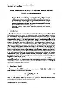
The main objective of the control is to regulate the biomass concentration X to a reference value X re f . Now, the efficiency of the proposed control strategy is validated in simulation. The performances of the above mentioned algorithms are compared in a worst uncertain parameters case. The parameters values of the system are chosen on the parameter subspace border (θreal = [ρm+ , Ks− , µ¯ + , KQ− , KsI− , KiI+ ]) [11], where the uncertain parameters subspace [θ − , θ + ] is given by [0.8θnom , 1.2θnom ]. The maximal admissible dilution rate Dmax equals 1.6d −1 . The optimization was run on Microsoft PC (Intel(R) Core(TM) i7 − 3770, 3.40 GHz, 8GB Ram). Two predictive control laws will be tested (Fig. 1): the RNMPC (4) and the proposed one (LRMPC). The controllers tuning parameters are the same for both strategies (Ts =20 min, N p = 5 and V = W = INp ). It can be noticed the anticipation behavior to a setpoint change (Fig. 1), due to the prediction of the setpoint
4051
27.5
X(µm3 .L−1 )
27 26.5 27.15 26
27.1 27.05
25.5
setpoint RNMPC (Ts = 20 min)
27
25
0.4
LRMPC (Ts = 20 min)
0.45
LRMPC (Ts = 5 min)
24.5 0
0.1
0.2
0.3
0.4
0.5
0.6
0.7
0.8
0.9
1
0.6
0.7
0.8
0.9
1
Time [d]
2
D (d−1 )
1.5
1
0.5
0 0
0.1
0.2
0.3
0.4
0.5
Time [d]
Fig. 1. Biomass concentration, tracking error and dilution rate evolution with time for LRMPC and RNMPC strategies.
trajectory future evolution over the moving horizon. On the other side, the obtained results show that RNMPC has better performances than the LRMPC controller under parameter uncertainties. In the case of LRMPC, the output is not able to track the specified setpoint in the presence of parameters uncertainties, due to the approximation of the model through linearization. When reducing sampling time (see Fig. 1 for results with Ts = 10 min), the static error is reduced. The steady state error could be further reduced by adding a PI controller [12]. In addition, the LRMPC offers a very significant computational load reduction comparing with the RNMPC as shown in the Table II. In fact, this can be explained by the fact that RNMPC is an optimization problem of dimension N p × Nθ while LRMPC is an unidimensional optimization problem with a quadratic programming problem. Consequently, when considering a more complex model with a greater number of state variables and parameters, the computation time increases in the RNMPC strategy. TABLE II C OMPARISON OF THE PROPOSED ALGORITHMS . Computation time (s)
``` Perf. indices ``` ``` min Algo. RNMPC LRMPC
0.764 0.577
mean
max
8.109 0.896
39.234 1.139
VI. C ONCLUSIONS AND FUTURE WORK In this paper we have presented a new robust MPC with guaranteed robust stability. Considering a process model with parameters that are within a given confidence
intervals, the robust MPC is designed in order to take into account these parameters uncertainties. The minmax problem is solved in two ways: first, the optimal control sequence is determined so that the maximum deviation for all trajectories overall possible data scenarii is minimized. Secondly, a linearization of the predicted trajectory is performed to turn the original optimization problem into a more tractable one. Moreover, the stability is analysed. Several simulations were performed in order to compare the LRMPC strategy to the classical RNMPC in the case of model parameters uncertainties. The LRMPC ensures a good trade-off between computational load and tracking trajectory accuracy. Future research will focus on the impact of the convergence and feasability of the optimization algorithm on the stability and performance of the control law. In future work, an interesting perspective in order to increase the quality of the linearized model used for prediction, may be considering a second order expansion rather than the first order approximation of the nonlinear model. Handling instructured uncertainties by the controller should be also investigated. R EFERENCES [1] E. F. Camacho and C. Bordons, Model Predictive Control. Springer London, 2004. [2] E. C. Kerrigan and J. Maciejowski, “Feedback min-max model predictive control using a single linear program: Robust stability and the explicit solution,” Int. J. Robust Nonlinear Control, vol. 14, pp. 395–413, 2004. [3] D. Limon, T. Alamo, and E. Camacho, “Robust stability of minmax MPC controllers for nonlinear systems with bounded uncertainties,” Proceeding of the mathematical Theory of Networks and Systems, 2004. [4] L. Magni and R. Scattolini, Robustness and robust design of MPC for nonlinear discrete-time systems. Springer-Verlag, 2007, vol. 358. [5] D. Raimondo, D. Limon, M. Lazar, L. Magni, and E. Camachp, “Min-max model predictive control of nonlinear systems: A unifying overview on stability,” European Journal of Control, vol. 5, pp. 5–21, 2009. [6] L. Biegler, X. Yang, and G. Fischer, “Advances in sensitivitybased nonlinear model predictive control and dynamic real time optimization,” J. of Process Control, vol. 30, pp. 104–116, 2015. [7] D. Dochain, Automatic control of bioprocesses, D. Dochain, Ed. Editor. John Wiley & Sons, 2008. [8] A. H. Sayed, V. H. Nascimento, and F. A. M. Cipparrone, “A regularized robust design criterion for uncertain data,” SIAM J. MAT. ANAL. APPL., vol. 32:4, pp. 1120–1142, 2002. [9] P. Masci, F. Grognard, and O. Bernard, “Microalgal biomass surface productivity optimization based on a photobioreactor model,” Proc. of the 11th CAB Conf., pp. 180–185, 2010. [10] G. Goffaux and A. Vande Wouwer, “Design of a robust nonlinear receding-horizon observer-Application to a biological system,” Proc. of the 17th IFAC World Congress, pp. 15 553–15 558, 2008. [11] S. E. Benattia, S. Tebbani, D. Dumur, and D. Selisteanu, “Robust nonlinear model predictive controller based on sensitivity analysis - application to a continuous photobioreactor,” Proc. of the 2014 IEEE MSC, pp. 1705–1710, 2014. [12] S. E. Benattia, S. Tebbani, and D. Dumur, “Hierarchical predictive control strategy of microalgae culture in a photobioreactor,” Proc. of the 19th International Conference on System Theory, Control and Computing, pp. 231–236, 2015.
4052