A Meshless Approach in Solution of Multiscale Solidification Modeling

Materials Science Forum 649 (2010) pp 211-216 © (2010) Trans Tech Publications, Switzerland doi:10.4028/www.scientific.net/MSF.649.211

A Meshless Approach in Solution of Multiscale Solidification Modeling Božidar Šarler1,a, Gregor Kosec1,b, Agnieszka Lorbicka1,c and Robert Vertnik2,d 1

Laboratory for Multiphase Processes, University of Nova Gorica, Vipavska 13, SI-5000, Nova Gorica, Slovenia 2

Research and Development, Štore-Steel, SI-3220 Štore, Slovenia

a

[email protected], [email protected], [email protected], d [email protected]

Keywords: Solidification, multiscale modeling, phase field method, meshless methods.

Abstract. This paper describes an overview of a new meshless solution procedure for calculation of one-domain coupled macroscopic heat, mass, momentum and species transfer problems as well as phase-field concepts of grain evolution. The solution procedure is defined on the macro [1] as well as on the micro levels [2] by a set of nodes which can be non-uniformly distributed. The domain and boundary of interest are divided into overlapping influence areas. On each of them, the fields are represented by the multiquadrics radial basis functions (RBF) collocation on a related sub-set of nodes. The time-stepping is performed in an explicit way. All governing equations are solved in their strong form, i.e. no integrations are performed. The polygonisation is not present and the formulation of the method is practically independent of the problem dimension. The solution can be easily and efficiently adapted in node redistribution and/or refinement sense, which is of utmost importance when coping with fields exhibiting sharp gradients. The concept and the results of the multiscale solidification modeling with the new approach are compared with the classical meshbased [3] approach. The method turns out to be extremely simple to code and accurate, inclusion of the complicated physics can easily be looked over. The coding in 2D or 3D is almost identical. Introduction The modeling of solid-liquid phase changes first evolved through posing of the governing equations for pure substances without any solution [4], subsequent analytical solution of the governing equations [5], and finally, solution by numerical methods [6]. The initially focused pure substances have been gradually replaced by the multicomponent materials, described by the multiphysics and multiscale models. The classical continuum mechanics description was upgraded and complemented by some sort of averaging and additional concepts like the phase field or cellular automata methods [7] have been introduced. The most popular discrete approximate methods for solving related models are nowadays the finite difference, finite volume, the finite element, and the boundary element methods. Despite the powerful features of these methods, there are often substantial difficulties in applying them to realistic, geometrically complex three-dimensional transient problems. A common drawback of the mentioned methods is the need to create a polygonization, either in the domain and/or on its boundary. This type of meshing is often the most time consuming part of the solution process and is far from being fully automated. This is even more pronounced in modeling of solidification systems, where in the front tracking approach, the polygons need to fit to the moving boundary, and in the one-domain approach, the polygons have to be refined in the vicinity of the moving boundary jumps and/or gradients. The selection of proper numerical method for solving related solidification models is still an open issue, quite easily demonstrated through discrepancy of the different numerical results of the classical benchmark tests [8,9]. This fact is probably due to the highly convective situations with All rights reserved. No part of contents of this paper may be reproduced or transmitted in any form or by any means without the written permission of the publisher: Trans Tech Publications Ltd, Switzerland, www.ttp.net. (ID: 193.2.120.205-04/02/10,14:54:47)

212

Solidification and Gravity V

sharp thermal and solutal gradients, characterized by the low Prandtl (0.01), high Schmidt numbers (100), and high thermal (10e7), and solutal (10e11) Rayleigh numbers. The meshless, sometimes also called mesh-free or mesh reduction methods, establish a solution of the problem domain and boundary without polygonisation [10]. Meshless methods use a set of nodes scattered within the problem domain and boundaries for representation of the domain geometry and fields. These sets of scattered nodes do not form a polygonisation (mesh), which means that no information on the geometrical connections between the nodes is required. There exist several types of meshless methods [10]. The discussion in this article is limited to the recent advances in meshless methods with the RBF’s [11]. They are characterized by the following features: the governing equations are solved in its strong form, collocation is used to represent the fields, the complicated physics and geometry can be easily coped with, the formulation is almost independent on the problem dimension, no polygonisation is needed, no integrations are needed, the method is very efficient, the method is very accurate, it has low numerical diffusion, and the method is simple to learn and to code. Basis of the Method Macroscopic Models and Microscopic Phase-fieled Models. Let us first describe the basis of the method, applicable in macroscopic multi-physics simulations as well as microscopic phase-field method. The suitable model equation for this purpose is the general transport equation, defined on a fixed domain Ω with boundary Γ ∂ (1) ( ρ Φ ) + ∇ ⋅ ( ρ vΦ ) = ∇ ⋅ ( D∇Φ ) + S , ∂t with ρ , Φ, t , v, D, and S standing for density, transport variable, time, velocity, diffusion matrix and source, respectively. The solution of the governing equation for the transport variable at the final time t0 + ∆t is sought, where t0 represents the initial time and ∆t the positive time increment. The

initial value of the transport variable Φ ( p,t ) at a point with position vector p and time t0 is defined through the known function Φ 0 . The boundary Γ is divided into not necessarily connected parts Γ = Γ D ∪ Γ ∪ Γ R with Dirichlet, Neumann and Robin type boundary conditions, respectively. At the boundary point p with normal nΓ and time t0 ≤ t ≤ t0 + ∆t , these boundary conditions are defined through known functions Φ ΓD , Φ Γ , Φ ΓR , ΦΓRref . The representation of function over a set l of (in general) non-equally spaced l nodes l p n ; n = 1,2,..., l is made in the following way lK

Φ ( p ) ≈ ∑ lψ k ( p ) l α k ,

(2)

k =1

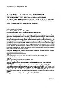
where lψ k stands for the shape functions, l α k for the coefficients of the shape functions, and l K represents the number of the shape functions. The left lower index on entries of expression (2) represents the sub-domain l ω on which the coefficients l α k are determined. The sub-domains l ω are overlapping (see Fig.1 right). Each of the sub-domains l ω includes l grid-points of which

Ω are in the domain and l Γ are on the boundary. The coefficients can be calculated from the sub-domain nodes in two distinct ways. The first way is collocation (interpolation) and the second way is approximation by the least squares method. Only the simpler collocation version for calculation of the coefficients is considered in this text. Let us assume the known function values l

l

l

K

Φ n in the nodes l pn of sub-domain l ω . The collocation implies ∑ lψ k ( l p n ) l α k = Φ ( l p n ) . For k =1

the coefficients to be computable, the number of the shape functions has to match the number of the

Materials Science Forum 649

collocation l

points,

and

the

collocation

matrix

213

has

to

be

non-singular

K

∑ψ ( l

k

l

p n ) l α k = Φ ( l p n ) ; l K = l . This system of equations can be written in matrix-vector form

k =1

Figure 1: Schematics of domain and boundary discretisation in mesh based methods (left) and meshless method (right), where the overlapping sub-domains replace the non-overlapping polygons.

and the coefficients l

l

α can be computed by inverting it

l

ψlα = lΦ ;

ψ

l

kn

= lψ k ( l p n ) ,

Φ n = Φ ( l pn ) , l α = l ψ −1 l Φ . By taking into account the expressions for the calculation of the

coefficients l α , the collocation representation of function Φ ( p ) and the first derivatives can be expressed as (in Cartesian system) lK

l

k =1

n =1

Φ ( p ) ≈ ∑ lψ k ( p ) ∑ l ψ kn-1 l Φ n ,.

lK l ∂ ∂ ψ k ( p ) ∑ l ψ kn-1 l Φ n ; ς = x, y , z Φ (p ) ≈ ∑ ∂pς k =1 ∂pς n =1

(3)

The required second derivatives are calculated principally the same as the first ones. The radial basis 1/ 2

functions, such as multi-quadrics ψ k ( p ) = ( p − pk ) ⋅ ( p − p k ) + c 2 

can be used for the shape

function, where c represents the shape parameter. What follows elaborates the semi-explicit solution of the general transport equation (1), subject to the initial and boundary conditions. The general transport equation can be transformed into following expression by taking into account the explicit discretization

Φ = ( ρ0 / ρ ) Φ0 − ( ∆t / ρ ) ∇⋅ ( ρ0 v0Φ0 ) + ( ∆t / ρ ) ∇⋅ ( D0∇Φ0 ) + ( ∆t / ρ ) S0 ,

(4)

from which the unknown function value Φ n in grid-point p n can be explicitly evaluated. The complete solution procedure follows the below defined steps 1-4. Step 1: First, the initial conditions are set in the domain and boundary nodes and the derivatives required in the convective and diffusive terms are calculated from the known nodal values. Step 2: The equation (4) is employed to calculate the new values of the variable Φ n at time t0 + ∆t in the domain nodes. Step 3: What follows in steps 3 and 4 defines variable Φ n at time t0 + ∆t in the Dirichlet, Neumann, and Robin boundary nodes. For this purpose, the coefficients l α have to be determined from the new values in the domain and from the information on the boundary conditions in the step 3. Let us introduce domain, Dirichlet, Neumann, and Robin boundary indicators for this purpose. These indicators are defined as

ϒΩn

1; pn ∈ΓD 1; pn ∈Γ 1; pn ∈ΓR 1; pn ∈Ω D

R = , ϒΓn =  , ϒΓn =  , ϒΓn =  D

R 0; pn ∉Ω 0; pn ∉Γ 0; pn ∉Γ 0; pn ∉Γ

The coefficients l α are calculated from the system of equations

(5)

214

l

Solidification and Gravity V

∑

l

l

ϒ Ωn lψ k ( l p n ) l α k + ∑ l ϒ ΓDn lψ k ( l p n ) l α k

k =1 l

+∑ l ϒ Γ n k =1

k =1 l ∂ ∂ R p + ψ α ∑ l k (l n)l k l ϒ Γn lψ k ( l p n ) l α k = ∂nΓ ∂nΓ k =1

(6)

  l = l ϒ Ωn l Φ n + l ϒ ΓDn l Φ nD + l ϒ Γ n l Φ n + l ϒ ΓRn l Φ ΓRn  ∑ lψ k ( l p n ) l α k − l Φ ΓRref n   k =1  The calculation of the coefficients l α follows from the system of linear equations l Ψ l α = l b with the right hand side vector

l

b n = l ϒ Ωn Φ n + l ϒ ΓDnΦ nD + l ϒ Γ n Φ n − l ϒ ΓRn l Φ ΓRn l Φ ΓRref n

and system

matrix D

l Ψ nk = l ϒ Ωn lψ k ( l p n ) + l ϒ Γn lψ k ( l p n ) + l ϒ Γn

l  ∂ R  ∂ R + ϒ − Φ ψ p ψ p ( ) ( ) l k l n l Γn  l k l n l Γn ∑ lψ k ( l p n )  . ∂nΓ k =1  ∂nΓ 

Step 4: The unknown boundary values are set from Eq. (3). Additional Topics Adaptivity. The macroscopic one-domain and the phase-field approach for solving solidification problems on different scales require an adaptive refinement of the discretisation in the multiphase zones where high gradients of the fields occur. This can be accomplished through the following strategies in the present meshless method. The adaptivity with respect to the reduction of the typical node-distances (H-adaptivity) is in the meshless methods achieved by insertion or removal of the computational nodes (Fig.2 right). Only neighborhood of the nearby points needs to be redefined in such a process. Mesh-based methods require a complete repolygonisation of the new node vicinity. The adaptivity with respect to the redistribution of the nodes (R-adaptivity) is in the meshless methods achieved through solution of an additional equation, similar as in polygon based methods. However, only redefinition of the neighborhood of all points is needed in meshless methods in comparison with the repolygonisation of the whole domain in mesh based methods. The adaptivity with respect to the type of the collocation functions (P-adaptivity) is achieved by enhancing the number of the nodes in a sub-domain (Fig.3 center) or by adding additional functions to the collocation set (augmentation) at the constant number of nodes. These functions are usually constants and first order polynomials. Additional equations for these functions can be obtained by requesting the vanishing of the sum of their coefficients. In special cases, like singularities, high jumps of the phase field variable or in the convection dominated problems, the RBF’s are unable to properly represent the fields, unless very fine nodalisation is used. The augmentation functions might in such cases represent the type of singularity or suit the physics of the problem. Addition of arctan in phase field variable collocation or addition of the solution of the convection-diffusion problems in flow dominated cases are typical examples. This strategy is called X-adaptivity.

Figure 2: Schematics of the node adaptivity. Initial configuration with 36 nodes (left), R-adaptive configuration with the same number of the nodes (center) and H-adaptive configuration with 121 nodes (right).

Materials Science Forum 649

215

Figure 3: Schematics of the P-adaptivity. Initial configuration with five-nodded support (left), enhanced support (center) and upwind support (right) for velocity in the horizontal direction. Strategies for convection dominated situations. There exist many other strategies (in addition to augmentation and node refinement) for solving the convection dominated situations. Among them: the choice of the un-symmetric upstream neighborhood configuration (Fig.3 right), the calculation of the values of central sub-domain point in displaced upstream direction, and use of the simple characteristic procedure, which represents a combination of Lagrangean and Eulerian approaches. The pressure-velocity coupling can be calculated from the pressure Poisson and pressure correction Poisson equations which require solution of the sparse matrix for all pressure nodes at one time or solution of the related artificial Pressure diffusion equations. Recently, an efficient, entirely local pressure correction algorithm has been deduced [12]. Applications The new method has been first successfully applied to diffusion problems [13], convectiondiffusion problems [14], the classical De Vahl Davis problem [12], natural convection in porous media [15], and melting of the anisotropic metals [16]. Industrial applications on the macro-scale include solution of the thermal model of the direct chill casting of aluminum alloys [17] and continuous casting of steel [18] on moving (growing) computational domains. The method has been on the micro level applied for solving dissolution of primary particles in binary aluminum alloys by an R-adaptive solution procedure [19]. The behavior of the method for entirely non-uniform node arrangements has been elaborated in [20]. Current work is devoted to low Re number k-epsilon turbulence modeling and comparison of meshless solution with the classical finite volume and finite element solutions [8] of binary alloy solidification. Summary This article shows basic elements and reviews applicability of the entirely new generation of numerical methods for solving solid-liquid phase change models on multiple scales. The numerical tests, performed until now in the cited references, show much higher accuracy of the method as compared with the classical approaches. The method can cope with very large problems, since the computational effort grows approximately linear with the number of the nodes. The method appears efficient, because it does not require a solution of large systems of equations. Instead, small systems of linear equations have to be solved in each time-step for each node and associated sub-domain, probably representing the most natural and automatic domain decomposition. Respectively, the method is straightforwardly suitable for parallelization. Despite the fact, that the represented method behaves excellent, the underlying rigorous mathematical theory is still lacking - a situation, typical for the classical numerical methods several decades ago. Acknowledgement. This paper forms a part of the project J2-0099: Multiscale Modeling and Simulation of Liquid-Solid Systems, sponsored by the Slovenian Research Agency and 6th EU Framework project INSPIRE, MRTN-CT-2005-019296M.

216

Solidification and Gravity V

References [1] B. Šarler, in: Advances in Meshfree Techniques, edited by V.M.A. Leitao, C.J.S Alves, and C Armando Duarte, Springer, Germany (2007) p.257. [2] K.G.F. Janssens, in: Continuum Scale Simulation of Engineering Materials, edited by D. Raabe, F. Roters, F. Barlat, L.Q. Chen, Wiley-VCH, Germany (2004) p.297. [3] C.A. Gandin, J.L. Desbiolles, M. Rappaz, P. Thévoz: Metall.Mater.Trans., Vol. 30A (1999), p. 3153. [4] G. Lamé and E. Clapeyron, Ann. Chem. Phys., Vol.47, (1831), p.250. [5] B. Šarler, Eng.Anal. Vol. 16 (1995), p. 83. [6] J. Douglass and T.M. Gallie: Duke Math. J., Vol. 22 (1955), p. 557-571. [7] C.A. Gandin, M.Bellet: Modelling of Casting, Welding, and Advanced Solidification Processes –XI, (TMS, Warrendale 2006). [8] N. Ahmad, H. Combeau, J.L. Desboilles, T. Jalanti, G. Lesoult, J. Rappaz, M. Rappaz and C.Stomp: Metall.Mater.Trans., Vol. 29A (1998), p.617-630. [9] D. Gobin, D. Gobin and P. LeQuéré: Comp. Assist. Mech. Eng. Sc., Vol.198 (2000), p. 289. [10] G.R. Liu and Y.T. Gu: An Introduction to Meshfree Methods and Their Programming, (Springer Verlag, Berlin 2005). [11] M.D. Buhmann: Radial Basis Function: Theory and Implementations (Cambridge University Press, UK 2003). [12] G. Kosec and B. Šarler: Int. J. Numer. Methods Heat and Fluid Flow, Vol. 18 (2008), p. 868. [13] B. Šarler and R. Vertnik: Comput. Math. Applic., Vol. 51 (2006), p.1269. [14] R. Vertnik and B. Šarler: Int.J.Numer.Methods Heat and Fluid Flow, Vol. 16 (2006), p. 617. [15] G. Kosec and B. Šarler: CMES, Vol. 25 (2008), p. 197. [16] G. Kosec and B. Šarler: Cast Metals Research, in press. [17] R. Vertnik, M. Založnik and B. Šarler: Eng.Anal., Vol. 30 (2006), p. 847. [18] R. Vertnik and B. Šarler: Cast Metals Research, in press. [19] I. Kovačević and B.Šarler: Materials Science and Engineering, Vol. A413–A414 (2005) 423. [20] J. Perko and B.Šarler: CMES, Vol.19 (2007) p.55.