Citation: Cohen, S., G. Willgoose, and G. Hancock (2008), A methodology for calculating the spatial ...... N. Hovius, M. T. Brandon, and D. M. Fisher, pp. 55â74 ...
Click Here
JOURNAL OF GEOPHYSICAL RESEARCH, VOL. 113, F03027, doi:10.1029/2007JF000820, 2008
for
Full Article
A methodology for calculating the spatial distribution of the area-slope equation and the hypsometric integral within a catchment Sagy Cohen,1,2 Garry Willgoose,1 and Greg Hancock2 Received 23 April 2007; revised 5 May 2008; accepted 13 June 2008; published 23 September 2008.
[1] The area-slope relationship and the hypsometric curve are well known catchment descriptors. The main shortcoming of traditional area-slope and hypsometry extraction methods is their limited ability to represent heterogeneity within the catchment. Here we present a new methodology for explicit calculation of the spatial distribution, at a pixel scale within a catchment, of the area-slope parameters and the hypsometric integral. This method allows us to create a quantitative representation of the area-slope equation and the hypsometric integral which can potentially be used in a variety of geomorphologic applications. The results show that the spatial distribution of both the area-slope equation and the hypsometric integral are noisy at the pixel scale. In order to reduce the noise three averaging techniques were examined. Subcatchment-scale averaging was found to be the best at identifying the spatial distribution of the area-slope equation and hypsometric integral. At the subcatchment scale the spatial distribution of the area-slope equation and the hypsometric integral approximated the spatial distribution of soil morphological and geological units of the Goulburn River catchment in eastern Australia. The spatially distributed area-slope results were tested using manually extracted subcatchment average area-slope values and found to be well correlated. The spatially distributed hypsometric integral was also well correlated with landform concavity and convergence. The subcatchment-scale averaging of the spatially distributed area-slope equation and hypsometric integral is shown to be a promising tool for producing spatially distributed data. The techniques are demonstrated on a catchment that has marked spatial variation in soils and geology. The results show that the spatially explicit maps can potentially identify the spatial extent of these soil types and geological features and agrees well with existing soil maps. Citation: Cohen, S., G. Willgoose, and G. Hancock (2008), A methodology for calculating the spatial distribution of the area-slope equation and the hypsometric integral within a catchment, J. Geophys. Res., 113, F03027, doi:10.1029/2007JF000820.
1. Introduction [2] Soil functional properties vary systematically at the hillslope scale, and distributed process models (e.g., hydrology and erosion) would benefit from maps of soil functional properties for large catchments. For example, Bloschl et al. [1995] and Grayson et al. [1995] show that the spatial organization of saturated areas at the hillslope scale systematically impacts on the catchment-scale hydrograph. Accordingly there is significant interest in automated methods that can predict the spatial distribution of soil properties at the hillslope scale from easily measured geomorphic properties [McBratney et al., 2003]. Significant progress has been made in the past decade in describing the spatial distribution of area-slope and hypsometry for channels and linking this
1 School of Engineering, University of Newcastle, Callaghan, New South Wales, Australia. 2 School of Environmental and Life Sciences, University of Newcastle, Callaghan, New South Wales, Australia.
Copyright 2008 by the American Geophysical Union. 0148-0227/08/2007JF000820$09.00
distribution to dominant channel process [e.g., Tucker and Whipple, 2002]. Less progress has been made for describing hillslopes and linking these descriptions to the soil of the hillslopes [e.g., Minasny and McBratney, 2001, 2006]. Mapping the spatial distribution of area-slope and hypsometry within a catchment will allow us to explore explicit spatial links between geomorphology and erosion processes, morphology, surface concavity, soil characteristics, geology, etc. This would have direct applicability to digital soil mapping and soil pedogenesis modeling [Minasny and McBratney, 2006]. Maps of intracatchment soil spatial distribution would also improve models for hydrology and geomorphology that use the area-slope relationship [e.g., Willgoose and Perera, 2001]. [3] In this paper we describe and explore new automated algorithms for calculating the area-slope equation and hypsometric integral at a pixel scale thus providing highresolution maps of the intracatchment variability of these properties. We also provide a preliminary demonstration of these techniques by predicting the spatial distribution of soils in a test catchment where soils maps are available for comparison.
F03027
1 of 13
F03027
COHEN ET AL.: SPATIALLY DISTRIBUTED AREA-SLOPE
F03027
the temporal average erosion rate (r Qs) or (2) assuming spatially uniform erosion equal to U leading to @z ¼ U þ rQs ¼ 0; @t
ð2Þ
where z is the elevation, t is time and Qs is the sediment flux. An integral solution at any point of the catchment with a known area draining through it (A) leads to � UA ¼ Qs ¼ fQs ðQ; S Þ ¼ fQs fQ ð AÞ; S ;
ð3Þ
where Q is the runoff discharge through a point. This allows us to solve the area-slope relationship for different erosion processes. Using simple sediment flux and discharge equation (Qs = b 1 Qm1Sn1 and Q = b 3 Am3 respectively) for transport-limited fluvial process in equation (3) leads to the area-slope relationship [Willgoose et al., 1991] � S¼
Figure 1. A typical transport-limited area-slope relationship log-log curve. The dashed line indicates the transition point between the diffusive-dominated regions on the left and fluvial-dominated regions on the right. [4] Researchers have observed and measured the relationship between contributing area and local slope in channels [e.g., Horton, 1945; Hack, 1957; Flint, 1974; Sklar and Dietrich, 1998] and hillslopes [Gilbert, 1909]. Flint [1974] described a general power law relationship between the slope and stream magnitude that is approximately equivalent to S ¼ cAa ;
ð1Þ
where S is the local slope, A is the contributing area, c is a slope-scaling constant and a is the exponent coefficient. In a catchment dominated by transport-limited erosion processes a typical log-log area-slope curve exhibits two distinct regions (Figure 1), a diffusive dominated region on the left-hand side (low area values) and a fluvial dominated region on the right-hand side (high area values [Willgoose et al., 1991; Willgoose, 1994; Hancock and Willgoose, 2002; Hancock, 2005; Grimaldi et al., 2005; Hancock and Evans, 2006]). The diffusive region has been interpreted to be dominated by processes such as rainsplash, soil creep and interrill erosion accruing on hillslopes while the fluvial region is associated with channel erosion processes [Tarboton et al., 1992; Hancock, 2005; Hancock and Evans, 2006]. The two regions are also associated with landform concavity with the diffusive dominated region generating concave down landforms and concave up landforms generated in the fluvial dominated region. Willgoose et al. [1991] and Willgoose [2001] provided mathematical expressions for the two regions in the catchment. Their numerical solution was based on either (1) assuming dynamic equilibrium in which the tectonic uplift (U) is balanced by
U 1 b1 bm 3
�n1
1
A
1�m1 m3 n1
/ Aa ;
ð4Þ
where b 1, m1, n1, b 3 and m3 are parameters that are generally considered, for the purposes of area-slope analyses, constant in space and time and where a is referred to as the area exponent. [5] On the basis of Qs = DS [Gilbert, 1909] the areaslope relationship for the diffusive erosion process is [Willgoose et al., 1991] S¼
� � U a A ; D s
ð5Þ
where D is hillslope diffusivity or creep, a = 1, and As is the specific area (area draining to that point per unit width). The difference between fluvial and diffusive erosion processes that arise from equations 4 and 5 are the constant and exponent of equation 1 (c and a respectively). A similar argument can be followed for detachment limited erosion processes, with the c being a function of uplift and detachment rate, and the a a function of the discharge and slope dependence on detachment [Moglen and Bras, 1995]. We can therefore assert that the spatial distribution of c and a within a heterogeneous catchment is significant and a function of erosion process. [6] The other geomorphic descriptor we will examine in this paper is the hypsometric curve (Figure 2 [Strahler, 1964; Willgoose and Hancock, 1998]). The hypsometric curve is a nondimensional area-elevation relationship which allows ready comparison of catchments and is traditionally associated with different stages of catchment maturity [Strahler, 1964]. Willgoose and Hancock [1998] demonstrated a link between the hypsometric curve and different erosion processes, catchment geometry and network form. The hypsometric integral is the area under the hypsometric curve and provides a quantitative value for comparing catchments. Walcott and Summerfield [2007] found a strong spatial trend in the distribution of the hypsometric integral and a correlation to the erosion resistance of lithologies. Using Willgoose and Hancock’s [1998] classification, a higher hypsometric integral values (greater then 0.5) represent catchments dominated by diffusive erosion processes
2 of 13
F03027
COHEN ET AL.: SPATIALLY DISTRIBUTED AREA-SLOPE
F03027
The approach is applied to a large catchment with heterogeneous soils. The resulting, automatically calculated, areaslope parameters are tested against manually extracted areaslope parameters for selected subcatchments on different soils. The hypsometric integral is compared to two independent descriptors of landscape curvature. We will show that the results reveal correlations between the geomorphic parameters and the spatial distribution of soils, morphology and geological features.
2. Study Site
Figure 2. Two typical hypsometric curves. The dashed curve represents a concave down landform associated with diffusive dominated catchments, while the solid line represents a concave up landform associated with fluvial dominated catchments. (concave down hypsometric curve; Figure 2) while lower values (less then 0.5) represent fluvial dominated catchments (concave up hypsometric curve). We therefore assert that the hypsometric integral is linked to erosion process, and landform curvature and its landscape morphology. [7] Conventional calculation of the area-slope equation and hypsometric integral requires plotting the relevant variables for a complete catchment and manually extracting either the power law equation of the area-slope curve or the integral of the hypsometric curve. In recent years a more spatially distributed approach has been adopted in channel research. For example, Seidl and Dietrich [1992] and Sklar and Dietrich [1998] have solved the area-slope equation for principle and tributary channels, Wobus et al. [2006] have solved it at channel junctions, while Brocklehurst and Whipple [2004] calculated the hypsometric integral in many catchments exploring its variation for different environments. Walcott and Summerfield [2007] introduced a new method for calculation of subcatchment hypsometric integral. These recent works while an advance in whole catchment analysis remain spatially limited since most are manually calculated for each catchment (or subcatchment) limiting the number of units investigated and thus the spatial resolution that is practical. By comparison, the spatial distribution of hillslope geomorphic properties and any relationship to soils and/or geology have only been lightly researched [e.g., Dietrich et al., 1993; Willgoose, 2001]. Recent advances in GIS based surface analysis tools allow us to develop automated algorithms to solve the area-slope equation and hypsometric integral at a pixel scale within a catchment. [8] This paper presents a new approach for automatically calculating the spatial distribution of the area-slope parameters and the hypsometric integral at a pixel scale within a catchment thus describing the intracatchment variability.
[9] The Goulburn River catchment (approx. 7000 km2) is located on the Upper Hunter Valley in New South Wales, Australia (Figure 3). The catchment can be divided into the following two distinct geological units: [10] 1. The northern Basaltic lava region which is a part of the Liverpool Range volcanic province. This region consist of mostly fertile soils [Galloway, 1963a] and rolling hills topography (except for the rocky slopes of the Liverpool Range to the extreme north of the catchment) [Galloway, 1963b]. [11] 2. The southern Sandstone region dominated by Triassic Sandstones exposed after erosion of the once overlaying basalt layer with a few basalt patches still visible on the cliff tops. Because of its high resistance to erosion the Sandstone region comprises rugged canyon terrain with shallow infertile soils [Galloway, 1963a] and wide floodplains along the main channels. [12] The climate is temperate with average yearly precipitation ranging from 1000 mm in the north to less than 500 mm at the center of the catchment [Australian Bureau of Meteorology, 1975]. Temperatures vary between an average minimum of 3°C in the coldest month (July) to an average maximum of 30°C in the hottest (January) [Australian Bureau of Meteorology, 1975]. [13] A 25 m square gridded digital elevation model (DEM) of the catchment derived from digitised 10 m contours (from Land and Property Information New South Wales (LPI)) was used for calculating the topographic descriptors in this work. C. Martinez et al. (An assessment of digital elevation models and their ability to capture geomorphic and hydrologic properties at the catchment scale, submitted to International Journal of Remote Sensing, 2008) examined the influence of DEM resolution on both area-slope plots and hypsometry of a subcatchment of the Goulburn River catchment located in the center of the study area. Using a range of high-resolution and accurate DEMs (ranging from 5 m resolution created by differential Global Positioning System to the LPI 25 m DEM used in this paper) they found little difference in manually extracted area-slope a and almost no difference in hypsometry. For the entire catchment domain of nearly 11 million cells there were less then 30 000 requiring pit filling, 0.27% of the cells. We are therefore confident in using our 25 m DEM to describe the topography of our study site for our work. [14] The National Australian soil map (1 km resolution; Figure 3) was used to distinguish between the five dominant soil types in the catchment. The northern basaltic region contains three main soil units: clay-loam on the northern ridges, clay on the central hills and loam in the southern parts. The southern sandstone region contains mostly sandy
3 of 13
COHEN ET AL.: SPATIALLY DISTRIBUTED AREA-SLOPE
F03027
F03027
Figure 3. The Goulburn catchment location, relief, and main soil groups. The viewshed presentation of the catchment DEM shows the clear distinction between the rolling hills topography in the northern clay, loam, and clay-loam soils to the rugged terrain in the southern sandy soils and the floodplains dominated by sandy loam soils.
soil with extensive sand-loam strips along the floodplains and a large isolated clay-loam patch in the south. This boundary between the soils of the northern and southern regions is quite sharp, and is easily distinguished in the field and in aerial photos.
the area draining into a node. Rearranging equation (6) leads to log Si � ai log Ai ¼ log Siþ1 � ai log Aiþ1 ;
ð7Þ
which is then used to extract ai
3. Spatially Explicit Calculation 3.1. Area-Slope [15] We based our numeric solution of the area-slope equation on Seidl and Dietrich’s [1992] approach. In its simplest form, the spatially explicit solution of equation (1) is based on assuming equal c in two adjacent nodes down the flow path ci ¼ ciþ1
Si Siþ1 ¼ ai ¼ ai ; Ai Aiþ1
� � log SSiþ1i � �: ai ¼ log AAiþ1i
Parameter ci is then calculated from equation (6) ci ¼
ð6Þ
where Si is the local topographic slope, Ai is the local contributing area, i is the node been calculated and i + 1 is the node immediately downstream. The contributing area is
ð8Þ
Si : Aai i
ð9Þ
[16] In this form the spatially explicit algorithm for solving equation (8) and (9) requires the following three input rasters: (1) contributing area (the number of inflowing pixels), (2) local slope, and (3) flow direction (the direction
4 of 13
COHEN ET AL.: SPATIALLY DISTRIBUTED AREA-SLOPE
F03027
to the steepest slope neighboring pixel). The flow direction raster is used to determine Ai+1 and Si+1 in equation (8). In this paper we used the Dinf algorithm [Tarboton, 1997] to calculate the contributing area map and then the D8 algorithm [O’Callaghan and Mark, 1984] to calculate the flow direction raster (used solely to determine the downstream node) since its relative simplicity allows an easier integration into the spatially explicit algorithm programmed in Fortran. [17] A more algorithmically complicated approach for spatially solving the area-slope equation uses several nodes along the flow path instead of the simple two node approach above. This requires least square regression to average several up and down flow nodes. Each node is then allocated the average area and slope values of its up and down flow node, potentially reducing DEM noise and errors. This method can be applied using as many up and down flow nodes as desired. The main downside of this approach is that it complicates the numerical solution since it requires the inheritance of values from several up and down flow cells instead of the simple use of a flow direction raster in the two node approach. The above calculations were done using a Fortran code with the D8 flow direction raster determined as described above. 3.2. Hypsometric Integral [18] As previously mentioned, the hypsometric integral is the area under the hypsometric curve (Figure 2). Calculating the hypsometric integral for a single catchment can be simplified by noting that the area under the curve is equal to the area of a rectangle which lies between 0 to 1 on the x axis (relative area) and 0 to mean relative elevation (y axis). Therefore the only variable is the mean relative elevation of a catchment. Our spatial distributed solution for the hypsometric integral then uses the normalization [Brocklehurst and Whipple, 2004]
HI ¼
Z � Zo ; Zmax � Zo
ð10Þ
where HI is the hypsometric integral, Zmax is the maximum elevation of the catchment, Z is the average elevation and Zo is the minimum or outlet elevation. [19] The algorithm for spatially explicit calculation of the hypsometric integral solves equation (10) for each pixel in the catchment using a Fortran code. Each pixel is considered a local catchment outlet and the parameters of equation (10) are the elevation characteristics of this local catchment. This algorithm requires the following three input rasters: (1) DEM for extracting the local outlet elevation (Zo), (2) average elevation (Z), and (3) maximum elevation (Zmax) of the catchment flowing into each pixel. These later two parameters were extracted by a Fortran code.
4. Results 4.1. Area-Slope Parameters [20] The distinct soil units in Goulburn catchment allow us to more clearly study the correlation between geological and geomorphologic characteristics, and the spatial distribution of a and c. If our hypothesis that geomorphic parameters are related to soil type is correct then the distinct
F03027
Figure 4. The area-slope relationship for each soil unit in the Goulburn River catchment. Each point is the average slope for all pixels with the same area. boundaries between the soil types implies that our spatially distributed analyses should also yield distinct regions. The area-slope plot in Figure 4 was created by averaging the slope values of all the pixels with similar area value. For example, the point for area = 1 (i.e., one pixel) is the average slope of all the pixels in the catchment with this area value. This technique enables us to avoid plotting the whole pixel-scale database (over 10 � 106 pixels). It also reduces noise and scatter in the plots so that we can better observe mean trends. This technique is used for all the spatial distributed plots in this paper. Figure 4 shows distinct differences in the area-slope parameters between the different soil units. The clay, clay-loam and loam curves (typically found on the northern part of the catchment) have generally higher a values compared to the sand and sandloam curves and their y intercept values (c) are generally higher. Figure 4 demonstrates that distinguishing between the different soil units and even between the two major geological groups is not possible in all parts of the plot using either a or c separately, nor that for that matter slope on its own. This suggests that both a and c are needed and that together they provide more spatial information than contributing area or slope values alone. 4.1.1. Spatial Distributed a [21] The spatially distributed a raster exhibits considerable noise with unreasonably high and low extreme values. Those extreme values are the result of small differences in slope, or jumps in the contributing area between two adjacent pixels. Although it may be a natural feature, and despite the fact that they account for a small proportion of pixels (approx. 2%), they severely mask the majority of reasonable values because of their high value (up to a factor of 3). In order to deal with those extreme values we constrained the a values between assigned minimum and maximum thresholds. We examined the following two
5 of 13
F03027
COHEN ET AL.: SPATIALLY DISTRIBUTED AREA-SLOPE
Figure 5. Area-slope relationship of the two constrained a methods. Each point is the average slope for all pixels with the same area. Method 1 (crosses) excluded all outliers larger than 2 and smaller than �2. Method 2 (squares) limited the outliers to fit between 2 and �2 (higher or lower values were assigned with the maximum and minimum value, respectively). constraint approaches: (1) excluding the extreme values by assigning a ‘‘no data’’ value and (2) including them by assigning a maximum or minimum threshold value. The sensitivity of the threshold value was explored by executing the spatially explicit a algorithm with a range of thresholds, finding the one that resulted in the best fit to the a values that we extracted from the area-slope plot (Figure 4). The threshold values we found to be the best fits were ±2. [22] We used the threshold value in the two constraining methods and compared the three resulting area-a plots (unconstrained and two constrained methods). Significant differences were found. The unconstrained area-a plot shows considerable scatter and no distinct differences between the five soil types while the two constrained a rasters exhibited a much cleaner plot. The area-a curve of constraint method 2 shows lower values than method 1 (Figure 5) and better represents the manually extracted a values from the areaslope plot. We therefore used method 2 for the remaining analysis. [23] The area-a plot for constraint method 2 (Figure 6) clearly distinguishes between the two major geological units but still shows considerable scatter for higher area. The a spatial distribution raster (Figure 7a) shows that while constraining the extreme a values reduces the noise so that the spatial pattern is clearer, a visual identification of morphological, geological or soil units remains difficult. [24] In order to reduce the noise three smoothing techniques were explored. In the first technique, least square regression was used in the spatially explicit algorithm (section 3.1). We examined the use of least square averaging over 3 (one up and one down flow) and 5 pixels (two up and two down flow). The result did not significantly reduce the noise.
F03027
[25] In the second technique a low-pass filter was applied. A low-pass filter removes noise by averaging the values of a fixed sized pixel window. We used a 3 � 3 pixel window. The resulting raster was smoother and improved our ability to identify spatial patterns but still contained considerable noise. [26] In the third technique a was averaged at a subcatchment scale. The subcatchment layer was calculated from a 25 m DEM using the TauDEM (D. G. Tarboton, Terrain Analysis Using Digital Elevation Models (TauDEM), Utah State University Logan, 2006, available at: http://hydrology. neng.usu.edu/taudem) tools package embedded into ArcGIS. We used Strahler channel order as a threshold variable controlling the scale of the subcatchments. Selecting a lower channel order results in smaller subcatchments and therefore more subcatchments per catchment. We examined a range of channel orders and found that the fourth order resulted in a layer with too much detail (over 40 000 subcatchments), while the eight order resulted in too few with less then 90. We therefore averaged a in three subcatchment layers fifth, sixth, and seventh channel order (containing 9067, 1883, and 381 subcatchments, respectively; Figures 7b –7d). This selection is subjective and we expect the appropriate scale to vary between different catchments and applications. For example, Walcott and Summerfield [2007] found order 2 – 6 subcatchments to be the most appropriate for their hypsometric integral study. [27] Our subcatchment averaging merges the channel and hillslope pixels despite the potentially different statistics for each regime. We are confident doing so since channelized pixels account for only 1 –3% of the catchment area so that the effect of channel-hillslope mergence is statistically negligible. We tested this approximation by removing
Figure 6. Area-a relationship for each soil unit using constrained a method 2. Each point is the average a for all pixels with the same area. A clear difference can be observed between the northern soil units (clay, clay-loam, and loam) and the southern units (sand and sand-loam) for the lower area values.
6 of 13
F03027
COHEN ET AL.: SPATIALLY DISTRIBUTED AREA-SLOPE
Figure 7. Spatially distributed parameter a for (a) pixel scale and (b) fifth, (c) sixth, and (d) seventh channel order subcatchment scale. For the subcatchment-scale maps (Figures 7b– 7d) the value of each subcatchment is the average of the pixels within its boundaries. 7 of 13
F03027
F03027
COHEN ET AL.: SPATIALLY DISTRIBUTED AREA-SLOPE
Figure 8. Subcatchment-averaged a using all pixels versus subcatchment-averaged a excluding channelized pixels form two channels maps (calculated by using 100 and 50 pixels thresholds). channelized pixels from the a map and comparing it to the original map where channels are included. We repeated this exercise for two channel network maps with different contributing area threshold (50 and 100 pixels). These new a maps were averaged in the same way as the original map and compared to the original results. There is a nearly perfect linear correlation (R2 > 0.98; slope = 1.03; interaction