A model-based embedded control hardware/software co-design approach for optimized sensor selection of industrial systems Kyriakos M. Deliparaschos1 , Konstantinos Michail2 , Spyros G. Tzafestas3 , Argyrios C. Zolotas4 Abstract— In this work, a Field Programmable Gate Array (FPGA)-based embedded software platform coupled with a software-based plant, forming a Hardware-In-the-Loop (HIL), is used to validate a systematic sensor selection framework. The systematic sensor selection framework combines multi-objective optimization, Linear-Quadratic-Gaussian (LQG) control, and the nonlinear model of a maglev suspension. The physical process that represents the suspension plant is realized in a high-level system modeling environment, while the LQG controller is implemented on an FPGA. FPGAs allow to rapidly evaluate algorithms and test designs under real-world scenarios avoiding heavy time penalty associated with Hardware Description Language (HDL) simulators. Moreover, the HIL technique implemented shows a significant speed-up in the required execution time when compared to the software-based model. Index Terms— Sensor selection, embedded control, FPGA design, maglev, electromagnetic suspension, observer-based controller, Hardware-In-the-Loop, FPGA-In-the-Loop.
I. I NTRODUCTION A vast majority of control systems today are embedded in a sense that they rely on built in special purpose digital hardware to close their feedback loops. Embedded control systems are widely used in industrial control, transportation systems, robotics, automotive engineering, and many others. These type of systems interface with the external environment (i.e., sensors and actuators), are real-time critical (i.e., embedded control algorithm must execute in synchrony with the physical system under control, to guarantee performance and safety), and allow for distributed control (i.e., network of embedded controllers). A model-based embedded control software/hardware co-design approach is followed in this work. Modeling/simulation along with FPGA synthesis and HDL analysis tools (i.e., MATLAB/Simulink and Xilinx ISE) are used to enable rapid prototyping, autocode generation (i.e., generate HDL code from a Simulink model), HardwareIn-the-Loop (HIL) testing, and consider the functional correctness of the model-based design with the generated HDL in a co-simulation environment. The HIL technique is a method widely used in the development and testing of 1 K. M. Deliparaschos is with the Department of Electrical and Computer Engineering and Informatics, Cyprus University of Technology, Limassol, CY.
[email protected] 2 K. Michail is with Department of Electrical and Computer Engineering and Informatics, Cyprus University of Technology, Limassol, CY and SignalGeneriX Ltd, Limassol, CY.
[email protected] 3 S. G. Tzafestas is with the School of Electrical and Computer Engineering, National Technical University of Athens, GR.
[email protected]
4 A. C. Zolotas is with the School of Engineering, University of Lincoln, UK.
[email protected]
complex real-time control systems by effectively adding the complexity of the plant under control to the test platform [1], [2]. The model of the system is realized in a soft form and usually modeled using a high-level language (e.g., MATLAB) or a graphical model-based design tool (e.g., Simulink). An embedded control system is illustrated in Fig. 1, where the model of the plant (realized on software) interfaces with the actual controller (implemented on hardware) via a communication link. Physical process Software-based plant model
Fig. 1.
FPGA Communication protocol (Ethernet link)
Hardware-based controller
A simplified diagram of an embedded control system.
A typical high integrity system requires both control and reliable operation. Optimized performance, robustness, fault tolerance, and low complexity are the main goals of the designer. Industrial plants require a set of sensor nodes for acquiring measurements of the system. Part of this work is focused on minimizing the number of sensors selected from a large set such that the system is (i) stable, and (ii) satisfies a number of closed-loop performance criteria. The task of sensor set selection in an optimized manner for control design is a non-trivial task to do; especially if there is a large number of sensor candidates to select from. In [3], a framework for control and fault tolerance is proposed, which takes into account the aforementioned requirements for a non-trivial problem: the control of an electromagnetic suspension (EMS) for a maglev train [4]. The systematic framework combines LQG control [5], multiobjective optimization using genetic algorithms (GA) [6], and reconfigurable fault tolerant control methods [7]. The maglev EMS was used to test the efficacy of the framework and the results, implemented at a simulation level only, show good potential for industrial applications. In this paper, the validation of the framework is done via a model-based embedded control hardware/software co-design approach [8], [9], where a full LQG controller (combination of a Linear-Quadratic-Regulator (LQR) and a Kalman-Bucy Estimator (KBE)) is implemented on an FPGA chip and a HIL scheme is employed [10] for practical integration of the LQG controller on the FPGA chip [11] with the physical process describing the EMS plant under control, modeled in a high-level simulation environment (MATLAB/Simulink). In this setup, the control of an inherently unstable, nonlinear maglev EMS subject to a set of non-trivial control require-
ments (that industrial systems of such nature have), using the minimum number of sensors was studied. In [12], the authors presented some initial validation results of the systematic framework using the HIL technique targeted on FPGA, hereinafter referred to as FPGA-in-the-loop (FIL). While the KBE, as part of the LQG controller, was implemented on an FPGA chip, unlike our approach in this paper, the LQR was modeled in MATLAB/Simulink. The results show that the performance remains the same even if more sensors are added in the set. Moreover, the FPGA resource requirements are significantly reduced when fewer sensors are used to control the system. Finally, the FIL technique, as expected, shows a significant speed-up in the required execution time when compared to the software-based model. The rest of this paper is organised as follows. Section II outlines the modeling aspects of the maglev EMS system. Section III describes the systematic framework for optimized sensor selection with the FIL concept and Section IV introduces the LQG architecture and implementation on the FPGA. Analysis and simulation results from the practical LQG implementation with FIL as applied on the EMS are discussed in Section V. Section VI provides some final conclusions and discusses future directions. II. M ODEL AND CONTROL REQUIREMENTS OF THE EMS A. Non-linear model of the EMS The single-stage EMS that represents one quarter of a typical maglev vehicle, is based on a typical U-core shape electromagnet. Details on the particular modeling exercise, can be found in [4]. The non-linear model is described as follows, 8 N A K dZ t Vc IRc + c Gp2 b ( dz dI I > dt dt ) > = , B = Kb , < N A K c p b dt G + Lc (1) G 2 2 > dZ > : d Z = g Kf I , F = Kf B 2 , dG = dzt d2 t Ms G 2 dt dt dt
where Vc is the coil’s voltage, F is the vertical force, I is the coil’s current, G is the airgap, Z is the electromagnet’s position, and B is the flux density. The fixed parameters of the model are as follows: Ms is the vehicle’s mass, Rc is the coil’s resistance, Nc is the number of turns, Ap is the pole face area and zt is the track’s position. Kb , Kf and g reflect the flux, force and gravity constants (with values equal to 0.0015, 0.0221 and 9.81 m s 2 , respectively). The linearization of the non-linear model is based on small perturbations around the operating point, e.g., the airgap is assumed as G = Go + (zt z), where the lower case terms represent the small variation around the operating point, and subscript ’o’ refers to the operating point. A similar approach is followed for B, F , I, Vc and Z (b,f ,i,uc and z respectively). The linearized state-space description of the EMS, with state x , [i z˙ (zt z)]T and the full sensor set of the maglev y , [i, b, (zt z), z, ˙ z¨]T , is given by, ( x(t) ˙ = Ax(t) + Buc uc (t) + Bz˙t z˙t (t), (2) y(t) = Cx(t),
where, A is the 3 ⇥ 3 state matrix, Buc is the 3 ⇥ 1 input matrix, Bz˙t is the 3 ⇥ 1 disturbance matrix, and C is the ↵⇥3 output matrix (↵ varies from 1 to 5 (in this application), since its size changes according to the number of sensors in the sensor set). The various sensor sets can be obtained by appropriate selection of the corresponding rows in the output matrix C. Note that the linearized model of the EMS is used for the design of the LQG controller, whereas for the tuning of the controller as well as for the validation via FIL, the non-linear model is applied in the loop. B. Closed-loop control requirements The closed-loop design requirements for the EMS depend on the type and operating velocity of the train [13], and are affected by the magnitude of the input disturbances to the suspension. There are two types of disturbances that enter in the vertical direction of the EMS: (a) a stochastic behavior due to random variations of the rail position during vehicle movement; (b) a deterministic behavior [4] (considered in this work) occurs from the transition of the EMS onto the rail’s gradients. Assuming a total weight of 1000 kg, the operating point values for the EMS system become: Go = 0.015 m, Bo = 1 T, Io = 10 A, Vo = 100 V and Fo = 9810 N. Hence, the parameters of the electromagnets, based on the operating point of the EMS, were calculated as follows: Rc = 10 ⌦, Lc = 0.1 H, Nc = 2000 and Ap = 0.01 m2 . The deterministic disturbance here corresponds to a gradient of 5% at a vehicle speed of 15 m s 1 , an acceleration of 0.5 m s 2 , and a jerk of 1 m s 3 . The EMS must support the payload and follow the track gradients. As a result, there are specific boundaries where the EMS is allowed to operate: i) maximum airgap deviation, (zt z)p 7.5 mm; ii) maximum control effort, ucp 300 V; iii) settling time, ts 3 s, and iv) airgap steady state error, e(zt z)ss = 0. III. T HE SYSTEMATIC FRAMEWORK AND FIL
Any industrial plant has a number of control inputs {ui : i = 1, . . . nu }, input disturbances {di : i = 1, . . . nd } and a set of possible outputs, i.e., the full sensor set, Yf = {yi : i = 1, . . . ns }. Part of the problem is to determine the set of sensors, Yo ⇢ Yf , for which the system is (i) stable, (ii) satisfies a number of closed-loop performance criteria and (iii) has a minimum number of sensing elements in the selected set, i.e., the number of elements in Yo is minimal1 . The selection of Yo with respect to the aforementioned properties is a very important and complex process, especially if the plant has a large number of actuator/sensor configuration possibilities, i.e., sets. This work is focused upon optimized sensor selection, with respect to the aforementioned three properties. The full sensor set Yo is a subset of the full sensor set Yf . Many subsets of the full sensor set are possible to 1 This paper deals only with minimizing the number of sensors, however there are other objectives that could be meaningful for other than the EMS systems such as minimizing energy consumption, size of weight and cost.
Sensor measurements
be formed, and the number of them can be calculated from Ns = 2ns 1, where Ns is the total number of all sensor sets and ns is the total number of sensors. The LQG controller combines a Linear Quadratic Regulator (LQR) and a Kalman-Bucy Filter (KBE), hence its tuning is based on the separation principle as described in [5]; the framework algorithm is executed in two steps i.e., (i) In the first step, the LQR controller is optimized using a GA and the Pareto-optimality between the two objective functions, (i.e., 1 = irms and 2 = z¨rms ) is found. The LQR controller state feedback gains (i.e., Klqr = [Ki Kz˙ K(zt z) KR (zt z) ]), deduce the desired closedloop response which is then selected and accounted as the ‘ideal’ or reference response for the next step. (ii) The KBE is tuned for every feasible sensor set in order to achieve the ‘ideal’ closed-loop response. Finally, a table is provided with the optimized sensor sets, where the selection of the ’best’ sensor set is obtained based on the overall control constraint violation function, ⌦. This means that if there is one or more control constraint violations (see Section II-B for the EMS system) they are reflected in the evaluation of ⌦. If all control constraints are satisfied ⌦ = 0, otherwise its value depends on the level of the constraint(s) violation (i.e., the more pronounced the constraint violation is, the higher the value of ⌦). Figure 2 illustrates the FIL applied on the EMS where all five outputs, Yf , out of which only the Yo (i.e., the best sensor set) is fed into the FIL-based KBE.
+
+ + +
LQR
KBE
Software model (MAGLEV)
Fig. 2.
Estimated states
current gain K*u
velocity gain K*u
airgap gain K*u
fixpt scaling K*u
The discrete linear time-invariant KBE has the following state space form, C dx ˆ(k))
A(3,3)
A(2,3)
In3 A(1,3)
A(3,2)
Out3
Out2
A(2,2)
In2 A(1,2)
Out1
A(3,1)
Listing 1.
Optimized sensor selection framework validation using FIL.
d x ˆ˙ (k + 1) = Ad x ˆ(k) + Budc uc (k) + Klqg (y(k) yˆ(k) = C d x ˆ(k)
A(2,1)
A(1,1)
In1
(a)
Hardware model (LQG Controller)
IV. FPGA ARCHITECTURE OF THE LQG CONTROLLER
(
K*u
been calculated using the discrete time linear model of the EMS with a sampling rate of 10 kHz. Standard discretization procedure is followed here, hence full analysis is omitted. The design architecture of the LQG core implementation and its entity in Very High Speed Integrated Circuits (VHSIC) Hardware Description Language (VHDL) are depicted in Fig. 3a and Listing 1 respectively. The internal architecture of A3⇥3 block is illustrated in Fig. 3b, while a similar design 3⇥ approach is followed for C ↵⇥3 and Klqg blocks.
+ + +
K*u
Fig. 3. (a) LQG architecture for 3 sensor measurements (y1 , y2 , y3 ), (b) Internal architecture of A3⇥3 block.
Network fabric
+
Control input
(b)
Optimised sensor selection
Physical Process (Non-linear MAGLEV suspension model)
K*u
(3)
d where x ˆ are the estimated states, Klqg is the 3 ⇥ observer gain matrix ( is the number of sensors) that minimizes d E{[x x ˆ]T [x x ˆ]} (x represents the actual states). Klqg has
1 2 3 4 5 6 7 8 9 10 11 12 13 14 15 16 17 18 19 20
VHDL entity of the LQG core.
LIBRARY IEEE ; USE IEEE . s t d _ l o g i c _ 1 1 6 4 . ALL ; USE IEEE . numeric_std . ALL ; ENTITY LQG IS PORT( c l k rst clk_en control_in i_input_in b_in a_in ce_out uc_d_op i_op z_dot_op gap_op igap_op ); END LQG;
: : : : : : : : : : : : :
IN IN IN IN IN IN IN OUT OUT OUT OUT OUT OUT
std_logic ; std_logic ; std_logic ; s t d _ l o g i c _ v e c t o r (25 s t d _ l o g i c _ v e c t o r (31 s t d _ l o g i c _ v e c t o r (31 s t d _ l o g i c _ v e c t o r (31 std_logic ; s t d _ l o g i c _ v e c t o r (34 s t d _ l o g i c _ v e c t o r (35 s t d _ l o g i c _ v e c t o r (35 s t d _ l o g i c _ v e c t o r (34 s t d _ l o g i c _ v e c t o r (35
DOWNTO DOWNTO DOWNTO DOWNTO
0) ; 0) ; 0) ; 0) ;
sfix26_En19 sfix32_En28 sfix32_En35 sfix32_En31
DOWNTO DOWNTO DOWNTO DOWNTO DOWNTO
0) ; 0) ; 0) ; 0) ; 0)
sfix35_En27 sfix36_En24 sfix36_En23 sfix35_En23 sfix36_En23
The MATLAB HDL Coder tool was used in this work to automate and speed up the process of translating the high
level simulation model into an equivalent Register Transfer Level (RTL) HDL description. Due to MATLAB HDL Coder limitations in handling multi dimension matrices, a detailed LQG core model using explicitly scalar buses (see Fig. 3a and Listing 1) was developed prior to HDL translation. A. Quantization process An algorithm in a high level system modelling environment (such as MATLAB/Simulink) is represented in the floating-point domain, where mostly all variables are 64 bit allowing all operations to be performed in high precision format with large accuracy. In a digital implementation this translates to an increased number of flip-flops and combinational logic and inevitably results on a design that requires a large silicon area on the FPGA chip, large critical path that negatively affects speed, plus increased power consumption. To address the aforementioned problem, the algorithm under implementation (LQG in this work) has first undergone a conversion to the fixed-point domain and then modelled using VHDL. In the fixed-point domain, a pair of Wordlength, WL and Quality Fractional range, QF is considered for each parameter of the algorithm. As a consequence as (WL,QF) is increased will give a smaller Bit-Error Rate (BER) but larger silicon area, whereas as (WL,QF) is reduced will result to increased BER and smaller silicon area. Several simulations need to run to decide on the number of bits for (WL,QF) and the dynamic range of the parameters (MATLAB fixedpoint tool), in order to maintain a desired precision which will not compromise the overall system performance (i.e., destabilize the control loop), and maintain a low silicon area. The fixed-point range for a signed number ±a in a 2’s complement form is defined by the minimum and maximum value range a signed integer number type of Quantity Integer range (QI) bits can hold. The latter is best expressed by the inequality, 2QI 1 a 2QI 1 1 and can be rewritten, 2QI
1
a < 2QI
1
(4)
,a 2 Z
From (4) it can be easily shown that, QI|amin log2 ( a)+ 1 and QI|amax > log2 (a)+1. Since the positive constraint is the tighter one due to the asymmetry of signed integer types about zero, the constraint for the required number of bits can be generalised as, QI > log2 (max |[amin , amax ]|) + 1. Since QI is an integer number of bits we can truncate the result and add one to form an equation to compute QI (that satisfies the constraint QI > log2 (a)) such as, QI = b(log2 (max |[amin , amax ]|) + 2c. Assuming a resolution ✏ = 2 QF for the fractional part, the Quantity Fractional (QF) range becomes, QF = dlog2 (✏ 1 )e; hence, the required wordlength, WL (to sufficiently represent a float number to a fixed point representation) is given by the sum of QI and QF such that, W L|Req QI + QF or, 2QI
1
a < 2QI
1
2
QF
|✏=2
QF
(5)
B. FPGA design The FIL presented in this work was implemented on a Xilinx Virtex-6 ML605 development board. The ML605 board
utilizes a Xilinx Virtex-6 device (XC6VLX240T-1FFG1156) [14] in the 1156-pin fine-pitch Ball Grid Array (BGA) package, featuring 37, 680 slices2 and 768 special Digital Signal Processing (DSP) slices (DSP48A1). The LQG and the peripheral cores were synthesized using Xilinx Synthesis Tool (XST). A top-down manner [15] has been followed for the design process of the LQG controller (Fig. 4). The process initiates with the model specifications and requirements, advances to a high level functional system model (Simulink model) and continues on converting it to fixed-point prior to FPGA implementation. Co-simulation of the RTL model side-byside with the fixed-point Simulink model was performed using MATLAB’s HDL verifier and Mentor’s Modelsim simulator [16]. Moreover the implemented system on the FPGA chip was compared in real time using a cycle accurate Simulink model forming a FIL setup. Model specifications
Algorithmic analysis and implementation in floating point
Testbench
Diff
Model conversion in fixed point
Algorithm Stimuli
+
-
Results RTL design
Integration with peripheral cores (Ethernet MAC, DCM)
Implementation in RTL VHDL
Co-simulation with MATLAB HDL Simulator
Testbench
Diff
Logic synthesis
Algorithm Stimuli
FPGA device configuration
Fig. 4.
Place and Route
ML605 FPGA Board
+
-
Results
Ethernet link
FPGA-in-the-Loop simulation
FPGA hardware/software co-design and implementation flow.
V. R ESULTS ANALYSIS In this section, the results from the FIL used to validate the sensor selection framework are analyzed. As explained in Section III, the first step in the optimized sensor selection process is to choose the state vector Klqr . This is done based on three performance related criteria: (i) closed-loop vertical acceleration, z¨rms < 0.5 m s 2 , (ii) excitation coil’s current, irms < 2 A and (iii) best possible ride quality, i.e., min(¨ zrms ). The discretized LQR gains (Klqr ) are given as Ki = 245.67 V A 1 , Kz˙ = 3.349 ⇥ 103 V m 1 s, K(zt z) = 2.135 ⇥ 105 V m 1 and KR (zt z) = 24.03 V m 1 . The KBE in the second step of the framework is used to estimate the states, thus an optimized tuning of the KBE is necessary to accurately estimate the states from the LQR design (i.e., achieve the same performance with the LQR with various sensor sets). The optimization run has shown that 24 out of 31 sensor 2 Each
slice contains 4 Look Up Tables (LUTs) and 8 Flip-Flops (FFs).
TABLE I O PTIMIZED SENSOR SELECTION SIMULATION RESULTS . id 1 2 3 4 5 6 7 8 9
Sensor Set LQR response ! b (zt z) z¨ i, b i, z¨ i, b, (zt z) i, b, z¨ i, b, z, ˙ z¨ i, b, (zt z), z, ˙ z¨
Deterministic response X X 7 X X X X X X X
TABLE II D ESIGN UTILIZATION SUMMARY ( THREE SENSORS , iba ( ID :7), AND ONE SENSOR , b ( ID :1)).
⌦ X X 7 X X X X X X X
sets found to give the same closed-loop response as with the LQR one. Some of the corresponding results from the offline framework are presented in Table I. The first column is the sensor set identification number (id), the second column is the corresponding sensor set, and the next two columns show whether the deterministic response is satisfied (X) or not (7). The ⌦ function in the last column similarly indicates whether all control constraints described in Section II-B are fulfilled (X) or not (7). The selection of the best sensor set is done based on ⌦ as described in Section III. From a close inspection on the table, one can easily identify the best sensor set selection i.e., the one with the minimum number of sensor/s which satisfies all control requirements is id:1. In this work, the FIL was implemented for id:1 (single sensor), and is compared with id:7 (three sensors). The LQG implementation flow on the FPGA for other sensor set combinations follows the same approach.
Logic utilization Slice Registers Slice LUTs Occupied Slices Bonded IOBs Block RAMB36E1 Block RAMB18E1 BUFG DSP48E1s MMCM_ADVs
Used iba (id:7) b (id:1) 2410 2,354 4012 3777 1402 1362 30 30 2 2 1 1 5 4 73 69 1 1
Available 301,440 150,720 37,680 600 416 832 32 768 12
Utilization iba (id:7) b (id:1) 1% 1% 2% 2% 3% 3% 5% 5% 1% 1% 1% 1% 15% 12% 9% 8% 8% 8%
speeds were obtained with the map and place and route effort set to medium on Xilinx ISE 13.3. TABLE III D ESIGN UTILIZATION SUMMARY FOR THE LQG MODULE WITH iba ( ID :7) AND b ( ID :1) Module(iba) LQG KBE Ad Cd d Klqg LQR Module(b) LQG KBE Ad Cd d Klqg LQR
Slices 0/265 49/221 67/67 30/30 75/75 44/44 Slices 0/205 41/161 69/69 12/12 39/39 44/44
Slice Reg. 0/113 77/77 0/0 0/0 0/0 36/36 Slice Reg. 0/111 75/75 0/0 0/0 0/0 36/36
LUTs 0/884 170/717 221/221 99/99 227/227 167/167 LUTs 0/696 143/529 220/220 30/30 136/136 167/167
DSP48E1 0/73 1/50 27/27 14/14 8/8 23/23 DSP48E1 0/69 1/46 27/27 6/6 12/12 23/23
A. FPGA implementation for 2 sensor sets The resources requirements and trial and error quantization procedure are commented in this section. Table II show the logic utilization for the implemented integrated system on the FPGA device, for three and one sensor. The implemented design mainly includes the LQG core, ethernet Medium Access Control (MAC) [17] and the clock manager modules. The ethernet MAC core is licensed as part of the Xilinx Embedded Development Kit (EDK). According to the device utilization report from the Xilinx map (MAP) tool (see Table III), the LQG core module itself for id:7, occupies 265 slices, 113 slice registers, 884 slice LUTs, and 73 DSP cores (DSP48A1) and similarly for id:1, 205 slices, 111 slice registers, 696 slice LUTs, and 69 DSP48A1. A comparison of the utilized FPGA resources between three sensors, iba (id:7) and one sensor, b (id:1) LQG implementation scenarios, is depicted in Fig. 5, where one can easily see that the overall occupied area for id:1 onto the FPGA chip is significantly smaller when compared to the id:7 one. The implemented design uses one Mixed Mode Clock Manager (MMCM) module [18] that produces the different clocks inside the FPGA chip. The placed and routed FPGA designs (LQG and peripheral cores) for three and one sensor implementations, achieve according to post-place and route timing report a system clock operating frequency of 34.364 ns or 29.1 MHz, and 32.819 ns or 30.5 MHz respectively. The aforementioned
B. Data analysis from FIL simulations Figure 6 depicts the performance of the EMS using two sensor sets. One with single sensor (id:1) and the the other one with three (id:7). Specifically, Fig. 6a compares the airgap deflection error from simulation-based continuoustime and FIL-based discrete-time KBE with id:1 (top) and id:7 (bottom). The performance of the EMS is within the performance objectives listed in Section II-B. The airgap error magnitude between the simulation and FIL is in the order of 10 4 m which is fairly small. The state estimation of the LQG using id:1 is shown in Fig. 6b. All three states (i, z˙ and zt z) are accurately estimated using one sensor (b), which is similar to the state estimation achieved if more sensors were added, i.e., id:7 concluding that the EMS performs adequately with fewer sensors. VI. C ONCLUSIONS A semi-practical modeling and validation of an embedded control system for sensor optimization on a EMS plant using the FIL concept was presented. The physical process for the EMS is modeled in a high-level MATLAB/Simulink environment and the LQG controller is implemented on an FPGA. A model-based design approach has been followed for the FIL implementation using a fusion of system modeling and hardware/software co-design. The effect of fixed-point
0
LQG KBE
0.03 0.02
0
0.01 0.01 0.00 0.00
LQG KBE
2.99 2.99
4 2
LQR
Fig. 5.
6 1.04 1.56
D of available
0.11 0.11
0.15 0.09
0.07 0.02
0.2
0.15 0.15
0.11 0.10
0.4
8 3.52 3.52
0.59
10
LQR
DSP48E1
12
0.47
0.6
LQG KBE
1.82 0.78
LUTs
0.00 0.00
0
LQR
0.8
0.04 0.04
0.01 0.00 0.00
0.12 0.12
0.21 0.12
LQG KBE
0.02
0.13 0.13
0
0.09 0.02
0.2
0.19 0.17
0.13 0.12
0.4
0.03
9.51 8.98
0.6
D of available
0.04
0.54
D of available
0.8
D of available
Slice Registers
0.74
Slices
LQR
FPGA resources comparison for id:7 and id:1.
4
x 10 6 4 2 0
0
1
2
3
4
5
6
1
2
3
4
5
6
4
x 10 6 4 2 0
0
(a) Current with LQR Estimated current with FIL
4 2 0
0
1
2
3
4
5
6
Velocity with LQR Estimated velocity with FIL
0.6 0.4 0.2 0
0
1
2
3
4
5
6
#3
x 10 6
Airgap with LQR Estimated airgap with FIL
4 2 0
0
1
2
3
4
5
6
(b) Fig. 6. (a) Airgap error with id : 1, id : 7, (b) State estimation with id : 1.
quantization was analyzed early in the design process and the wordlength was optimized to yield a smaller implementation. System level test benches were used with HDL co-simulation to verify the HDL implementation, and also FIL simulation to significantly accelerate the system validation. The FIL
obtained results for the LQG implementation for two sensor sets (id:1 and id:7) were compared. The results clearly show that the LQG implementation in FIL is successful in spite of the complex quantization procedure and that the FIL approach greatly reduces simulation time when compared to the software-based model counterpart. R EFERENCES [1] R. Isermann, J. Schaffnit, and S. Sinsel, “Hardware-in-the-loop simulation for the design and testing of engine-control systems,” Control Engineering Practice, vol. 7, no. 5, pp. 643–653, 1999. [2] B. Lu, X. Wu, H. Figueroa, and A. Monti, “A low-cost real-time hardware-in-the-loop testing approach of power electronics controls,” IEEE Transactions on Industrial Electronics, vol. 54, no. 2, pp. 919– 931, 2007. [3] K. Michail, A. Zolotas, and R. M. Goodall, “Optimised configuration of sensors for fault tolerant control of an electromagnetic suspension system,” International Journal of Systems Science, vol. 43, no. 10, pp. 1785–1804, 2012. [4] K. Michail, “Optimised configuration of sensing elements for control and fault tolerance applied to an electro-magnetic suspension system,” 2009. PhD dissertation, Loughborough University, Department of Electronic and Electrical Engineering. http://hdl.handle.net/2134/5806. [5] S. Skogestad and I. Postlethwaite, Multivariable Feedback Control Analysis and Design. New York: John Wiley & Sons Ltd, 2nd Edition, 2005. [6] A. Konak, D. W. Coit, and A. E. Smith, “Multi-objective optimization using genetic algorithms: A tutorial,” Reliability Engineering and System Safety, vol. 91, no. 9, pp. 992–1007, 2006. [7] Y. Zhang and J. Jiang, “Bibliographical review on reconfigurable faulttolerant control systems,” Annual Reviews in Control, vol. 32, pp. 229– 252, 12 2008. [8] A. Forrai, Embedded Control System Design: A Model Based Approach. Springer Science & Business Media, July 2012. [9] R. Alur, D. Hristu-Varsakelis, K.-E. Arzen, W. Levine, J. Baillieul, and T. A. Henzinger, eds., Handbook of Networked and Embedded Control Systems. Boston: Birkhauser, 1st ed. 2005. corr. 2nd printing 2008 edition ed., June 2008. [10] M. Bacic, “On hardware-in-the-loop simulation,” in 44th IEEE Conference on Decision and Control and European Control Conference., pp. 3194–3198, 2005. [11] O. Lucia, O. Jimenez, L. Barragan, I. Urriza, J. Burdio, and D. Navarro, “Real-time FPGA-based hardware-in-the-loop development test-bench for multiple output power converters,” in 25th Annual IEEE Applied Power Electronics Conference and Exposition (APEC), pp. 309 –314, 2010. [12] K. Deliparaschos, K. Michail, S. Tzafestas, and A. Zolotas, “Optimised sensor selection for control: A hardware-in-the-loop realization on FPGA for an EMS system,” in Conference on Control and FaultTolerant Systems (SysTol), pp. 727–732, 2013. [13] R. M. Goodall, “Dynamics and control requirements for EMS maglev suspensions,” in Proceedings on international conference on Maglev, pp. 926–934, 2004. [14] Xilinx Inc., “Virtex-6 family overview,” DS150(v2.4) January 19, 2012. Available: www.xilinx.com/support/ documentation/data_sheets/ds150.pdf. [15] K. Deliparaschos, F. Nenedakis, and S. Tzafestas, “Design and implementation of a fast digital fuzzy logic controller using FPGA technology,” Journal of Intelligent and Robotic Systems, vol. 45, pp. 77–96, Jan. 2006. [16] G. Moustris, K. Deliparaschos, and S. Tzafestas, “Feedback equivalence and control of mobile robots through a scalabe FPGA architecture,” in Recent Advances in Mobile Robotics, InTech, Edited by: Dr. Andon Venelinov Topalov ed., 2011. [17] Xilinx Inc., “Logicore ip virtex-6 FPGA embedded tri-mode ethernet mac wrapper v2.3,” UG800 April 24, 2012. Available: www.xilinx.com/support/documentation/ip_ documentation/v6_emac/v2_3/ug800_v6_emac.pdf. [18] Xilinx Inc., “Virtex-6 FPGA clocking resources user guide,” UG362 (v2.5) January 24, 2014. Available: www.xilinx.com/support/ documentation/user_guides/ug362.pdf.