A Model-Based Probabilistic Inversion Framework for Wire Fault ...

A Model-Based Probabilistic Inversion Framework for Wire Fault Detection Using TDR Stefan R. Schuet, Do˘gan A. Timuc¸in, and Kevin R. Wheeler NASA Ames Research Center, Intelligent Systems Division, Moffett Field, CA 94035, USA

Abstract—Time-domain reflectometry (TDR) is one of the standard methods for diagnosing faults in electrical wiring and interconnect systems, with a long-standing history focused mainly on hardware development of both high-fidelity systems for laboratory use and portable hand-held devices for field deployment. While these devices can easily assess distance to hard faults such as sustained opens or shorts, their ability to assess subtle but important degradation such as chafing remains an open question. This paper presents a unified framework for TDR-based chafing fault detection in lossy coaxial cables by combining an S-parameter based forward modeling approach with a probabilistic (Bayesian) inference algorithm. Results are presented for the estimation of nominal and faulty cable parameters from laboratory data.

I. I NTRODUCTION The Federal Aviation Administration (FAA), Naval Systems Air Command (NAVAIR) and National Aeronautics and Space Administration (NASA) have all identified wire chafing as the largest factor contributing to electrical wiring and interconnect system failures in aging aircraft [1]. Wire chafing is considered significantly more difficult to detect than hard failures such as opens and shorts [2] and over the last decade, many timedomain reflectometry (TDR), frequency-domain reflectometry (FDR) and time- and frequency-based investigations [3] have been published. However, we are unaware of any wire fault detection effort that incorporates a physics-based model of how the fault affects signal propagation (the “forward model”) with a probabilistic inference method for inverting the forward model to go from measured signals to fault parameters. In this paper, we develop a framework based on scattering parameters (or S-parameters) that uses a computationally simple yet effective forward model of how a hole in shielding affects signal propagation. This forward model is then combined with a Bayesian probabilistic inversion procedure, which enables robust fault parameter estimation in the presence of measurement noise, and provides uncertainty information regarding the estimates. In our case, the primary fault parameters of interest are the location and size of holes in the wire shielding. Although the method we present applies to a wide variety of wire types, the focus of this first paper is the coaxial cable, which is arguably the simplest shielded cable geometry of practical interest. We are currently in the preliminary stages of investigating the application of our approach to twistedshielded-pair wiring, which is used extensively in modern aircraft for serial communications. The ultimate objective of our efforts is to detect a chafing fault in progress prior to the occurrence of a short or open condition.

978-1-4244-2833-5/10/$25.00 ©2010 IEEE

II. F ORWARD MODEL FOR TDR This section describes our systematic approach to building a computationally efficient forward model for the interrogation of a chafed coaxial cable using TDR. The modeling method of choice is the S-parameter formalism; the reader is referred to [5], [6] for a refresher. Specifically, each cable segment is treated as a two-port device with a 2 × 2 matrix of Sparameters. These S-parameters are then combined in cascade to obtain the overall response of the system. In this process, one is aided by the formula: Γ1 = S11 +

S12 S21 Γ2 , 1 − S22 Γ2

(1)

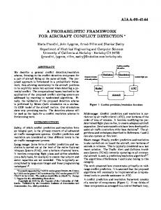
which relates the reflection coefficients seen looking into port 1 (Γ1 ) and out of port 2 (Γ2 ) of a two-port device within a network (see Figure 1). A. Coaxial cable For nominal (i.e., unfaulted) segments of the cable, one has S11 = S22 = 0, S12 = S21 ≡ S0 (l), where the dependence of the relevant S-parameters on the cable length l has been indicated explicitly for later convenience. Adopting the standard textbook model for a coaxial transmission line (see, for instance, [7], p. 551) one obtains S0 (l) = e−jk(ω)l , where √ k(ω)  ω μ0 d +

1 2 ln(b/a)



ωd jσc

(2) 

1 1 + a b

 .

(3)

In (3), a and b respectively denote the radius of the core and the (inner) radius of the shield, both of which are assumed to have a (finite) conductivity σc , while d denotes the permittivity of the insulator separating the two conductors, and μ0 is the vacuum permeability. We will also need the characteristic impedance of the cable, which is given by Z0 =

ln(b/a) k(ω) . 2π ωd

(4)

The above formulation relates the key cable parameters (S0 and Z0 ) directly to the “constitutive” parameters (σc and d ), and is therefore preferable to the distributed RLCG parameter model that is more commonly found in textbook treatments.

d ZF

Z0 Γ1

Fig. 1.

where ΓS = (Z0 − ZS )/(Z0 + ZS ) accounts for the port impedance mismatch, tM represents the one-way internal delay, and G is the gain factor used to account for possible calibration issues. The key parameters for the TDR unit are thus seen to be the source impedance ZS , the internal delay tM , and gain factor G.

Z0 Γ2

A constant-impedance model for a chafed cable segment.

D. Model synthesis B. Chafing fault A simple yet accurate model for the S-parameters of a chafed coaxial cable is now presented using an approach that is generalizable to other types of wiring. The situation of interest is depicted in Figure 1, where a segment of length d is chafed on a coaxial cable with characteristic impedance Z0 . The chafed segment is modeled as having a constant (i.e., z- and ω-independent) characteristic impedance ZF . The Sparameters for this segment are readily found to be: Γ2 (e−jω2(d/vp ) − 1) , 1 − Γ22 e−jω2(d/vp ) (1 − Γ22 )e−jω(d/vp ) = , 1 − Γ22 e−jω2(d/vp )

S11 = S22 =

(5)

S21 = S12

(6)

where Γ2 = (Z0 − ZF )/(Z0 + ZF ), and vp is the velocity of propagation through the chafed segment. We must next relate the hitherto unknown parameters ZF and vp to the geometry of the chafe. This can be accomplished by modeling the chafe as a rectangular section of removed shielding having a width w, and building a look-up table that maps w to ZF and vp . We have found that this simple rectangular geometry is remarkably accurate for modeling practical chafes, which are typically elliptical in shape. For the theoretical underpinnings and the numerical implementation of this approach, the reader is referred to [8]1 . C. TDR hardware A general model for the TDR hardware is shown in Figure 2. In this figure, the “down-stream network” represents any wiring system that is defined by a characteristic impedance Z0 and a reflection coefficient Γ0 at the system input. The goal is to determine the experimentally measured voltage VM in terms of the TDR source voltage VS . Good models for TDR hardware should incorporate three practical effects: (1) the frequency-dependent impedance mismatch between the source and the cable, (2) a measurement delay time needed to account for signal propagation within the TDR unit, and (3) a gain factor to account for a typically small miscalibration between the modeled and measured TDR response voltages. The equation below for the net transfer function captures these effects:   ΓS + Γ0 −j2ωtM G VM 1+ , (7) = e H(ω) = VS 2 1 + ΓS Γ0

The pieces discussed separately above are now put together to obtain the system model shown in Figure 3. The model is analyzed from right to left, starting with the load reflection coefficient ΓL = (ZL − Z0 )/(ZL + Z0 ). By repeated application of equation (1), we obtain Γ2 = S02 (l2 )ΓL , S12 S21 Γ2 , Γ1 = S11 + 1 − S22 Γ2 Γ0 = S02 (l1 )Γ1 ,

(8) (9) (10)

where S0 (l) is given in (2), and Sij are given in (5) and (6). Inserting these equations into (7), we obtain an analytical relationship between the TDR input and output signals, which explicitly contains the various physical system and fault parameters discussed above. (The derivation is straightforward, but the result is too unwieldy to include here.) Rewriting (7) in the time domain2 , we have  t vM (t) = h(t − t ; θ) vS (t ) dt , (11) 0

where the dependence of the impulse response h on the set θ of key model parameters has been indicated to motivate 2 In taking the inverse Fourier transform of H(ω) to obtain h(t), one must respect the frequency dependence of the various S-parameters and impedances in the model, which has been suppressed throughout for notational simplicity.

TDR hardware

VM e−jωtM

ZS

+

Γ0 =

VS

V− V+

down-stream network Z0 =

−

Fig. 2.

V+ I+

=

V− I−

TDR hardware model.

TDR Hardware

z = 0+

coax

chafe

coax

l1

d

l2

ZL

 V + (ω, 0) TDR Hardware

Γ0

S0 , Z 0

Γ1

S

Γ2

S0 , Z0

V − (ω, 0)

1 Note

the method presented in [8] assumes vp √ is equal to the nominal velocity of propagation on the cable, which is  1/ μ0 d . While this is not theoretically true, the assumption seems to work reasonably well in practice for the small chafe faults considered in this paper.

Fig. 3.

S-parameter representation of a chafed coaxial cable.

ΓL

ZL

the discussion in §III. Typically, equation (11) is computed numerically using the Fast Fourier Transform (FFT) algorithm. We note in passing that this modeling approach can be generalized readily to a cable with chafes (or other kinds of faults) at multiple locations, and in fact to arbitrary wiring networks. Most importantly, as the number of wiring and interconnect components grows, the computational effort needed to evaluate the model grows only linearly, and the memory resources needed stays roughly fixed. III. P ROBABILISTIC INVERSION A. Bayesian framework In this section, a probabilistic framework is presented for inferring the fault parameters from measured TDR data. Starting with a sampled version of (11), the measurement process is modeled in the usual way as y = F (x; θ) + ν,

(12)

where x ∈ Rn is the interrogation signal injected by the TDR unit into the cable under test, θ ∈ Rm is the set of unknown model (i.e., system and fault) parameters, the function F (x; θ) : Rn × Rm → Rn represents the forward model, ν ∈ Rn is a vector of additive random measurement noise, and y ∈ Rn is a time series of voltage samples forming the measured TDR signal. Two probability distributions are now introduced for the construction of a Bayesian inversion framework: (1) the prior distribution Prob(θ), which describes our state of knowledge regarding the unknown model parameters before any measurements are made, and (2) the likelihood distribution Prob(y|θ), which specifies the probability of observing a particular measurement for a given set of model parameters. Bayes’ theorem then gives the posterior distribution for θ in the form [4] Prob(θ|y) = 

Prob(y|θ) Prob(θ) . Prob(y|θ ) Prob(θ ) dθ

(13)

The maximum a posteriori estimate θ∗ is found by solving the optimization problem maximize Prob(θ|y).

(14)

Furthermore, the shape and the spread of the posterior distribution around θ∗ indicate how confident we are in this estimate. There are two typical approaches to quantifying this shape for general distributions like Prob(θ|y), which depends heavily on the nonlinear forward model (among other things). The first is to assume the distribution is approximately Gaussian around the optimal estimate θ∗ , and to use the inverse of the Hessian of − log Prob(θ∗ |y) as an approximation for the covariance matrix which quantifies the spread of the distribution [4, Ch. 3]. The second approach relies on the remarkable fact that one can sample random vectors directly from the posterior distribution Prob(θ|y), and use the spread of the samples to quantify the distribution shape, without making any additional Gaussian assumptions. This is the approach we take up in the next section.

B. Markov-Chain Monte Carlo estimation Finding the optimal estimate and quantifying the uncertainty associated with it are computationally challenging tasks when the forward model F is nonlinear in θ, as in the present case. Furthermore, in cases where the forward model is an algorithm (rather than a closed-form expression), it can be prohibitively expensive to compute the gradient and the Hessian of the cost function, which are needed to solve the optimization problem (14) using traditional methods. Thus, a natural approach for this type of problem is the application of Markov-Chain Monte Carlo (MCMC) methods to obtain a set of random samples drawn directly from the posterior distribution, which are used to estimate the desired quantities by applying the law of large numbers. The underlying premise for this approach is that, for sufficiently large N , a set of samples θi ∼ Prob(θ|y),

i = 1, 2, . . . , N,

(15)

adequately captures the essential features of the posterior distribution. Specifically, the sample θk that maximizes the posterior distribution provides us with a globally optimal estimate, while the spread of the N samples around θk may be taken as a measure of our uncertainty about this estimate. There are many different MCMC-based algorithms one might implement to achieve the above sampling. The results presented in §IV were obtained using a relatively new method called nested sampling. This algorithm is a natural fit for solving the estimation problem posed by equations (13) and (14), while also estimating other relevant quantities such as the integral in the denominator of (13), which can be used for model selection (i.e., choosing the best among competing forward-modeling schemes). Like many other MCMC methods, this one also tends to be slow: it took around 8 hours to solve the estimation examples discussed in §IV on a 32-bit 1.8-GHz Linux PC. The interested reader is referred to [4] for details on the nested-sampling algorithm. IV. R ESULTS This section presents our results on system parameter estimation and chafing fault detection for a 7-m long RG58 coaxial cable with an open load condition (i.e., ZL = ∞). Laboratory measurements were obtained using an Agilent 54754A digital TDR unit. The elements of the measurement noise vector ν were assumed to be independent and identically distributed Gaussian random variables with zero mean and a standard deviation of 1 mV, a value roughly equal to the worst-case residual error between the measured data and the optimal model fit. Finally, please note the results presented here are dependent on the assumption that the total cable length is known exactly, which may not be true in many practical settings. A. Estimating the system parameters Recalling the development of §II, the key system parameters that should be inferred from data are the metallic conductivity and the dielectric permittivity of the coaxial cable, as well as the port impedance, internal delay, and gain of the TDR unit.

95% Confidence Ellipse & Posterior Samples 2.24

2.2395

2.239

d

2.2385

2.238

2.2375

2.237 3.02

3.03

3.04

3.05

σc

3.06

3.07

3.08

3.09 7

x 10

Fig. 4. The optimal estimate and the confidence ellipse for the coaxial cable model parameters. The star marks the most probable estimate, while the ellipse encloses 95% of the samples drawn from the posterior distribution.

Although nominal values of σc and d are typically supplied by the cable manufacturer, the parameters of a particular cable may deviate appreciably from the “batch” values, and therefore it is advisable to infer them instead from measured data. The same argument holds for the TDR hardware parameters as well. Thus, for the first inversion problem to be solved, one has θ = (σc , d , ZS , tM , G). Figure 4 shows the optimal estimates for σc and d , along with the estimation uncertainty (specified as a 95% confidence ellipsoid) obtained with our inversion procedure. The optimal estimates ± one standard deviation were: conductivity σc = 3.054 ± 0.017 × 107 S/m, relative permittivity d = 2.2384 ± 0.0006, source impedance ZS = 48.97 ± 0.02 Ω, delay tM = 0.2858 ± 0.0044 ns, and system gain G = 1.00774 ± 0.00008.

B. Estimating the fault parameters The system parameters estimated above are now treated as fixed, and the fault parameters are estimated from measured TDR data with a single chafe at a distance of 6 m from the source. Thus, for this second inversion problem to be solved, one has θ = (w, d, l1 ) (i.e., the width, the length, and the location of the chafe). The results of the MCMC estimation scheme are presented in Figure 5. The distance to fault was estimated to be 6.016±0.002 m, while the length and the width of the chafe are estimated to be 14 ± 3 mm and 2.8 ± 0.1 mm, respectively. The true fault parameters as measured in the lab with a tape measure for distance and calipers for length and width were in good agreement with these estimates (i.e., were within the derived confidence ellipsoid). With all the key model parameters inferred from data, we now use the optimal parameter estimates and the known source voltage profile vS (t) to compute the model-predicted TDR signal, vM (t). The result presented in Figure 6 shows near perfect agreement with the laboratory measurement.

Fig. 5. The optimal estimate and the confidence ellipsoid for the chafing fault parameters. The star marks the most probable estimate, while the ellipsoid encloses 95% of the samples drawn from the posterior distribution.

secondary chafe reflection

0.4

0.395 0.35

v(t) (V)

3.01

input signal

0.39

measured response 0.3

model fit

0.25

primary chafe reflection

90.5

91

91.5

0.214 0.212 0.21 0.208

0.2

70.5 20

40

60

80

100

71 120

71.5 140

72 160

t (ns) Fig. 6. Model fit to the measured TDR signal using the optimal estimate for θ. The fit captures the variation in the measured signal to within 1 mV, and includes both the primary and the secondary reflections from a single chafing fault.

R EFERENCES [1] K. R. Wheeler, D. A. Timucin, I. X. Twombly, K. F. Goebel, and P. F. Wysocki, “Aging aircraft wiring fault detection survey,” NASA Ames Research Center, http://ti.arc.nasa.gov/m/pub/1342h/1342 (Wheeler).pdf, Tech. Rep. 1342, June 2007. [2] L. Griffiths, R. Parakh, C. Furse, and B. Baker, “The invisible fray, a critical analysis of the use of reflectometry for fray location,” IEEE Sensors J., vol. 6, no. 3, pp. 697–706, June 2006. [3] E. Song, Y.-J. Shin, P. E. Stone, J. Wang, T.-S. Choe, J.-G. Yook, and J. B. Park, “Detection and location of multiple wiring faults via timefrequency-domain reflectometry,” IEEE Transactions on Electromagnetic Compatability, vol. 51, no. 1, pp. 131–138, February 2009. [4] D. Sivia and D. Skilling, Data Analysis, 2nd ed. Oxford University Press, 2006. [5] R. Collin, Foundations for Microwave Engineering, 2nd ed. New York: McGraw-Hill, Inc., 1992. [6] R. Ludwig and P. Bretchko, RF Circuit Design Theory and Applications. Prentice Hall, 2000. [7] J. A. Stratton, Electromagnetic Theory. New York: McGraw-Hill, 1941. [8] M. Kowalski, “A simple and efficient computational approach to chafed cable time-domain reflectometry signature prediction,” in Annual Review of Progress in Applied Computational Electromagnetics Conference. ACES, March 2009.