[14] Robbert van Renesse, Kenneth Birman, and Werner. Vogels. Astrolabe: A robust and scalabel technology for distributed system monitoring, management, ...
A Model-Driven Approach to Distributed Information Management Jin Liang∗, Xiaohui Gu†, Klara Nahrstedt∗ ∗
Dept. of Computer Science University of Illinois at Urbana-Champaign Urbana, IL 61801 {jinliang, klara}@ cs.uiuc.edu
Abstract
Dept. of Distributed Computing IBM T.J. Watson Research Center Hawthorne, NY 10532 {xiaohui}@ us.ibm.com
To properly adjust its behavior, however, an autonomic system must be able to promptly “sense” the changes in its environment. Thus, one fundamental building block in any autonomic distributed system is an efficient distributed information management service [14, 16], which can resolve queries about the distributed system. A common set of queries include multi-attribute range queries such as “find 10 machines that have at least 20% free CPU time, 20MB memory, and 2G disk space”. The goal of this research is to design and build a distributed information management system that can answer multi-attribute range queries about large-scale distributed systems.
In this paper, we present a model-driven distributed information management system called MDIM that can resolve multi-attribute range queries about large-scale networked systems. Different from previous work, MDIM can adaptively configure its information collection and query resolution operations based on a dynamically maintained information model. The information model captures both statistical information query patterns (e.g., frequently queried attributes, frequently queried value ranges) and information attribute properties (e.g., node attribute distributions). Thus, MDIM can better scale to large numbers of system nodes and attributes than static schemes by intelligently minimizing monitoring overhead. We have implemented a prototype of MDIM and evaluated its performance using both extensive simulations and micro-benchmark experiments. Our experimental results show that MDIM always produce much smaller system overhead than static monitoring schemes. More importantly, when system conditions or query patterns change, MDIM can adaptively reconfigure itself in response to the changes.
1
†
However, it is challenging to provide scalable and efficient information management service for dynamic, largescale distributed systems. On one hand, we need upto-date information about the current system to provide accurate query answers. On the other hand, the system can consist of large numbers of geographically dispersed nodes (e.g., World Community Grid [2]) and each node can be associated with many dynamic attributes (e.g., CPU load, memory space, disk storage). Obtaining accurate information about all nodes with all their attributes would inevitably involve high system overhead [16]. To resolve a query, there are two principle approaches for acquiring necessary attribute data: (1) information push where each node periodically reports its current attribute data to the system; and (2) information pull where the system dynamically probes a subset (or all) of the nodes to resolve the query. The relative merit of each approach depends on both query patterns (e.g., query rate, query attributes) and system conditions (e.g., attribute value distributions). For example, when the query arrival rate is high and different queries ask the same set of attributes, the push approach is more efficient since its cost is amortized among many queries. However, when the query arrival rate is low and different queries ask different set of attributes, the pure push solution can become inefficient since most pushed data are only used by a few queries. In contrast, the cost of pull approach is related to the query arrival rate. When there are few
Introduction
Large-scale distributed computing systems such as computational grids [8] and open network platform [12] have become increasingly important for various application domains such as cancer study, drug discovery, scientific computation, and Internet service provisioning. As these systems continue to grow, how to efficiently manage such large-scale distributed systems has become a challenging task. Inspired by how human nervous system reacts to external changes, the autonomic computing paradigm has recently been proposed as a viable approach to building self-managed distributed systems [11]. An autonomic system can dynamically adjust its own behaviors to adapt to environmental changes, so that a high level management goal of the system is always achieved. 1
queries, very little pull cost is incurred. However, when there are a lot of queries, excessive overhead might be incurred. In a dynamic distributed system where query patterns and system conditions can change over time, any static solution (i.e., statically configured push/pull operations) can fall short. Thus, we propose a new modeldriven approach to distributed information management, which can adaptively configure its information collection and query resolution operations based on current system conditions and query patterns. In this paper, we present the design and implementation of the first model-driven distributed information management system called MDIM. The goal of MDIM is to resolve multi-attribute range queries for large-scale distributed systems with minimum cost. To achieve this goal, MDIM dynamically estimates the current query patterns and adaptively adjusts its operations to minimize the total system cost (i.e., combined push and pull cost). The system dynamically selects a subset of nodes to periodically push a subset of all attributes. The subset of nodes and attributes are selected so that most queries can be resolved by the pushed data. For the queries that cannot be resolved by the push data, the system invokes a pull operation to acquire necessary information to resolve the queries. Specifically, this paper makes the following contributions,
interval for each pushed attribute. We design and implement a set of configuration algorithms that can optimally adjust the three system parameters based on the current information model. • We have implemented a prototype of the MDIM system. We conduct both simulations and microbenchmark experiments on 280 PlanetLab [12] nodes. Our experiments show that MDIM can achieve much lower overhead than static solutions (e.g., pure push or pull). More importantly, when system conditions or query patterns change, MDIM can adaptively reconfigure itself in response to the changes. The rest of the paper is organized as follows. Section 2 presents the overview of our model-driven distributed information management (MDIM) system. Section 3 presents the design and implementation of MDIM. Section 4 presents experimental results. Section 5 discusses related work. Finally, the paper concludes in Section 6.
2 Overview of MDIM In this section, we present an overview of the MDIM system including its information query model, its configurable system architecture, its information model that serves as the knowledge base for automatic selfconfiguration, and major configuration problems addressed by MDIM.
• We propose a new model-driven approach to distributed information management, which enables MDIM to automatically configure itself based on a dynamically maintained information model. The information model serves as the knowledge base for MDIM to intelligently configure its monitoring operations to adapt to dynamic query patterns and distributed system environments.
2.1 Query Model
Let us consider a federated distributed system that has N system nodes to be monitored. Each node is associated with a set of attributes such as CPU load and number of • We design and implement an information model disk accesses, which is denoted by A = {a1 , ..., a|A| }. that captures system attribute distributions and three Each attribute is represented by an attribute name (e.g., important query patterns: (1) frequently queried CPU, memory) and value (e.g., 10%, 20KB)1 . MDIM attributes; (2) frequently queried range values; and supports multi-attribute range queries which can be used (3) frequent staleness constraints (i.e., the attribute by many applications such as distributed resource discovvalue should be no more than a certain time old). ery. Each query is in the form of q = (a1 ∈ [l1 , h1 ]) ∧ The information model provides important guidance (a2 ∈ [l2 , h2 ])... ∧ · · · (ak ∈ [lk , hk ]), where li and for MDIM to achieve optimal trade-off between the hi are the desired lower bound and upper bound for ai , push and pull operations for minimum monitoring respectively. For example, the query “find a machine that overhead. Thus, MDIM can achieve scalability with has at least 20KB memory and 10% free CPU time” can regard to both nodes and attributes. be represented as q = (cpu ∈ [10%, ∞)) ∧ (memory ∈ • We identify a set of configuration parameters that [20KB, ∞)). Each query can also specify the number of can be used as tuning knobs by an autonomic dis- nodes that are needed. The query answer should return tributed monitoring system. Specifically, MDIM the specified number of nodes, each of which satisfies can dynamically configure (1) a subset of attributes the k attribute requirements. The default value of the that should be pushed; (2) push threshold values of node number is set as one. Finally, each query can also 1 Unless specified otherwise, we use a to represent both name and each pushed attribute, which determines the subset i of nodes that need to push their data; and (3) update value of the attribute. 2
specify a staleness constraint Ti on a required attribute ai , which means the attribute value used to resolve this query should be no more than Ti seconds old. Applications can have different staleness constraints on different attributes depending on the properties of the applications and attributes. For example, one query may require some nodes that have a certain amount of free CPU time, and the measurement data should be within the last 30 seconds; while another query may require some nodes to have a certain amount of disk space, as long as the measurement data are within the last 5 minutes.
2.2
where each node periodically reports its current attribute data to an information repository; and (2) information pull where the system dynamically probes a subset (or all) of the nodes on-demand to resolve the query. The relative merit of each approach depends on information query patterns and current system conditions. Thus, to leverage the benefits of both approaches, MDIM adopts a configurable monitoring architecture illustrated by Figure 1. MDIM adaptively combines push and pull operations based on a dynamically maintained information model summarizing current query patterns and system conditions. We deploy a monitoring daemon on each node, which is capable of periodically pushing the attribute data on that node to a system manager every T seconds, or respond to a resource probing message with the current attribute data. Here T is called the push interval. The system manager can be viewed as the super nodes in the distributed system, which is responsible for maintaining aggregated view of the system and resolving queries. We can deploy multiple system managers in the system based on the system size and query load conditions. Each monitoring daemon is configured to periodically push its attribute data to the system manager. However, not all attributes on the nodes are pushed, and not all nodes push their attribute data. The push interval can also be different for different attributes. As a result, only the attribute data that are likely to be queried are pushed. Because not all attribute data are periodically pushed, some queries may not be able to be locally resolved at the system manager. For example, a query may want to find a node with a certain free disk space, but the free disk attribute is currently not being pushed since only a few queries include the free disk attribute. At this time, a resource pull operation is invoked to locate a node with enough disk space. Figure 1(b) shows the query resolution flow in MDIM. When a query arrives, the system manager first checks if all the attributes in the query are within the subset of popular attributes being pushed (denoted as A∗ ). If so, it checks if the required attribute ranges are within the push threshold. Next, it checks if the staleness constraint for the attributes are larger than the push intervals. If all of the above are satisfied, then the query is locally resolved. Otherwise, dynamic pull is invoked for its resolution. There could be different ways for the system manager to pull the necessary attribute data. For example, it can randomly select a subset of nodes and send probe messages to these nodes (random sampling). Or it can dynamically create a monitoring tree [9] and propagate the probe message down the tree. For our model based approach, we are concerned with the overhead for each pull operation, rather than how the pull operation is executed. As a result, we assume to resolve a query by pull, on average the system manager needs to contact n nodes with 2n probing messages (i.e., both probes and replies).
Configurable System Architecture Periodic Push On Demand Probe System Manager
Query
Info Repository
node 1
cpu 65%, ...
node 3
cpu 30%, ...
...
�
� �
�
� �
...
�
node N ....
node 1 � �
� �
�
� �
�
node 2
�
�
node 5
� �
�
� �
�
� �
�
�
node 3
node 4
(a) MDIM system architecture.
query arrival
attributes are in A*
N
Y lower bound within threshold
N
dynamic probe
Y staleness constraint satisfied
N
Y local resolve (b) Query resolution flow.
Figure 1: MDIM model and query resolution To resolve a query, there are two different approaches to acquire necessary attribute data: (1) information push 3
CDF
are periodically reported to the system manager. Since those attributes are shared by many application queries, it is more efficient to report them to the system manager than perform a pull operation for each individual query. Thus, the first task in our model inference is to identify those popular attributes among all current queries. Frequently queried range values. Besides to select most popular attributes to push, we can further reduce the monitoring overhead by filtering out unqualified attribute values. For example, if most queries on CPU time require a node to have at least 20% free CPU time, then the nodes with less than 20% CPU time do not need to push their attribute data, because it is unlikely that these nodes will satisfy a query on free CPU time. Thus we can configure the monitoring daemons on different nodes to push their free CPU time only if they have more than 20% free CPU time. The intuition is that heavily loaded nodes do not need to push their up-to-date attribute value since they are unlikely to satisfy the range query requirements. Thus, for each frequently queried attribute, we configure the monitoring daemon on each node with a subrange [li , ∞), so that only those attribute values that fall into this range are periodically report to the system manager. The range lower bound li is called the push threshold for the attribute. By properly setting the push threshold, we can filter out many unnecessary information push without significantly decreasing the query hit ratio (i.e., percentage of queries can be resolved by the push data). Figure 2 illustrates the problem of push threshold selection for one attribute. The solid line is the cumulative distribution function (CDF) of an attribute a1 across all N nodes, and the dashed line is the CDF of the lower bound on the attribute for all the queries. As the figure shows, 90% of the queries require the attribute to be greater than l, and only 74% of the nodes satisfy this requirement. This means if we configure the nodes to push their attribute data if the attribute value is greater than l (i.e., set the push threshold to be l), 74% of the nodes will need to push their attribute data and 90% queries can be resolved by the push data. However, 65% of the queries require the attribute to be greater than l0 , and only 20% of the nodes satisfy the requirement. Therefore if we increase the push threshold from l to l0 , then only 20% of the nodes need to push their attribute data, but 35% of the queries will involve resource pull. Thus, the second task in our model inference is to keep track of query requirement distributions and attribute value distributions for configuring proper push thresholds. Frequent staleness constraints. The last query pattern maintained by MDIM keeps track of the frequent staleness constraints among recent user queries. Depending on a particular application, the user may require the attribute data used for resolving his or her query should be no more than Ti for the attribute ai . This Ti is called the
1.0 0.8 Attribute Distribution Request Distribution
0.35 0.26 0.1
l
l’
a1
Figure 2: Push Threshold Selection for One Attribute. There are two ways to derive the value of n. First, if random sampling is used for probing, then from the node attribute distribution (as we will describe in Section 2.3), we can know the probability that a randomly selected node will satisfy the query. Suppose this probability is q, then on average 1q nodes need to be probed before the first node that satisfies the query is located. Alternatively the number n can also be derived empirically, based on previous probes. Since MDIM combines the push and pull approaches for monitoring, it has two kinds of system overhead, the push cost and the pull cost. The push cost is the amount of data periodically delivered from different nodes to the system manager over the network every time unit. It is determined by the number of nodes that periodically pushes the data, the push interval, and the packet size of each push message. The pull cost is the amount of data generated per time unit for pulling the attribute data, in response to queries that cannot be resolved by the system manager locally. It is determined by the arrival rate of such queries, the number of nodes n that need to be probed for each query, and the size of each probe and reply message.
2.3
Information Model
MDIM performs automatic self-configuration based on a dynamically maintained information model that captures both statistical query patterns and system attribute properties. Specifically, in the current MDIM prototype implementation, the information model keeps track of the following statistical information: Frequently queried attributes. Although system nodes can be associated with many attributes, it is likely only a subset of them are frequently queried by current applications. For example, in distributed applications where most computing jobs are CPU bound and there is little inter-node communication, it is likely that most queries will specify requirements on CPU resource, but not on network bandwidth. By keeping track of those popular attributes, MDIM can dynamically configure the monitoring daemons so that only most popular attributes 4
notation N A A∗ f1 T Ti∗ Ti S1 S2 λ n p1 li li∗ f2 p2 p3
2.4 Configuration Problems
meaning total number of nodes to be monitored set of all attributes subset of attributes to be pushed ∗ | fraction of pushed attributes f1 = |A |A| push interval optimal push interval for ai staleness constraint of a query size of push message size of probe message average query arrival rate avg. num. of probes for resolving a query % of resolvable queries using A∗ lower bound requirement for ai (optimal) push threshold ai % nodes in the push subspace % queries in the push subspace % queries satisfied by the push intervals
Based on the dynamically maintained information model, MDIM adaptively configure its monitoring daemons to achieve minimum monitoring overhead under current query patterns and system conditions. Specifically, MDIM addresses three configuration problems: (1) which attributes should be selected to report its up-to-date data?; (2) what push threshold should be used for each selected attribute?; and (3) what push interval should be employed for each selected attribute when its value is above the push threshold? Table 1 lists all the notations used by the following problem analysis. We define the push cost or pull cost as the size of total push messages or pull messages produced by the MDIM system per second. Problem 1: Popular attribute selection. When a query arrives, the system manager first checks whether the query can be resolved using its information repository consisting all the pushed data reported by different monitoring daemons. No pull cost is incurred if the query can be resolved by the push data, which is called a query hit. Otherwise, the system needs to invoke an on-demand probing protocol (e.g., [9]) to find enough nodes that satisfy the query. Suppose each monitoring daemon is configured to periodically push a subset A∗ of all attributes A (every T seconds) and the push message size is proportional to the number of attributes pushed. We ∗ | use f1 = |A |A| to denote the percentage of attributes that are pushed and S1 to define the size of a push message if all |A| attributes are reported. Thus, the push cost of the whole system can calculated by T1 N f1 S1 . Suppose the average query arrival rate is λ and on average we need to probe n nodes with 2n messages (probes and replies) in order to resolve a query that cannot be answered by the push data 2 . Let p1 denote the query hit ratio (i.e., the percentage of all queries that can be resolved using the push data). Let S2 denote the size of a probe message 3 . Thus, the pull cost of the whole system can be calculated by 2n(1 − p1 )λS2 . As a result, if only the attributes in A∗ are pushed, the total system cost is
Table 1: Notations.
query’s staleness constraint. In MDIM, each attribute sample data is associated with a time-stamp that indicates when the sample data is collected. For any attribute ai ∈ A∗ , it is likely that different queries may have different staleness requirements. As a result, the push interval (i.e., update period) of ai should be dynamically configured, so that the staleness constraint of most queries can be satisfied using the pushed attribute data, while for a small number of queries with stringent staleness constraint, pull operations are invoked to obtain more up-to-date attribute values on-demand. Attribute data distributions. In addition to the query patterns, our MDIM system also utilizes the node attribute distributions. Such distributions can be used for two purposes. First, when a query comes that needs to be resolved by probing, the node attribute distributions allow us to estimate the probing cost (i.e., the number of probes that will be generated). Second, when we configure the push threshold for the attributes to filter out unqualified nodes, we must compare the push cost reduction because of the node filtering, and the pull cost increase due to more probing operations. The push cost reduction can only be derived from the node attribute distributions. Since our system involves multiple attributes, we maintain multi-dimensional histograms to estimate the attribute distributions. Using histograms allow us to summarize the node attribute distributions in a concise fashion.
1 N f1 S1 + 2n(1 − p1 )λS2 . T
(1)
The selection of A∗ will affect the value of f1 and p1 , which can thus be viewed as one of the tuning knobs of the monitoring system. Thus, MDIM dynamically selects A∗ based on the current information model, so that the overall system cost in Equation(1) is minimized. 2 if part of the attributes specified by the query are pushed, the requirements on these attributes can be resolved to limit the scope of probing. 3 Since it is unlikely for a query to specify requirements on many attributes [3], we assume the message size for both probe and reply is S2 , which is a constant much smaller than S1 .
5
interval Ti∗ for each attribute ai ∈ A∗ based on the current queries’ staleness requirements, so that total system cost in Equation(3) is minimized.
Problem 2: Push threshold configuration. Assuming the subset A∗ has been selected, we can construct a |A∗ |dimensional space where each dimension is represented by one attribute. If we select a push threshold li∗ for each attribute ai , then the set of push thresholds define a subspace {(a1 , a2 , · · · , a|A∗ | )|ai ≥ li∗ , 1 ≤ i ≤ |A∗ |} in the whole |A∗ |-dimensional space. We say a node is “covered” by the subspace, if its current value for each attribute ai ∈ A∗ is greater than the corresponding push threshold. We say a query is “covered” by the subspace, if all the nodes that satisfy the query (called the answer set of the query) are covered by the subspace 4 . If we configure a node to report its attribute data if and only if it is covered by the subspace, then for all the queries covered by the subspace, they can be locally resolved by the system manager. Suppose f2 percent of the system nodes are covered by the subspace defined by the push thresholds, then the push cost of the system is reduced to T1 f2 N f1 S1 since not all nodes report the selected A∗ attribute data. Correspondingly, if p2 percent of the queries (among those that only specify attributes in A∗ ) are covered by the subspace, then a total of (1 − p1 p2 ) percent of all queries need to be resolved by information pulling, and the pull cost is 2n(1 − p1 p2 )λS2 . As a result, the total system cost is 1 f2 N f1 S1 + 2n(1 − p2 p1 )λS2 . T
3 Design and Implementation We now present the design and implementation of the MDIM automatic configuration algorithms that strives to achieve improved scalability with respect to both nodes and attributes by observing both query patterns and attribute distributions.
3.1 Popular Attribute Selection The goal of push attribute selection is to select a subset A∗ of attributes from the attribute set A, so that the total system cost is minimized, when only the attributes in A∗ are periodically pushed. According to Equation(1), A∗ can affect the packet size (f1 percent of a full push message) of a push message and the percentage p1 of queries that can be locally resolved by the system manager. Larger A∗ implies a larger push packet size and a smaller percentage of queries that need to invoke pull operations, while smaller A∗ implies smaller push packet size but larger number of queries that need to be resolved by pull. Thus, the selection A∗ represents the trade-off between the push cost and pull cost. Our goal is to select a proper subset A∗ such that the combined push and pull cost is minimized. To quantify the relative merit of pushing a subset of attributes, we group the queries based on the subset of attributes specified in the query. For example, we use Ai = {a1 , a2 } to represent all queries that specify requirements on attributes a1 and a2 . For each subset Ai , we can compute a query frequency, denoted by f req(Ai ), which means the percentage of all queries that are represented by Ai . If Aj ⊆ Ai , then when we push the attributes in Ai , the queries represented by Aj can also be resolved locally by the system manager. Therefore, we definePthe cumulative query frequency of Ai as f req 0 (Ai ) = Aj ⊆Ai f req(Aj ), which indicates the percentage of queries that the system manager can locally resolve, if the attributes in Ai are pushed. Given the above, we can define the relative cost reduction of a i| subset Ai to be 2n · f req 0 (Ai )λS2 − T1 N |A |A| S1 , i.e., the amount of pull cost saved minus the additional push cost incurred, if Ai is pushed. Our algorithm for selecting the push attributes, shown by Figure 3, works as follows. Let C denote the collection of query instances, each of which consists of an attribute subset Ai . Initially, we set A∗ to be empty, which means no attribute is pushed. Thereafter, we repeatedly select the subset Ai with the largest cost reduction, and add Ai
(2)
The configuration of li∗ , 1 ≤ i ≤ |A∗ | will affect the values of f2 and p2 . Thus, the goal of MDIM is to select a proper push threshold li∗ for each attribute ai ∈ A∗ , so that the total system cost in Equation (2) is minimized. Problem 3: Push interval selection Suppose for each selected attribute ai ∈ A∗ , the push interval is set to be Ti∗ . Then, the push cost for attribute ai is S1 1 Ti∗ f2 N |A| . Thus, the total push cost for all selected P 1 S1 attributes is T ∗ f2 N |A| . Suppose under the above ai ∈A∗
i
configuration, p3 percent of the queries (among the p2 p1 λ queries that specify attributes in A∗ and are covered by the subspace defined by the push thresholds) can satisfy their staleness constraints. Then a total of (1 − p3 p2 p1 )λ queries need to invoke pull operations whose cost is 2n(1 − p3 p2 p1 )λS2 . Thus, the total system cost is X ai ∈A∗
(
1 S1 ) + 2n(1 − p3 p2 p1 )λS2 f2 N ∗ Ti |A|
(3)
The value of Ti∗ will affect the push cost and p3 . Larger Ti∗ means lower push cost but lower p3 implying higher pull cost. Thus, MDIM needs to properly configure a push 4 Here we only consider the queries that specify requirements on the attributes in A∗ . If a query specifies attributes not in A∗ , then it will always involve probing operations.
6
a2
AttributeSelection(T, N, A, S1 , S2 , n, λ) 1. let f1 = p1 = 0, and A∗ = ∅ 2. compute min cost using Equation(1) 3. let C = {Ai ⊆ A|f req(Ai ) > 0} 4. while C 6= ∅ do 5. for each Ai ∈ C compute f req 0 (Ai ) 6. select Ai from C that has the largest cost reduction. 7. if the cost reduction of Ai is negative then break i| 8. f1 = f1 + |A |A| 9. p1 = p1 + f req 0 (Ai ) 10. compute min cost using Equation(1) 11. A∗ = A∗ ∪ Ai 12. for each Aj ∈ C set Aj = Aj \Ai 13. merge duplicate subsets in C 14.return A∗
* +
* + * + * *+ + ** * + + + *
*
l’2 +
l2
queries nodes
l1
l’1
a1
(a) Two-dimensional subspace selection
a2 * +
queries nodes
+
q’ * *
*
Figure 3: Push attribute selection algorithm.
+
l2
+ +
*
q
* l1
∗
to A . The attributes in Ai are removed from all other subsets in C. This may create duplicate subsets in C. For example, after the attributes in Ai = {a1 , a2 } is removed, the two subsets {a1 , a3 } and {a2 , a3 } will be the same as each other. These subsets are then merged, and the cumulative query frequency is recomputed. The above process is repeated, until either all attributes have been added to A∗ , or the addition of a new attribute subset would lead to increased total system cost. To implement the algorithm, we keep a moving window of historical queries that the system manager has received. We also keep a moving average of p1 , the percentage of queries that only specify attributes in A∗ . Whenever the observed p1 is significantly different from the value predicted by our model, a reconfiguration is triggered. We now analyze the computational complexity of the algorithm. In the worst case, the while loop at line 4 will be executed |C| times. For each loop, line 5 will take O(|C|2 ) time because every pair of subsets need to be compared for inclusion test. The inclusion test for two subsets takes O(k 2 ) time, assuming k is the maximum number of attributes in a query. As a result, the worst case time complexity of the algorithm is O(|C|3 k 2 ).
3.2
*
+
* +
a1
(b) Query positioning
Figure 4: Subspace selection
{(a1 , a2 )|a1 ≥ l1 ∧ a2 ≥ l2 }. One query needs to be resolved by pull, because it is not covered by the subspace. However, if we set the push threshold to be l10 and l20 , then five nodes do not need to push their data, and three queries need to be resolved by pull. In the above description, we assume that each query has all |A∗ | coordinates, which means it specifies requirements on each attribute ai ∈ A∗ . In reality, a query may only specify a subset of the attributes in A∗ . At this time, we need to decide where in the |A∗ |-dimensional space this query is placed, so that our subspace selection algorithm can correctly classify it as locally resolvable or not. We call this procedure the “positioning” of a query. We now use an example to illustrate the positioning procedure shown by Figure 4(b). The figure shows a two dimensional space (i.e., A∗ = {a1 , a2 }) and a query q = (a1 ≥ l1 ). One intuitive way to place the query in the two dimensional space is to rewrite the query as q 0 = (a1 ≥ l1 ∧ a2 ≥ 0). As a result the query locates on the a1 axis. This, however, does not make use of the (aggregate) information that we may have about the system nodes, such as the distribution of the nodes. For example, if we know in Figure 4 that among the nodes that satisfy a1 ≥ l1 , the smallest a2 value is l2 , then we can rewrite the query as q 00 = {a1 ≥ l1 ∧ a2 ≥ l2 }. This does not change the set of nodes that satisfy the query. However, it does affect the classification of queries as locally resolvable or not. If the push attributes for a1 and a2 are set to l1 and l2 , respectively, q 00 is covered by the
Push Threshold Configuration
In section 2.4, we formulate the push threshold selection problem as selecting the multi-dimensional subspace that covers the optimal set of nodes and queries. Figure 4(a) shows the subspace selection problem in two dimensional space. Each star in the space corresponds to a query, and each plus sign corresponds to a node. From the figure we can see, if we set the push threshold for a1 and a2 to be l1 and l2 , respectively, one node does not push its attribute data because it is not covered by the subspace 7
subspace, while q 0 is not. Using the (conditional) attribute distribution, we can place the queries more accurately.
PushThresholdSelection(T, N, A, S1 , S2 , n, λ, A∗ ) 1. let li∗ = 0, 1 ≤ i ≤ |A∗ | and f2 = p2 = 1 2. compute min cost according to Equation(2) 3. let B and B 0 be the bins for nodes and queries 4. while B 6= ∅ do 5. select ai that has the largest cost reduction. 6. if the cost reduction is < 0 then break 7. increase li∗ to li∗ + δ 8. remove all nodes and queries not covered by {li∗ } 9. reduce the cost reduction from min cost 10.return {li∗ }
Query positioning requires us to run the queries against the node distribution. We use multi-dimensional histograms to estimate the distribution of the nodes and queries 5 . Since the dimension might be high, we only keep the bins that are non-empty. Suppose all the attribute values are normalized to [0, 1.0], and the bin size for each dimension is δ. Let B be the list of non-empty bins for the node attribute distribution. Each bin bi ∈ B is described by a tuple of |A∗ |+1 fields. The first |A∗ | fields define the bin, and the last field is the percentage of nodes in the bin. For example, b = (v1 , v2 , · · · , v|A∗ | , 0.1) means 10% of the machines have attribute ai ∈ [vi , vi +δ), 1 ≤ i ≤ |A∗ |. Similarly, let B 0 be the set of bins for the queries. B and B 0 are bounded by the number of nodes in the system and the number of historical queries that we keep for estimating query patterns, which should be much smaller than a complete multi-dimensional histogram. Suppose the current push threshold is li∗ for attribute ai . If we look at a particular attribute aj , and increase lj∗ to lj∗ + δ, we can compute how many nodes are removed from the subspace, and how many queries are removed the subspace. Suppose αj percent of the nodes are removed, and βj percent of the queries are removed, then the cost reduction for increasing lj∗ to lj∗ + δ is T1 αj N f1 S1 − 2nβj λS2 .
Figure 5: Push Threshold Selection Algorithm.
3.3 Push Interval Configuration The push interval configuration problem can be solved in a way similar to the push threshold configuration problem. Suppose we select a push interval Ti∗ for each attribute ai ∈ A∗ . The push interval controls how often a monitoring daemon reports the up-to-date value of the attribute to the system manager when the value is above the push threshold. Thus, push intervals can affect the system push cost. On the other hand, push intervals also affect how many queries can be resolved locally by the system manager satisfying their staleness constraints. Larger Ti∗ means the attribute is pushed less frequently. But it also means the pushed data is less likely to satisfy the staleness constraint of a query. The push interval configuration algorithm is very similar to the push threshold configuration algorithm, which are only briefly described as follows due to the space limitation. Basically, starting from the minimum push interval for each attribute, we repeatedly select an attribute ai and increase its corresponding push interval Ti∗ . ai is selected such that the increase of Ti∗ results in the largest cost reduction. The above process is repeated until either the increase of Ti∗ would lead to increased system cost, or when all the push intervals have reached their maximum values.
Our push threshold configuration algorithm is essentially a greedy algorithm illustrated by Figure 5. Initially, each push threshold li∗ is set to 0, which means every node periodically pushes its attributes. At each step, we select one attribute ai that has the largest cost reduction, increase the push threshold li∗ by a step size δ, and remove the nodes and queries that are not covered by the new subspace. This means less nodes need to periodically push their attribute data. On the other hand, more queries may need to be resolved by pull operations. The above process is repeated until the increase of any push threshold will cause the system cost to increase. In the algorithm, the while loop at line 5 executes at most |B| = O(N ) times. In each loop, line 6 needs to compute the cost reduction for each dimension ai . To do this, the number of 4 Experimental Evaluation nodes and queries that are removed when li∗ is increased ∗ 0 is computed, which takes O(|A |(|N | + |B |)) time. As In this section we present an experimental evaluation a result, line 6 takes O(|A∗ |(N + |B 0 |)N ) time. In of MDIM system. We first describe our simulation practice, N is often smaller than |B 0 | decided by the methodology and results, then present out prototype imnumber of queries. Thus, the computational complexity plementation of MDIM and our experiment results from of the algorithm is O(|A∗ | · N · |B 0 |). the PlanetLab [12] wide area network testbed.
4.1 Simulation Methodology
5 The query distribution can be estimated as queries arrive at the system manager. The node attribute data distribution can be obtained by infrequent aggregate queries over all the nodes, using methods such as those in [9].
Our simulation testbed consists of a query generator that can generate a range of different kinds of query 8
Total cost for different A* (single attribute queries)
workload, an information model that is a list of nonempty multi-dimensional histogram bins for the queries; and three modules that implement the three algorithms described in Section 3. For the second algorithm, we also have a node attribute generator. Unless otherwise specified, we assume the system size is N = 300, the push interval for the first two algorithms is T = 30 seconds, the total number of attributes is |A| = 50, the number of nodes to be probed for each pull is n = 10, the push packet size is S1 = 1000bytes and the probe packet size is S2 = 100bytes. Our parameters are chosen to represent a “typical” system. For example, for the CoMon [1] monitoring service currently running on the PlanetLab, each resource report contains more than 40 attributes, and has about 900 bytes. We use the system cost as defined in Section 2.4 as the main evaluation metric. For each experiment, we first generate a set of “training queries” (usually 2000 of them) using the query generator. The query arrival follows a Poisson process with arrival rate λ. We then run our algorithms to configure the system (i.e., to select push attributes, push thresholds, and push intervals). Next, we generate another set of “validation queries” according to the same model, and resolve the queries against our system configuration. The cost of the system for resolving the validation queries are computed. Each experiment is repeated 200 times, and the average cost is reported. We mainly compare the system cost of MDIM to that of the two static approaches, pure push and pure pull. In pure push-based systems, every node reports every attribute to the system manager. Thus the system cost is independent of the query arrivals. In pure pull-based systems, no proactive attribute push is involved. thus the system cost is proportional to the rate of query arrivals. We generate the queries and node attributes as follows. For each query, we first generate the number of attributes specified in the query. The number is uniformly distributed between 1 and k, where k is maximum number of attributes in a query. Next, the specified number of attributes are selected from A. The probability that a particular attribute is included in a query depends on the popularity of the attribute, which follows the Zipf distribution. After that, the lower bound on each attribute is generated. We assume that the value range of each attribute is divided into 20 equal sized bins (intervals). The probability that the lower bound for an attribute falls within a particular interval follows a particular distribution. The distribution that we used in our experiments is generated as follows. First, there is a most popular interval v. For the intervals whose values are larger v, their popularity follows a Zipf distribution with decreasing popularity as the interval value increases. Similarly, the popularity of the intervals smaller than v also follows a Zipf distribution, and the popularity decreases as the interval decreases. The node
12
λ=4 λ=5 λ=6
total system cost (KB/second)
11 10 9 8 7 6 5 4 0
10
20
30
40
50
number of most popular attributes included in A*
Figure 6: System cost for different number of attributes pushed (for single-attribute queries). Total cost for different query arrival rate 20
total system cost (KB/second)
18 16
k=1 k=3 k=5 pure push pure pull
14 12 10 8 6 4 2 0 1
2
3
4
5
6
7
8
9
10
query arrival rate (number of queries/second)
Figure 7: Multi-attribute queries. attribute data for the second algorithm are also generated using the same kind of distributions.
4.2 Simulation Results Figure 6 shows the system cost as a function of the subset of attributes being pushed. For this experiment we use single-attribute queries in order to see the tradeoff between the system cost and the subset A∗ . For single attribute queries, the popularity of the attributes is directly mapped to that of the queries. The x-axis shows the number of (most popular) attributes being pushed, and the y-axis shows the total system cost. We observe that for different query arrival rate λ, there is always an optimal number of attributes that lead to minimum system cost. For λ = 4, the optimal number is 9, and the minimal system cost is less than half of the cost when all attributes are pushed (pure push). When λ increases, slightly more attributes need to be pushed, and the optimal system cost also increases. However, the minimal system cost is always achieved when a subset of the attributes are pushed. Both pure push (when |A∗ | = 50) and pure pull (when |A∗ | = 0) will incur a much larger system cost. Figure 7 shows the system cost for multi-attribute queries. The system parameters are the same as the 9
Number of attributes selected for push
Total cost for push threshold selection
50
18
40
total system cost (KB/second)
number of attributes selected for push
45
20
k=1 k=3 k=5
35 30 25 20 15 10
14 12 10 8 6 4
5 0 1
16
k=1 k=3 k=5 pure push pure pull
2
2
3
4
5
6
7
8
query arrival rate λ (number of queries/second)
9
0 1
10
Figure 8: Number of attributes selected.
2
18 16
system cost (KB/second)
total system cost (KB/second)
6
7
8
9
10
20
k=1 k=3 k=5 pure push pure pull
14 12 10 8 6
12 10 8 6 4
2
2
2
3
4
5
6
7
8
query arrival rate λ (number of queries/second)
9
0 1
10
k=1 k=3 k=5 pure push pure pull
14
4
0 1
5
System cost for push interval selection
Total cost for push threshold selection
16
4
Figure 10: Cost when system nodes are heavily loaded.
20 18
3
query arrival rate λ (number of queries/second)
2
3
4
5
6
7
8
9
10
query arrival rate λ (number of queries/second)
Figure 9: Cost when system nodes are lightly loaded.
Figure 11: Cost for push interval selection.
previous experiment. However, for each query, we first generate the number of attributes specified in the query, then select the attributes according to their popularity. The popularity of the attributes is Zipf distributed with α = 1. The number of attributes in a query is uniformly distributed between 1 and k. The figure also shows that the cost of pure push and pure pull for different query arrival rate. Figure 8 shows the number of attributes being pushed for multi-attribute queries. From the two figures we can see the ability of MDIM to dynamically adjust to different query load. When the query arrival rate is small, only a few attributes are pushed. When the query arrival rate increases, more attributes are pushed. As a result, the system cost of MDIM is always smaller than either pure push or pure pull. Moreover, if the system is statically configured, then the system cost would be many times that of MDIM for small or large query arrival rates. This demonstrates the benefit of the dynamic configurability offered by our model based approach. We now evaluate the performance of MDIM when both attribute selection and push threshold configuration are applied. Figure 9 shows the case when most nodes have more resource compared with the query requirements. The most popular value for the attribute distribution is 7, and the most popular value for the query is 5. Since few nodes belong to the case where their pushed data are
useless, not many nodes can be filtered away by the push threshold selection algorithm. As a result, the total system cost is not significantly different from when only attribute selection is used (i.e., Figure 7). Figure 10 shows the case where the most popular query value is 7, and the most popular attribute value is 5. We can see the system cost for MDIM is smaller than Figure 9, especially for k = 5 and λ > 5, due to the filtering of resource scarce nodes that cannot satisfy most queries. The effect for k = 1 and k = 3 is not significant, because at this time, not many attributes are selected for push (as indicated in Figure 8). As a result, the system cost is dominated by pulling data to resolve the queries that are not covered by A∗ , and push threshold selection only has slight impact on the total system cost. Figure 11 shows the cost for push interval selection. We first run the attribute selection algorithm to select A∗ . Then run the push threshold selection algorithm to select the push threshold li∗ for ai ∈ A∗ . Finally we run the push interval selection algorithm to select push intervals Ti∗ for each attribute. The distribution of the staleness constraint on each attribute follows a similar distribution as described in Section 4.1. The min and max of the distribution is 30 seconds and 180 seconds, respectively, and the most popular value is 60 seconds. The figure shows that by selecting the push interval to be just enough 10
Scalability of MDIM with respect to N 35
total system cost (KB/second)
30
query arrival from 4 to 6. Figure 13 shows that the higher query arrival rate results in higher system cost. At time 470 seconds, MDIM detects the change in the system cost and re-configures itself. As a result, more attributes are pushed. This results in higher push cost. But the total system cost is reduced, since less queries need to be resolved by pull. Figure 13 also shows the cost of pure push and pull. We can see when the query arrival rate is 4, the cost of MDIM is close to pure pull. Both are much smaller than pure push. After the reconfiguration, the cost of MDIM is close to that of the pure push, and both are much smaller than that of the pure pull.
λ=3 λ=4 λ=5 λ=6 pure push
25
20
15
10
5 300
400
500
600
700
800
900
1000
number of nodes N
Figure 12: Scalability of MDIM.
4.3 Prototype Results
Adaptivity of MDIM to query arrival rate changes 180
cost for every 10 second period (KB)
160
push cost of MDIM total cost of MDIM pure push pure pull
We have implemented a prototype of our MDIM system and deployed it on about 280 nodes on PlanetLab [12]. Our prototype implementation follows exactly the architecture shown by Figure 1(a). On each node we have a monitoring daemon, which can periodically check the local resource attributes and push the data to a central system manager if necessary. The system manager is responsible for storing the pushed attribute data and answer queries. It is also responsible for running the configuration algorithms and configure the monitoring daemons based on the computed system parameters such as the push threshold for each attribute. Currently we have only integrated the push threshold selection algorithm with our system manager. In addition to the monitoring daemons and the system manager, we have a query client. This query client again generates synthetic queries and send the queries to the system manager. The system manager and query client are run on a local machine. We are also building a web interface that allows a user to manually specify a query, and submit the query to the system manager to locate the desired machines. The web interface is available at http://cairo.cs.uiuc.edu/monitoring/. The communications between the monitoring daemons and the system manager, and those between the query client and the system manager are all based on UDP. We have conducted preliminary experiments on PlanetLab to evaluate our prototype implementation of MDIM. For each experiments, we start the monitoring daemon on about 280 PlanetLab nodes. Each node periodically (every 10 seconds) checks the local resource values and compare them with some configured push thresholds. If the resource values are greater, the attribute data are pushed to the system manager. The system manager accepts the pushed data and answers queries. It also invokes the push threshold selection algorithm every 60 seconds 6 . The new push thresholds are then sent to
140 120 100 80 60 40 20 0
0
200
400
600
800
1000
1200
time (seconds)
Figure 13: Adaptivity to query arrival rate change.
for most queries, the cost of MDIM can be more than 20% smaller than pure push, which has to push attribute data at a frequency that satisfies the most stringent staleness constraint. Figure 12 shows the scalability of MDIM with respect to the system size N . We can see for large systems, pure push based approach would incur high system cost. MDIM, however, can adjust the system parameters such as the attributes that need to be pushed and achieve much smaller system overhead. We now examine the adaptivity of MDIM, i.e., its ability to re-configure itself in response to dynamic query pattern changes. We only consider the re-configuration of A∗ , the subset of attributes that need to be pushed. Figure 13 shows the adaptivity of MDIM when the query arrival rate changes. For this experiment, initially the query arrival rate is 4. After the initial configuration, we generate validation queries and record the total system cost for every 10 second period. An exponential weighted moving average of this “instant cost” is then compared with the system cost predicted by Equation(1). If the difference between the two costs exceeds 20%, a re-configuration is initiated. For this experiment, we also use a “historical query window” of the recent 2000 6 Although system reconfiguration may be triggered by either a queries. System re-configuration is based on these his- timer or any changes in system parameters, our current prototype only torical queries. At at time 400 seconds, we change the implements the timer-triggered reconfiguration. 11
Configured push threshold for available CPU time 11
push threshold for available CPU time (percentage)
push threshold for available CPU time (percentage)
Configured push threshold for available CPU time 20
18
10.5
16
14
12
10
8 0
5
10
15
20
25
10
9.5
9
8.5 0
5
10
experiment time (minutes)
Figure 14: Push threshold for CPU.
90
95
80
90
70
85
percentage
percentage
100
60
35
40
80
40
70
30
65
20 0
60 0
15
30
75
percentage of covered nodes (f2) percentage of covered queries (p2)
10
25
Percentage of covered nodes and queries
Percentage of covered nodes and queries
5
20
Figure 16: Push threshold for CPU.
100
50
15
experiment time (minutes)
20
25
experiment time (minutes)
percentage of covered nodes (f2) percentage of covered queries (p2) 5
10
15
20
25
30
35
40
experiment time (minutes)
Figure 15: Percentage of covered nodes and queries.
Figure 17: Percentage of covered nodes and queries.
each monitoring daemon. Our query client can generate queries of different patterns and send the queries to the system manager. Each query specifies requirements on three attributes: available CPU time, amount of free memory, and amount of free disk space. The system manager will keep a history window of 1000 queries for the push threshold configuration algorithm. Each time before the algorithm is run, the system manager also probes the nodes to get the current attribute distribution for the whole system. Under the above settings (e.g., 280 nodes and 1000 historical queries), each configuration run takes about 3ms using the current MDIM implementation. For the first experiment, we first let the query client generate queries that require small amount of CPU time, free memory and disk space. Specifically, the lower bound for these attributes are randomly distributed within [10%, 20%], [10MB, 20MB] and [10GB, 20GB], respectively. After about 12 minutes, the query pattern is changed. The queries now require a minimum of CPU, free memory and disk space that are randomly distributed within [20%, 30%], [20MB, 30MB] and [20GB, 30GB], respectively. The query arrival rate is 4 per second for the entire experiment. Figure 14 shows the push threshold configured by the system manager every minute. Initially the push threshold for CPU time is configured to be a little less than 10%. After the pattern change, the push threshold
is configured to be a little less than 20%. The push threshold for free memory and disk space show similar trend and are therefore omitted. From Figure 15 we can see the effect of such system configuration. Initially, since the push threshold is low, about 80% of the nodes need to periodically push their attributes. When the query pattern has changed and the queries require more resources, less nodes can satisfy the queries. Our push threshold selection algorithm correctly recognizes this, and configures the push thresholds to higher values. This results in only about 30% of the nodes periodically push their attribute data. Although this means some queries have to be resolved by pull (p2 < 100%), the overall system cost is reduced, due to huge savings in the push cost. Figure 16 and Figure 17 show the same results for a different query pattern change. For this experiment, during the first 15 minutes, the queries are generated just like the first experiment. Thereafter, the query distribution is not changed, but the query arrival rate is changed to 2 per second. Figure 16 shows when the query arrival rate decreases, the configured push threshold for CPU is increased. This is because a smaller query arrival rate means a smaller overhead for query pull. As a result, the system cost can be reduced by slightly increasing the push threshold, which leads to smaller percentage of nodes that 12
periodically push their data, and a small percentage of queries that need to invoke pull operations (as shown in Figure 17).
5
Related Work
the query patterns. In our case, we explicitly make use of the query patterns, but do not assume knowledge about the network topology. It would be interesting to see how both work can be combined to further reduce monitoring cost. Combining push and pull based information access has been explored by some previous work in different contexts. For example, Deolasee [6] et. al proposed to adaptively use push or pull for maintaining the temporal coherency of web based data. They focus on the algorithm for only one web client, thus is quite different from our work. Trigoni [13] et. al considered data dissemination in sensor networks. They assume the sensor nodes are organized into a dissemination tree, and try to decide the optimal strategy (push or pull) for each sensor node. Tree based structures are suitable for aggregate queries. Push and pull are also used other contexts such as load balancing and gossip based protocols. However, the contexts are quite different from monitoring. Our system uses the query patterns to dynamically configure the system parameters. There has been quite some work on query pattern/workload estimation [4, 15] in the database community. The goal is often to build appropriate histograms to approximate the data distribution, so that different query plans can be evaluated more accurately. In our system, we have focused on how to use the query patterns to compute the optimal system parameter. Any work on query pattern estimation can be easily integrated with our system.
Information monitoring is an important component in distributed system management. For example, both the Grid Monitoring and Discovery Service (MDS [5]) and the CoMon PlanetLab monitoring service [1] have proven extremely useful to their respective user communities. However, for practical purposes, both systems are statically configured. Every node pushes all attribute data to a central server at fixed intervals, no matter if the attribute data are used by resource queries. This means when the system size becomes large, there will be scalability problems. Astrolabe [14] and SDIMS [16] are two well known systems that use hierarchical architectures to achieve scalability in distributed information management. However, there are two important differences between our work and these systems. First, the primary focus of these systems is aggregation queries such as count and sum. In fact, both Astrolabe and SDIMS define aggregation functions and install the functions at tree nodes for distributed information management. The goal of our MDIM system is to answer multi-attribute range queries, which is quite different from aggregation queries. Second, we have explicitly exploited the patterns inherent in the queries to dynamically configure the system for efficient information monitoring, while Astrolabe and SDIMS have focused on scalable monitoring architectures (aggregation trees). In this sense, our work is complementary to these systems. SWORD [10] and Mercury [3] implement multiattribute range queries using distributed hashtables (DHTs). Using DHTs has the benefit that the systems are self-organizing and thus more resilient to failures. However, as the SWORD paper points out, the performance of DHT-based multi-attribute range query is not as good as a fixed server clusters. Also, query patterns are still not exploited in these systems. Deshpande et. al [7] have presented an interesting work that shares similar high level goal as MDIM. They intend to reduce the data acquisition traffic on a sensor network when answering queries about the network. When a query comes, it is answered using a model about the sensor data, if the model is still accurate. Otherwise, an “observation plan” is generated, which collects the necessary data to answer the query, and to update the models. This work is also complementary to our work, in that it considers the network topology and correlation between the attributes to reduce the data acquisition cost, but did not make use
6 Conclusion
13
In this paper, we have presented the design and implementation of MDIM, a novel model-driven distributed information management system. The goal of MDIM is to resolve multi-attribute queries in large-scale dynamic distributed systems with minimum monitoring overhead. To achieve this goal, MDIM first first maintains a dynamic information model to characterize various query patterns and node attribute distributions. The information model serves as a knowledge base for MDIM to automatically configure its monitoring operations. Effectively, MDIM can achieve best trade-off between the push and pull operations so that the total system cost is minimized. We have implemented a prototype of the MDIM system to validate the feasibility and performance of our approach. Through simulations and micro-benchmark experiments on 280 PlanetLab nodes, we observe that the prototype incurs much lower overhead than static solutions. More importantly, when the query pattern changes, MDIM can quickly re-configures itself, so that efficient distributed monitoring is always achieved under dynamic query workloads and distributed system environ-
ments. Although our initial results show the promising [10] David Oppenheimer, Jeannie Albrecht, David Patof a model-driven approach for distributed information terson, and Amin Vahdat. Design and implementamonitoring, our work only represents the first step in tion tradeoffs for wide-area resource discovery. In building an MDIM system. Our future work includes: (1) HPDC-14, July 2005. testing our system on real query workloads. We have built a web interface (http://cairo.cs.uiuc.edu/monitoring/) that [11] Manish Parashar and Salim Hariri. Autonomic Computing: An Overview. In UPP 2004, Mont allows a user to specify a multi-attribute resource query Saint-Michel, France, 2004. and submit the query to the system manager to locate the desired machines; and (2) making MDIM generic, which [12] Larry Peterson, Tom Anderson, David Culler, and can be easily integrated with any existing information Timothy Roscoe. A blueprint for introducing disrupmanagement system that may employ different pull and tive technology into the internet. In 1st Workshop on push implementations. Hot Topics in Networks (HotNets-I), Princeton, New Jersey, October 2002.
References
[13] Niki Trigoni, Yong Yao, Alan Demers, Johannes Gehrke, and Rajmohan Rajaraman. Hybrid pushpull query processing for sensor networks. In Workshop on Sensor Networks at Informatik, 2004.
[1] CoMon. http://comon.cs.princeton.edu/. [2] World Community http://www.worldcommunitygrid.org.
Grid.
[14] Robbert van Renesse, Kenneth Birman, and Werner Vogels. Astrolabe: A robust and scalabel technology for distributed system monitoring, management, and data mining. ACM Transactions on Computer Systems, 21(2):164–206, May 2003.
[3] Ashwin R. Bharambe, Mukesh Agrawal, and Srinivasan Seshan. Mercury: Supporting scalable multiattribute range queries. In SIGCOMM 2004, August 2004. [4] Nicolas Bruno, Surajit Chaudhuri, and Luis Gravano. Stholes: A multidimensional workload-aware histogram. In ACM SIGMOD 2001, May 2001.
[15] Yi-Leh Wu, Divyakant Agrawal, and Amr El Abbadi. Query estimation by adaptive sampling. In 18th International Conference on Data Engineering (ICDE’02), 2002. [16] P. Yalagandula and M. Dahlin. A Scalable Distributed Information Management System. Proc. of SIGCOMM 2004, August 2004.
[5] K. Czajkowski, S. Fitzgerald, I. Foster, and C. Kesselman. Grid information services for distributed resource sharing. In The 10th IEEE Symposium on High Performance Distributed Computing (HPDC10), 2001. [6] Pavan Deolasee, Amol Katkar, Ankur Panchbudhe, Krithi Ramamritham, and Prashant Shenoy. Adaptive push-pull: Disseminating dynamic web data. In WWW10, May 2001. [7] Amol Deshpande, Carlos Guestrin, Samuel R. Madden, Joseph M. Hellerstein, and Wei Hong. ModelDriven Data Acquisition in Sensor Networks. In Proceedings of the 30th VLDB Conference, Toronto, Canada, 2004. [8] I. Foster, C. Kesselman, and S. Tuecke. The anatomy of the Grid: Enabling scalable virtual organizations. International J. Supercomputer Applications, 2001. [9] Jin Liang, Steven Y. Ko, Indranil Gupta, and Klara Nahrstedt. Mon: On-demand overlays for distributed system management. In Second Workshop On Real, Large Distributed Systems (WORLDS’05), December 2005.
14