A model order reduction method for the simulation of ...

Available online at www.sciencedirect.com

ScienceDirect Comput. Methods Appl. Mech. Engrg. 338 (2018) 68–96 www.elsevier.com/locate/cma

A model order reduction method for the simulation of gear contacts based on Arbitrary Lagrangian Eulerian formulation Jia-Peng Liu a , Xuan-Bo Shu a , Hiroyuki Kanazawa b , Kengo Imaoka b , Aki Mikkola c , Ge-Xue Ren a , ∗ a Department of Engineering Mechanics, Tsinghua University, Beijing 100084, China b Machinery Research Department, Mitsubishi Heavy Industries, Takasago 6768686, Japan c Department of Mechanical Engineering, Lappeenranta University of Technology, Lappeenranta 53850, Finland

Received 21 December 2017; received in revised form 16 March 2018; accepted 25 March 2018 Available online 19 April 2018

Highlights

Graphical Abstract

• A model order reduction method for the simulation of gear contacts. • Four techniques are used to improve the computational efficiency. • Low frequency approximation and ALE formulation are used to reduce the DOF. • Simplified dynamic equations and a high-efficiency contact algorithm are proposed. • One order of magnitude acceleration of simulation time achieved with high accuracy. Abstract Gear contact problems are characterized by a large number of possible contact scenarios while only a few of them are simultaneously active at a given time. When applying the model order reduction method in gear contact problems, the addition of a static shape vector for each possibly-loaded boundary Degree of Freedom (DOF) will enable the contact being accurately described but may be computationally expensive when the number of boundary DOF is large. On the other hand, omission of boundary DOF, though might be computationally efficient, will result in a slow convergence. The objective of this paper is to develop a modeling technique based on Arbitrary Lagrangian Eulerian (ALE) formulation to reduce DOF while providing accurate gear meshing contact simulation. Four techniques are adopted to achieve the critical objective of the paper. First, the low-frequency approximation is attained by ignoring fixed boundary normal modes. Second, under the framework of ALE formulation, only the ∗ Corresponding author.

E-mail address: [email protected] (G.-X. Ren). https://doi.org/10.1016/j.cma.2018.03.039 c 2018 Elsevier B.V. All rights reserved. 0045-7825/⃝

J.-P. Liu et al. / Comput. Methods Appl. Mech. Engrg. 338 (2018) 68–96

69

mesh nodes of four engaging tooth-faces are defined as boundary nodes during the whole process resulting in a great reduction of DOF of the system. Then, the calculation of inertial force and Jacobian matrix are simplified by ignoring the inertial forces resulted from deformation. Finally, a four-step high-efficiency contact algorithm is adopted to reduce the number of contact pairs and accelerate the detection process. The performance of the proposed method is demonstrated with four gear contact problems and correlated with commercial nonlinear finite element software. c 2018 Elsevier B.V. All rights reserved. ⃝

Keywords: Gear contact dynamics; Model order reduction; Arbitrary Lagrangian Eulerian; Flexible multibody dynamics

1. Introduction Gears are widely used to transmit torque and motion through mechanical contact interactions in fields such as the automotive, aerospace and wind-energy industries. In the design process of gear systems, it is important to analyze the dynamic behavior of the impacting gear pair. In practice, the dynamic meshing forces may be many times larger than those obtained based on quasi-static conditions used in a durability problem of the gear pair [1]. The other issue is associated with the noise caused by the non-uniform rotations of the gear wheel arising from manufacturing and assembly errors, gear tooth wear, and elastic deformation of the loaded gear [2]. Therefore, an accurate prediction of the dynamic behavior of the impact gear pair is indispensable for reliable and cost-effective gearbox design. Analytical models can be used to handle the gear contact problems [3], which is computationally efficient and can provide an analytical expression for the meshing stiffness as a function of the basic parameters of the gear. However, analytical models are based on some assumptions and, for this reason, are not applicable to gears with complex geometric configurations. Additionally, gears are modeled as rigid bodies and discrete elastic and dissipative elements have to be used to represent the interaction between meshing teeth, which sometimes cannot capture the complex gear dynamic responses [4,5]. On the other hand, the finite element (FE) method provides a powerful tool to obtain the tooth deflections, gear mesh stiffness, and stress distribution under static conditions [6,7]; however, a highly refined mesh of the contact area is typically required in order to obtain convincing results, as shown in Fig. 1(a). The large number of degrees of freedom (DOF) makes it impractical to use in dynamic problems, especially for simulations of long periods. One way to reduce the computational costs of the FE simulations for gear contact problems is to use semianalytical contact models [8–10], where the tooth deformation is obtained by combining analytical and numerical (FE) approaches. The total deformation of the tooth flank is split into the local deformation obtained through analytical expression, such as Hertzian contact pressure distribution [8] or Boussinesq point-load solution [10], and the global deformation using FE with a coarse mesh. Therefore, highly refined meshes for the contact area are not needed, reducing the computational costs of gear simulation. However, matching the analytical and FE solutions at a certain depth below the contact surface is computationally involved. It is also worth mentioning that accuracy of the analytical approach in the description of the local contact behavior is case-specific [9]. Another way to improve efficiency is the model order reduction (MOR) technique in flexible multibody simulations. Using the floating frame of reference formulation (FFRF), the motion of the flexible body is split into the translation and rotation of the floating frame and the linear-elastic small deformation with respect to the reference frame. The elastic nodal displacements can be approximated by the superposition of a reduced set of mode shapes, the number of which is much lower than that of elastic nodal DOF in original FE model. The choice of the mode shapes to represent the body flexibility distinguishes one MOR technique from another. However, the MOR technique cannot be readily applied to the gear contact simulation, which is characterized by the time-variant contact locations: from the root to the tip of a tooth and from one tooth to another. For a flexible body discretized by FE method, this means that there are a large number of possibly-loaded DOF while only a few of them are simultaneously active at a given time. In Ref. [11–13], the modal models were used to investigate the dynamic behavior of a gear pair. The original elastic nodal DOF was spanned by a certain set of eigenmodes which satisfy the geometric boundary conditions but not satisfy the dynamic boundary conditions imposed by the gear meshing forces, resulting in a slow convergence of the reduced order model. In Ref. [12], eigenmodes with eigenfrequencies up to 80 kHz were used to precisely resolve the local deformations and stresses in the contact area, making the MOR technique computationally expensive.

70


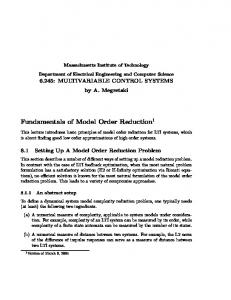
Fig. 1. The outline of the paper: conventional solution to the gear contact problems, (a) nonlinear FE method, (b) model order reduction method, and the four techniques to improve the numerical efficiency: (c) low-frequency approximation (d) ALE formulation (e) simplified dynamic equations (f) high-efficiency contact algorithm.

Another widely used MOR technique is Craig–Bampton method [14], which uses static shape vectors combined with eigenvectors obtained with fixed boundary conditions, as shown in Fig. 1(b). The main advantage of this method lies in the fulfillment of the dynamic boundary conditions and the static completeness which guarantees the same level of accuracy in static conditions for the reduced order model as the original FE model. Therefore, it was widely used in the contact problems such as the gear contact simulation [15]. However, the addition of static shape vectors for each possibly-loaded boundary DOF will result in a high-dimensional reduced order model, jeopardizing the numerical efficiency of this method. To overcome this problem, Heirman et al. [16] proposed a static mode switching (SMS) method, which was applied to the gear contact problem by Tamarozzi et al. [17]. This method uses a discontinuously changing basis matrix, which contains the static shape vectors corresponding to the actually loaded DOF, at each time-step of the simulation. When the static modes are removed or added from the mode set during simulation, the generalized coordinates of the system stay at a minimum level all the time. As a result, this approach is computationally efficient as compared with the ones where all the static modes are included. To obtain convincing results using this approach, time-integration schemes with high-frequency numerical damping have to be adopted to alleviate the discontinuities resulting from the continuous removal or addition of static shape vectors from the basis matrix [18].


71

Although the SMS approach has greatly reduced the number of DOF compared with the original FE model, the efficiency is still influenced by the resolution of the FE mesh. A parametric model order reduction (PMOR) method is introduced to solve this problem. It was first used to capture the stress fields resulting from point loads moving across the flank of the gear [19], in which the location of the contact force is parameterized. In Ref. [20], PMOR method was applied to gear contact simulations, where the flexibility of the gear is represented by a truncated set of eigenvectors and a parameter-dependent set of static shape vectors. The latter are obtained by interpolating among a set of global contact shapes, based on the rotation angles of the gear through static analysis. Due to the choice of these static shape vectors, the number of the DOF does not depend on the mesh resolution of the original FE model. Therefore, this method is insensitive to the mesh refinement and computationally efficient. However, the choice of static shape vectors may bring a series of problems [20]. As an example, the extension to a misaligned gear pair is not easy as the number of parameters describing the configuration of the gear increases from one to six and it is difficult to interpolate between six parameters. This paper tries to develop a modeling technique based on the Arbitrary Lagrangian Eulerian (ALE) formulation to reduce DOF while preserving an accurate description of gear contact problems. As the name suggests, ALE formulation is an arbitrary combination of the Lagrangian and Eulerian formulations, the advantages of which are combined together while the disadvantages are minimized [21]. The word arbitrary here refers to the fact that the combination is arbitrary which is specified by the user through the selection of mesh motion. The ALE formulation had been employed in three-dimensional beam problems to simulate a sliding joint [22] and to model axial mass flow [23]. Furthermore, it is extended to model the plates [24–26] and ropes [27,28]. In ALE formulation, the material and the mesh are not tied to each other, which provides the flexibility to choose the mesh freely. For example, a non-rolling mesh [29,30] is chosen to simulate the interaction between the rolling tire and ground, in which the contact nodes are a fixed set while the materials are flowing through the mesh nodes. A space-fixed mesh is adopted in the analysis of a belt drive [31] and reeving system [32] to avoid the moving contact between the belt/rope and pulley/sheave. The ALE formulation provides a new approach to overcome the efficiency problem in the moving load problem, where there are a large number of possibly-loaded nodes but only a few of them are loaded simultaneously. For example, when a beam moves through a curved tube, under the framework of ALE formulation, only the beam in the high-curvature section needs to be finely meshed to maintain the accuracy while coarse mesh is used in the low-curvature section to increase the computational efficiency [33]. In this paper, the Craig–Bampton method is adopted as the MOR technique and the computational efficiency of the gear contact simulation is improved through four techniques, as shown in Fig. 1(c), (d), (e), (f) respectively. First, based on the fact that the excitation frequency of gear meshing forces is much lower than the natural frequency of the gear, thereby resulting in a quasi-static response of the gear, a low-frequency approximation is adopted in the gear model by ignoring the contribution of fixed boundary normal modes and just considering the constraint modes. Second, based on the ALE formulation, only the mesh nodes of the four engaging tooth-faces are defined as boundary nodes, resulting in a great reduction in DOF of the system. Then, dynamic equations of the flexible gear are simplified by ignoring the inertial force associated with deformation, and the calculation of Jacobian matrix is also simplified. Finally, a four-step high-efficiency contact algorithm is proposed to reduce the number of contact pairs and accelerate the detection process. The first two techniques are aimed at reducing the DOF of the system. The third one concentrates on the simplification of dynamic equations and the fourth one is used to improve the efficiency of contact detection. The remainder of this paper is organized as follows. From Section 2 to Section 5, four techniques to improve the computational efficiency of a gear system are presented respectively. In Section 6, the efficiency and accuracy of the proposed method are investigated by simulating a dynamic gear contact problem and comparing results against commercial nonlinear finite element software. Finally, Section 7 summarizes the main conclusions drawn from this work. 2. The frequency analysis and low-frequency approximation of the gear To analyze the dynamic characteristics of the spur gear, a frequency analysis can be carried out using the commercial software ABAQUS [34]. The detailed process is shown in Appendix A. For a multibody system consisting of a pair of gears and shafts, as shown in Fig. 2(a), the motion of the gear and shaft is composed of the large rotation of reference frame and the accompanying elastic vibrational deformation. The excitation forces arise from the meshing forces between the gear and pinion. The excitation frequency of meshing force can be defined as meshing frequency, which is the product of the number of teeth and angular velocity of the gear, ωmesh = z gear ωgear = z pinion ωpinion . In this system, there exist significant differences of the stiffness between different components. For example, the contact

72


Fig. 2. (a) Stiffness of different components in the multibody system of shafts and gears (b) the plot of normalized amplitude (magnification factor) of gear versus frequency ratio.

stiffness between the meshing gear pairs k1 is much larger than the mesh stiffness of a single gear k2 , which is also larger than the torsional stiffness of the shaft k3 , i.e., k1 ≫ k2 > k3 . Due to its low stiffness, the natural frequency of the shaft is lower than that of the gear, see Appendix A, but higher than that of the gear–shaft pair system. To avoid the resonance of the system, the rotation speed of the gear is usually set to the sub-critical range in the design process, for example, ωgear z gear < ω4(1) /2, i.e., the excitation frequency does not exceed the half of the first-order frequency of model 4 in Appendix A. Therefore, the vibration is mainly located in the shaft and the deformation response of the gear can be approximately regarded as quasi-static (magnification factor ≈ 1) as illustrated in Fig. 2(b), which means it transmits the force from one gear to the other with time-variant static deformation. For the physical parameters of this gear, the upper limit of rotation speed can be as high as 5000 revs/min which is obtained through ωgear < ω4(1) /2z gear , considering that the natural frequency in the rotational situation is usually higher than that in the static situation. In present research, the Craig–Bampton method is used to describe the component modes of the gear. The system DOF is partitioned into boundary DOF (or interface DOF), u B , and interior DOF, u I . Two sets of mode shapes are employed in this method. One set is the constraint modes, ΦC , i.e., static shapes obtained by giving each boundary DOF a unit displacement while holding all other boundary DOF fixed. The other set is the fixed-boundary normal modes, Φ N . The relationship between the physical DOF and modal coordinates can be written as [ ] [ ] [ ][ ] [ ] qC uB I 0 qC u= = ΦC Φ N = (1) uI qN ΦI C ΦI N qN where Φ I C and Φ I N are the physical displacements of the interior DOF in the constraint modes and normal modes respectively, and qC and q N are the modal coordinates of the constraint modes and fixed-boundary normal modes. To reduce the number of DOF of the gear meshing system, the contribution of fixed boundary normal modes can be ignored where the low-frequency approximation is applicable. The number of DOF of the system is reduced from n i + zn b to zn b , where n i , zn b are the number of DOF for fixed-boundary normal modes and constraint modes respectively, z is the number of teeth and n b is the number of boundary DOF of one tooth. The relationship between the physical DOF and modal coordinates can be expressed as [ ] [ ] u qC u = B ≈ ΦC qC = (2) uI Φ I C qC 3. Model order reduction based on ALE formulation 3.1. Reduced order model of ALE gear For meshing gears, all the FE nodes of the gear on the flanks of all teeth are possibly in contact during a full revolution. For this reason, all the flanks have to be finely meshed to capture the stress field involving steep gradients. Due to the number of teeth and the mesh density required, there is a multitude of boundary nodes of the gear, which have to be reserved in the reduced-order model of the gear. In this section, a gear model based on ALE formulation is proposed to reduce the number of boundary DOF.


73

For conventional Lagrangian formulation, the mesh nodes are tied to the material points. Thus, each flank node has to be defined as a boundary node for possible contact although they are not loaded simultaneously. However, for ALE formulation, the mesh nodes can be opted not to associate with any specific material points so they are free to move through the mesh. Therefore, only the mesh nodes in “potential contact area” are defined as boundary nodes and they are invariant during the whole process, thereby achieving a great reduction in DOF of the system. The foundation of this method is based on the transmission characteristic of spur gear, i.e., either one or two pairs of teeth are in contact simultaneously. As an example, in Fig. 3, the gear is driven by the pinion and the contact ratio of this gear pair is 1.6458. The normalized time is introduced as t¯ = ∆θ/(2π/z) to describe the period from meshing-in to meshing-out for a new tooth pair, such as tooth 1 of I-gear (short for 1I) and tooth 1 of J-gear (short for 1J), where I and J refer to the pinion and gear respectively for simplicity and ∆θ is the rotation angle of 1I or 1J. The steps are as follows: (i) (ii) (iii) (iv) (v) (vi) (vii)

t¯ = 0 (Fig. 3(a)), a pair of new teeth (1I,1J) meshes in. 0 < t¯ < 0.6458, there are two pairs of teeth in mesh: (2I,2J), (1I,1J). t¯ = 0.6458 (Fig. 3(b)), the previous teeth pair (2I, 2J) meshes out. 0.6458 < t¯ < 1, there is only one pair of teeth in mesh: (1I, 1J). t¯ = 1 (Fig. 3(d)), the subsequent teeth pair (20I, 30J) meshes in. 1 < t¯ < 1.6458, there are two pairs of teeth in mesh: (1I, 1J) and (20I, 30J). t¯ = 1.6458 (Fig. 3(e)), the tooth pair (1I,1J) meshes out.

Theoretically, there are only one or two pairs of teeth in mesh simultaneously. In practice, given the backlash and the deformation of gear, the potential contact tooth-face pairs are two or four. For example, in Fig. 3 (c), the tooth-faces 2B, 1A of I-gear have possible contact with the tooth-faces 1A, 1B of J-gear (A represents the anterior face of a tooth while B refers to the posterior one). Fig. 3(a) shows that the tooth-faces 3B, 2A, 2B, 1A of I-gear and the tooth-faces 2A,2B,1A,1B of J-gear possibly have contact. To account for this in the meshing process, four tooth-face pairs are defined as the “potential contact area” in ALE formulation. For conventional Lagrangian formulation, the rotation of the gear is continuous with the teeth pair meshing-in and meshing-out one by one. In contrast, for the ALE formulation, the rotation of the gear can be decomposed into the motion of the “potential contact area” and the moving in or out process of the material points. In most of the ALE formulations, the relative movement between mesh nodes and material points is continuous [21], i.e., the material points continuously move through the mesh nodes, such as the ALE beams [23,22,33], cables [22,27], and plates [24,25]. In contrast, the prescribed relative movement in present research is a discrete one in accordance with the sequence of gear engagements, in which the mesh nodes are tied to the corresponding material points in the “potential contact area” and they are rotating forwards together during most of the time, and only at “tooth-change” instants, the mesh nodes instantaneously rotate backwards to associate with the material points of subsequent tooth-faces. From the viewpoint of material points, old material points move out of the “potential contact area” while the new ones move in. Therefore, in ALE formulation, the mesh nodes in the “potential contact area” are invariant with time, but associate with different material points at different time intervals, which is the reason why only the mesh nodes in the “potential contact area” are chosen as boundary nodes. Under the framework of ALE formulation, the number of boundary DOF is reduced from zn b to 4n b . It is clearly shown that the number of boundary DOF is determined by the mesh density n b while it is not associated to the number of teeth z. This is beneficial for the simulation of gears with many teeth. Based on floating frame of reference formulation (FFRF), as illustrated in Fig. 3(g), the generalized coordinates of I-gear, q I , are expressed as [ ]T qTI = rTI ϕ TI uTI (3) where r I , ϕ I are the position and orientation vector of the floating reference frame. u I are the modal coordinates: [ ]T u I = uT3B uT2A uT2B uT1A [[ ] [ ] ]T = u3B,1 ... u3B,25 T ... u1A,1 ... u1A,25 T (4) which consist of the modal coordinates of four tooth-faces 3B, 2A, 2B, 1A, and ui, j is the modal coordinate of node j in tooth-face i. In fact, u I represents not only the modal coordinates but also the displacements of boundary nodes. Accordingly, it forms a one-to-one correspondence from modal coordinates to boundary DOF because of the adoption of constraint modes. The displacement field of the gear can be obtained through modal transformation, see Eq. (2).

74


Fig. 3. The detailed process of gear meshing for teeth pair (1I, 1J): (a) the moment teeth pair (1I, 1J) meshes in, (b) the moment teeth pair (2I, 2J) meshes out, (c) the tooth-change moment, (d) the moment teeth pair (20I, 30J) meshes in, (e) the moment teeth pair (1I, 1J) meshes out, (f) the time period from meshing-in to meshing-out for (1I, 1J), (g) the generalized coordinates of ALE gear.

3.2. Tooth-change Accompanied with the model order reduction through ALE formulation, an important issue called “tooth-change” arises, which refers to the instantaneous process of mesh nodes rotating backwards to associate with the material points of next tooth. There are two issues concerning the “tooth-change” process: when and how. This subsection is aimed at “when” to change tooth.


75

The detailed process of tooth-change is illustrated in Fig. 3(a), (b), (c), (d), (e). At first, it is shown in Fig. 3(a) that with 1I and 1J meshing in, the number of contact tooth-face pairs changes from two (3B-2A, 2A-2B) to four (3B-2A, 2A-2B, 2B-1A, 1A-1B). Notice that the index on the left and right side of the dash refers to the tooth-face of I-gear and J-gear respectively. With the rotation moving on, the first critical moment emerges, representing the meshing-out of previous tooth pair, 2I and 2J, as shown in Fig. 3(b). The actual number of contact tooth-face pairs reduces from four (3B-2A, 2A-2B, 2B-1A, 1A-1B) to two (2B-1A, 1A-1B). With the rotation proceeding, the second critical moment emerges, as shown in Fig. 3(d), representing the meshing-in of subsequent tooth pair, 20I and 30J. The number of contact tooth-face pairs increases from two (2B-1A, 1A-1B) to four (2B-1A, 1A-1B, 1B-30A, 20A-30B) again. In the end, the meshing-out process of 1I and 1J is shown in Fig. 3(e). The number of contact tooth-face pairs reduces from four (2B-1A, 1A-1B, 1B-30A, 20A-30B) to two (1B-30A, 20A-30B). Tooth-change has to be implemented between the two critical moments, i.e., from the moment when 2I and 2J mesh out (Fig. 3(b)) to the moment at which 20I and 30J mesh in (Fig. 3(d)), during which there is only one teeth pair (two tooth-face pairs) in contact. It can be noted that there are always four tooth-face pairs defined in the simulation but for some time, there are only two tooth-face pairs actually in contact. When there are only two tooth-face pairs (2B-1A, 1A-1B) in contact, it is possible to change the previous tooth-face pairs (3B-2A, 2A-2B) not in contact to the subsequent tooth-face pairs (1B-30A, 20A-30B) which are also not in contact. The realistic tooth-change moments are t¯ = 0.6458 and t¯ = 1 while the tooth-change moment in simulation is 0.6458 < t¯ < 1. From the viewpoint of dynamics, the generalized contact forces corresponding to the boundary DOF of the previous (3B-2A, 2A-2B) and subsequent (1B-30A, 20A-30B) tooth-face pair are both zero. Fig. 4(d) shows the change of generalized contact forces before and after the tooth-change. By following this procedure, the tooth-change process can be finished smoothly. 3.3. Detailed tooth-change process This subsection is concerned about “how” to change the tooth. In general, at the “tooth-change” instants, it is a necessity to update the contact tooth-face pairs, general coordinates/velocity, modal basis matrix, stiffness matrix, and the mass matrix (nine mass invariants), which is actually the computational price of ALE formulation. 1. Change in contact tooth-face pairs To capture the contacts between an impacting gear pair correctly, the current contact tooth-face pairs have to be change to the subsequent ones during the tooth-change process. As illustrated in Fig. 4(a), the contact tooth-face pairs are changed from (3B-2A, 2A-2B, 2B-1A, 1A-1B) to (2B-1A, 1A-1B, 1B-30A, 20A-30B), see Section 5.1. 2. General coordinates/velocity transformation As shown in Fig. 4(b), the translational and rotational DOF of flexible body are kept the same after the tooth-change while the elastic deformation DOF is converted to those of the subsequent corresponding boundary DOF. This means that u3B → u2B , u2A → u1A , u2B → u1B , u1A → u20A for I-gear and u2A → u1A , u2B → u1B , u1A → u30A , u1B → u30B for J-gear. The elastic deformations of next tooth can be obtained through Eq. (2) and generalized velocity can be obtained in the same way. 3. Modal basis matrix transformation In the tooth-change process, the modal basis matrix is transformed from Φ to Φa , then Φa to Φb in two steps, where [Φ, Φa , Φb represent the mode ] matrix before transformation, after the first and second step respectively. Φ = Φ1 Φ2 ... Φi ... Φ4n b , where Φi represents the ith mode, 4n b is the number of boundary DOF of four tooth-face pairs. The detailed transformation process is shown as follows, Step 1: Each nodal displacement in the column of mode matrix has to be transferred to the corresponding one in the previous tooth because modal basis matrix is not tied to any material point in ALE formulation. Φa = TΦ where T is the transfer matrix ⎡ 0 I3n t 0 ⎢ 0 0 I 3n t ⎢ ⎢ .. .. Tz×z = ⎢ ... . . ⎢ ⎣ 0 0 0 I3n t 0 0

(5) ··· ··· .. . ··· ···

0 0 .. .

⎤

⎥ ⎥ ⎥ ⎥ ⎥ I3n t ⎦ 0

(6)

76


(a) Change in contact tooth-face pairs.

(b) General coordinates transformation (I-gear).

(c) Modal basis matrix transformation (I-gear).

(d) Change of the generalized contact force (Igear). Fig. 4. The detailed process of tooth-change: (a) contact tooth-face pairs change, (b) general coordinates transformation of I-gear, (c) modal basis matrix transformation of I-gear, (d) change of generalized contact forces of I-gear. Notice that B and A represent before and after tooth-change respectively.

( ) and I3n t = diag I3×3 ... I3×3 have n t ×n t sub-matrices, n t is the number of nodes for a single tooth. For example, in Fig. 4(c), considering the first mode, the nodal displacement vector of tooth 1 is transferred to that of tooth 20. Step 2: Due to the relative rotation δθ = 2π/z between the floating reference frame O − x y and the boundary DOF (Fig. 4(a)), coordinate transformation is made Φb = ATzn t Φa A4n b

(7)


( ) ( where A4n b = diag A ... A and ATzn t = diag AT ⎡ ⎤ cos (δθ) sin (δθ) 0 A = ⎣− sin (δθ ) cos (δθ) 0⎦ 0 0 1

...

77

) AT have 4n b × 4n b and zn t × zn t sub-matrices with (8)

4n b and zn t are the number of nodes for four contact tooth-faces and the whole gear. 4. Stiffness matrix transformation The stiffness matrix before and after the tooth-change process is essentially the same except that the set of boundary nodes is changed to the corresponding ones of the subsequent tooth. Thus, the original stiffness matrix K and the stiffness matrix after tooth-change, Ka , satisfy Ka = AT4n b KA4n b

(9)

5. Mass matrix transformation The mass matrix of a flexible body is the function of rotation parameter ϕ and elastic deformation u associated with nine constant mass parameters Ui (i = 0 ∼ 8), i.e., M = M (ϕ, u), see Eqs. (17)–(23) in Section 4. In the simplified FFRF flexible body model used in this paper, only U0 , U1 , U2 , U3 , U6 , U7 are preserved (see Eqs. (29)–(37)) and need to be updated in the tooth-change process because of the(mode matrix transformation. ) ( ) ∑ ∑ Mass invariants U0 , U1 and U6 represent the mass U0 = np=1 m p , center of mass U1 = np=1 m p s p and ( ) ∑ moment of inertia U6 = np=1 m p s˜Tp s˜ p of flexible body in floating reference frame respectively, which are not influenced by the tooth-change process. ∑ The other three mass invariants U2 , U3 and U7 have to be updated after tooth-change. U2 = np=1 m p ϕ p is taken as an example here to show the process of transformation. Due to the rotational symmetry of the gear, U2 will not be influenced by the rearrangement of node displacement vector in mode matrix (Step 1 of mode matrix transformation), i.e., Ua2 = U2 . However, since the ith modal vector of node P has to be converted from ϕ ap,i to ϕ bp,i (ϕ bp,i = AT ϕ ap,i A in Step 2 of mode matrix transformation, see Eq. (7)), the mass invariant Ub2 after tooth-change can be expressed as Ub2 =

n ∑

[ m p ϕ bp,1

...

n ] ∑ [ ϕ bp,4n b = m p AT ϕ ap,1 A

p=1

... AT ϕ ap,4n b A

]

p=1

⎛ n ∑ [ m p ϕ ap,1 = AT ⎝

...

⎞ ] ϕ ap,4n b ⎠ A4n b = AT U2 A4n b

(10)

p=1

And U3 and U7 can be updated in the same manner as U2 . The DOF associated with a gear can be reduced greatly from n i + zn b to zn b by ignoring the contribution of fixed-boundary normal modes, and from zn b to 4n b by using ALE formulation. 4. Simplified flexible body model based on floating frame of reference formulation With the low-frequency approximation, the dynamic equations of a gear can be simplified by ignoring the inertial ˙ u), ¨ which ˙ ϕ, ¨ u, u, force associated with deformation. The original generalized inertial force Qiner = Qiner (˙r, r¨ , ϕ, ϕ, is a function of translational velocity and acceleration r˙ , r¨ , and the generalized rotational coordinate, velocity, ˙ u¨ can be simplified to Qiner = ˙ ϕ, ¨ and elastic deformation and its velocity, acceleration u, u, acceleration ϕ, ϕ, ˙ ϕ), ¨ reducing the computational costs of the inertial force and Jacobian matrix. Qiner (˙r, r¨ , ϕ, ϕ, [ T ]T T As shown in Fig. 5, the generalized coordinates of a flexible body are uT , where r, ϕ [ denoted as] q = r ϕ are the position and orientation of the floating reference frame, u = u 1 ... u m is the elastic (modal) coordinate vector, and m is the number of component modes. The global position of an arbitrary point P is ( ) ( ) rp = r + A sp + up = r + A sp + ϕ pu (11) where A = A (ϕ) is the orthogonal rotation matrix A (ϕ) = I +

1 − cos ϕ sin ϕ ˜ ˜ ϕ+ ϕ˜ ϕ ϕ ϕ2

(12)

78


Fig. 5. Kinematic description used in floating frame of reference formulation (FFRF).

ϕ and ˜ ϕ are the norm and skew matrix of rotation vector ϕ ⎡ ⎤ 0 −ϕ3 ϕ2 0 −ϕ1 ⎦ ˜ ϕ = ⎣ ϕ3 −ϕ2 ϕ1 0

(13)

In the definition of the global position, s p is the position vector in the undeformed configuration and u p represents the displacement vector in[ the floating reference frame which can be obtained through mode superposition, u p = ] ∑m ϕ p u = i=1 ϕ pi u i , ϕ p = ϕ p1 ... ϕ pm is the modal basis matrix of point P. The global velocity vector of arbitrary point P is ( ) r˙ p = r˙ + Aω˜¯ s p + ϕ p u + Aϕ p u˙ (14) ¯ The angular velocity vector where ω˜¯ is the skew matrix of the angular velocity vector in the floating reference frame, ω. ˙ where H is the transformation and time derivative of generalized rotation coordinates can be related as ω¯ = HT ϕ, matrix [35] ϕ − sin ϕ 1 − cos ϕ ˜ ˜ ϕ+ ϕ˜ ϕ (15) H (ϕ) = I + ϕ2 ϕ3 The kinematic energy of the flexible body is given by Ek =

n ∑ 1 p=1

2

m p r˙ Tp r˙ p =

1 ˙ q˙ qM 2

(16)

[ ]T where q˙ = r˙ T ϕ˙ T u˙ T is the generalized velocity, n is the number of nodes, and M is the mass matrix which can be expressed in the following compact form ⎡ ⎤ Mtt Mtr Mt f Mrr Mr f ⎦ M=⎣ (17) sym Mff with Mαβ for α, β = t, r, f denotes the blocks of the mass matrix partitioned according to the system coordinates for t associated with translational coordinates, r with rotational coordinates and f with elastic coordinates, which are defined as Mtt = U0 I3×3

(18) (

˜1 + Mtr = −AU12 HT = −A U

m ∑

) ˜ 2i HT ui U

(19)

i=1

Mt f = AU2

(20)

79

J.-P. Liu et al. / Comput. Methods Appl. Mech. Engrg. 338 (2018) 68–96 Table 1 Definition of nine mass invariants. Invariant ∑ U0 = np=1 m p ∑ U3 = np=1 m p s˜ p ϕ p ∑ U6 = np=1 m p s˜Tp s˜ p

Size

Invariant ∑ U1 = np=1 m p s p ∑ U4i = np=1 m p ϕ˜ pi ϕ p ∑ U7i = np=1 m p s˜Tp ϕ˜ pi

1×1 3×m 3×3

( Mr f = HU34 = H U3 +

m ∑

Size

Invariant ∑ U2 = np=1 m p ϕ p ∑ U5 = np=1 m p ϕ Tp ϕ p ∑ U8i j = np=1 m p ϕ˜ Tpi ϕ˜ pj

3×1 3×m 3×3

Size 3×m m×m 3×3

) u i U4i

(21)

i=1

M f f = U5

(22) ⎡

Mrr = HU678 HT = H ⎣U6 +

m ∑

⎤

m ∑ m ( ) ∑ u i UT7i + U7i + u i u j U8i j ⎦ HT

i=1

(23)

i=1 j=1

where Ui (i = 0 ∼ 8) are the mass invariants, as shown in Table 1. The original form of equations of motion based on FFRF flexible body is ⎧ { [ ] } ( )T ⎪ ˙ T ˙ 1 ∂ (Mq) ∂C ∂ (Mq) ⎨ − q˙ + Kq + fe + λ=0 Mq¨ + ∂q 2 ∂q ∂q ⎪ ⎩ ˙ t) = 0 C (q, q,

(24)

where K is the stiffness matrix, fe is the generalized external forces including the contact forces between impacting ˙ t) are the constraint equations such as the joint connecting the gear to the gears and other applied forces, C (q, q, ground, and (∂C/∂q)T λ are the contribution of constraint forces. The elastic deformation of a flexible body yields elastic forces, influences the mass distribution and consequently corresponding terms in inertial forces. This simplified formulation is based on the small deformation assumption of a ˙ u¨ are assumed to be small. In addition to that, the response of the gear is flexible body and the terms concerning u, u, quasi-static and the inertial deformational forces are ignored. 4.1. Simplification of generalized inertial force In this section, the simplification of generalized inertial forces are explained in detail. 4.1.1. Simplification of acceleration term The generalized inertial forces linearly proportional to accelerations can be written as ⎡ ⎤⎡ ⎤ ⎡ ⎤ Mtt Mtr Mt f Mtt r¨ + Mtr ϕ¨ + Mt f u¨ r¨ M (q) q¨ = ⎣ MTtr Mrr Mr f ⎦ ⎣ϕ¨ ⎦ = ⎣ MTtr r¨ + Mrr ϕ¨ + Mr f u¨ ⎦ u¨ MTt f MrTf M f f MTt f r¨ + MrTf ϕ¨ + M f f u¨ ¨ Eq. (25) can be simplified to without simplification. By ignoring the contribution of u, ⎤ ⎡ ⎤ ⎡ Mtt r¨ + Mtr ϕ¨ Mtt r¨ + Mtr ϕ¨ ⎢ T ⎥ T ⎣ ⎦ M (q) q¨ ≈ Mtr r¨ + Mrr ϕ¨ ≈ ⎣ Mtr r¨ + Mrr ϕ¨ ⎦ T MTt f r¨ + MrTf ϕ¨ MTt f r¨ + Mr f ϕ¨

(25)

(26)

This can be further simplified by ignoring the deformation terms in the mass matrix. Therefore, the mass matrix will be reduced to a function of rotation vector, M = M (ϕ) as follows ˜ 1 HT ≡ Mtr Mtr = −AU12 HT ≈ −AU

(27)

Mr f = HU34 ≈ HU3 ≡ Mr f

(28)

Mrr = HU678 HT ≈ HU6 HT ≡ Mrr

(29)

80


4.1.2. Simplification of quadratic velocity term The quadratic velocity vector Qq is quadratically proportional to generalized velocities and can be expressed as { [ ] } ) ( ˙ T ˙ 1 ∂ (Mq) 1 ∂ (Mq) ˙ = Qq (q, q) − q˙ = V − VT q˙ ∂q 2 ∂q 2 ⎡ ⎤ V1 ϕ˙ + V4 u˙ )⎥ 1( T ⎢ ⎢V ϕ˙ + V5 u˙ − V1 r˙ + V2T ϕ˙ + V3T u˙ ⎥ =⎢ 2 (30) ⎥ 2 ⎣ ⎦ ) 1( T V3 ϕ˙ + V6 u˙ − V r˙ + V5T ϕ˙ + V6T u˙ 2 4 where ⎡ ⎤ 0 V 1 V4 ˙ ∂ (Mq) V= = ⎣0 V2 V5 ⎦ (31) ∂q 0 V 3 V6 ˙ Eq. (30) can be simplified by ignoring the effect of u: ⎤ ⎡ V1 ϕ˙ )⎥ 1( T ⎢ ⎢V ϕ˙ + V1 r˙ + V2T ϕ˙ ⎥ Qq ≈ ⎢ 2 ⎥ 2 ⎦ ⎣ ) 1( T V3 ϕ˙ + V4 r˙ + V5T ϕ˙ 2 Furthermore, Vi (i = 1, 2, 3, 4, 5) can be simplified as ( ) ) ( ∂ Mtt r˙ + Mtr ϕ˙ + Mt f u˙ ∂ AU12 HT ϕ˙ ˙ ∂ (AU2 u) V1 = =− + ∂ϕ ∂ϕ ∂ϕ ( ) T ˜ ∂ AU1 H ϕ˙ ≈− ∂ϕ ( ) ( ( ) ) ∂ MTtr r˙ + Mrr ϕ˙ + Mr f u˙ ∂ HU12 AT r˙ ∂ HU678 HT ϕ˙ ˙ ∂ (HU34 u) V2 = = + + ∂ϕ ∂ϕ ∂ϕ ∂ϕ ( ) ( ) T ˜ ∂ HU1 A r˙ ∂ HU6 HT ϕ˙ ≈ + ∂ϕ ) ( ∂ϕ ( T ) ( T ) T T ∂ Mt f r˙ + Mr f ϕ˙ + M f f u˙ ˙ ˙ T∂ A r T ∂ H ϕ = U2 + U34 V3 = ∂ϕ ∂ϕ ∂ϕ ( T ) ( T ) ˙ ˙ ∂ A r ∂ H ϕ ≈ UT2 + UT3 ∂ϕ ∂ϕ ) ( ( ) ∂ Mtt r˙ + Mtr ϕ˙ + Mt f u˙ ∂ AU12 HT ϕ˙ ˙ ∂ (AU2 u) V4 = =− + ∂u ∂u ∂u [ ] ˜ 21 ... U ˜ 2m HT ϕ˙ = −A U ( ) ( ) ( ) ∂ MTtr r˙ + Mrr ϕ˙ + Mr f u˙ ∂ HU12 AT r˙ ∂ HU678 HT ϕ˙ ˙ ∂ (HU34 u) V5 = = + + ∂u ∂u ∂u ∂u [ ] [ T ] T ˜ 21 ... U ˜ 2m AT r˙ + H U71 ≈H U + U71 ... U7m + U7m HT ϕ˙

(32)

(33)

(34)

(35)

(36)

(37)

4.2. Simplification of Jacobian matrix The Jacobian matrix J of FFRF flexible body takes the following form J=

∂Q ∂Q ∂Q +α + α2 ∂q ∂ q˙ ∂ q¨

(38)


(a) Coarse collision detection.

(c) Point-to-surface contact force calculation.

81

(b) Surface-to-surface contact detection.

(d) Tooth-change process.

Fig. 6. The four-step high-efficiency contact algorithm for impacting gear pairs: (a) coarse collision detection, (b) surface-to-surface contact detection, (c) node-to-surface contact force calculation, (d) tooth-change process.

where α = 1/∆t, ∆t is integration time-step, and Q is the sum of generalized inertial force Qiner and generalized elastic force Qelas , Q = Qiner + Qelas . Thus, J = Jiner + Jelas

(39)

The Jacobian matrix of generalized elastic force is constant, Jelas = K = diag(0, 0, K f f ). ˙ u) ¨ is simplified to Qiner = Qiner (˙r, r¨ , ϕ, ϕ, ˙ ϕ, ¨ u, u, ˙ ϕ), ¨ the corresponding Jacobian Since Qiner = Qiner (˙r, r¨ , ϕ, ϕ, matrix is ∂Qiner ∂Qiner ∂Qiner +α + α2 Jiner = ∂q ∂ q˙ ∂ q¨ [ ] ∂Qiner ∂Qiner ∂Qiner ∂Qiner 2 ∂Qiner +α +α + α2 0 = α (40) ∂ r˙ ∂ r¨ ∂ϕ ∂ ϕ˙ ∂ ϕ¨ In the present simulation, Jiner can be obtained through numerical difference of the Qiner , thereby reducing the number of operations required to calculate generalized inertial forces Qiner , from m + 7 to 7. 5. High-efficiency contact algorithm for gear meshing In standard contact analysis of a gear pair, all the flank nodes and elements of one gear may have contact with those of the other gear during continuous rotation. For a gear pair with z 1 and z 2 number of teeth, the maximum number of tooth-face pairs possibly in contact is n c,max = 2z 1 z 2 . Obviously, it is computationally inefficient to loop over all these tooth-face pairs and calculate the global positions of all the boundary nodes through modal transformation. This is particularly true when considering that only a small number of pairs of tooth-faces (2 or 4, depending on the single/double teeth in contact) may come into contact simultaneously. To improve the efficiency of contact detection, a four-step contact algorithm as depicted in Fig. 6(a), (b), (c), (d) is proposed in this paper. The algorithm is as follows:

82


Step 1: coarse collision detection. It is used to identify the four tooth-face pairs possibly in contact. Step 2: surface-to-surface contact detection. It is used to identify which two element-faces of a tooth-face pair are possibly in contact by looping over all the element-faces in each tooth-face. The bounding sphere method is used to accelerate the process. Step 3: node-to-surface contact force calculation. It is used to calculate the contact force between two element-faces through a penalty method. Step 4: tooth-change process. It is used to update the current four pairs of tooth-faces in contact to the subsequent ones at the right time to capture the contact between gear pairs correctly. 5.1. Coarse collision detection and tooth-change process First, a simple two-dimensional case as depicted in Fig. 7(a) is used to illustrate the coarse collision process. In this case, both gears are hinged to the ground using a revolute joint. Accordingly, the parallelism of the two gear axes is guaranteed. Two reference frames are introduced to measure the angular position of I-gear. One is the body-fixed reference O1 − x y. The other is the space-fixed reference O1 − x0 y0 , the origin of which is located in the center of I-gear, the direction of the x-axis is pointing from the center of I-gear to that of J-gear. The angular difference θ (t) between O1 − x y and O1 − x0 y0 is defined as the angular position of I-gear. As can be seen in Fig. 7(a), at the initial moment t¯ = 0, 1I and 1J mesh have four contact tooth-face pairs (3B-2A, 2A-2B, 2B-1A, 1A-1B), and the angular position of I-gear is θ0 . To identify the four pairs of tooth-faces in contact during the following revolution, the angular displacement ∆θ = θ − θ0 is introduced. With the I-gear rotating anti-clockwise, ∆θ increases and can be used to update the contact tooth-face pairs. Within the framework of ALE formulation, the tooth-change process has to be implemented during the one-tooth in contact period. For example, in this case, the contact ratio is 1.6458, thereby the tooth-change process has to be accomplished at a series of time instants t¯ci = t¯c + i, i = 1, 2, 3..., where t¯c is the tooth-change time threshold, 0.6458 < t¯c < 1. At each time moment ∆θ (t) = t¯ci · (2π/z), i = 1, 2, 3..., the contact tooth-face pairs are updated to the successive ones. In this case, when ∆θ = t¯c · (2π/z), the contact pairs are updated from (3B-2A, 2A-2B, 2B-1A, 1A-1B) to (2B-1A, 1A-1B, 1B-30A, 20A-30B) and to (1B-30A, 20A-30B, 20B-29A, 19A-29B) when ∆θ = (t¯c + 1) · (2π/z). Therefore, the key procedures in coarse collision detection are to define the contact tooth-face pairs at the initial time and obtain the angular displacement of I-gear in each time step. Then, the contact tooth-face pairs can be updated to the subsequent ones according to the tooth-change time threshold. In three-dimensional contact, the axes of two gears are not perfectly aligned because of the elastic deformation of the shaft. Therefore, a generalized approach has to be introduced to define angular position of I-gear while the other procedures are the same as those in the two-dimensional case. As illustrated in Fig. 7(b), reference frame O1 − x0 y0 z 0 is introduced to define the angular position of I-gear. The origin of O1 − x0 y0 z 0 is fixed with the center of I-gear and its x-axis is from O1 to O2 . Accordingly, the z-axis can be obtained as follows ( ) zˆ 0 = zˆ − zˆ T xˆ 0 xˆ 0 (41) where xˆ 0 , zˆ 0 are the x-axis and z-axis of O1 − x0 y0 z 0 , zˆ is z-axis of body-fixed frame O1 − x yz of I-gear. Then, the y-axis of O1 − x0 y0 z 0 is given by yˆ 0 = zˆ 0 × xˆ 0 . In O1 − x0 y0 z 0 frame, the angular position θ of I-gear is given by ( T ) ˆ yˆ 0 −1 x θ = tan (42) xˆ T xˆ 0 which measures the angular position θ in three-dimensional space, in which the x y plane may not coincide with x0 y0 plane. It should be pointed out that Eq. (42) is acceptable for small rotations, in which the angular difference α between the z-axes of O1 − x0 y0 z 0 and O1 − x yz is small, usually less than 10◦ . This is the case for gear contact simulation. 5.2. Surface-to-surface detection acceleration using bounding sphere method After four pairs of contact tooth-faces are identified, the contact forces between each pair can be obtained. For a tooth-face pair meshed with n 1 and n 2 element-faces, the number of element-face contact pairs is n 1 × n 2 by looping over each element-face of the tooth-face. It is noted that only a small part of them may have contact, since the theoretical contact area for two meshing spur gears is a line, and only the element-faces adjacent to this line have


83

Fig. 7. The coarse collision process: (a) two-dimensional case, (b) three-dimensional case.

possible contact. To avoid too many useless evaluations of element-face pairs, the bounding sphere method is adopted to accelerate the contact detection process. The core of this method is to replace the contact between two element-faces with two bounding spheres which are easy to judge whether they have contact or not and quickly eliminate the pairs that could not possibly be in contact. The whole process is divided into two steps, the details of which are shown in Refs. [36,37]. Step 1: bounding sphere construction. It is used to construct a bounding sphere for each element-face such as a triangle or quadrilateral (element-face of tetrahedron and hexahedron element). Step 2: overlap detection between spheres. It is used to identify which pair of n 1 × n 2 pairs of bounding spheres may have possible contact by comparing the distance between the sphere centers against the sum of the sphere radii. 5.3. Point-to-surface contact formulation Without loss of generality, the FE model of gear is meshed with eight-node hexahedral elements and the corresponding element-faces are quadrilaterals as illustrated in Fig. 6(c). A general point-to-surface contact scheme is adopted, which involves a slave node and a master surface. The Gauss integration points of one of the element-faces are chosen as the slave nodes with the other element-face as the master surface. The global position of an arbitrary point in the element-face can be obtained by r (ξ, η) =

4 ∑

[ Ni ri = N1 I3×3

N2 I3×3

N3 I3×3

] N4 I3×3 q = Nq

(43)

i=1 T where arbitrary point (ξ, η) in the local frame is mapped to the point [ ] r = [x, y, z] in the global frame, ri is the coordinate of the corner node Pi (i = 1 ∼ 4), q = rT1 rT2 rT3 rT4 are the generalized coordinates of the element,

84


[ N = N1 I3×3

N2 I3×3

N3 I3×3

] N4 I3×3 is the shape function, which is expressed as

1 1 (ξ − 1) (η − 1) N2 = − (ξ + 1) (η − 1) 4 4 1 1 N3 = (ξ + 1) (η + 1) N4 = − (ξ − 1) (η + 1) (44) 4 4 To obtain the projection point P of point A, the geometric conditions ∂r ∂r =0 =0 (45) [R − r (ξ, η)]T [R − r (ξ, η)]T ∂ξ ∂η are imposed. This implies that the projection vector P A must be perpendicular to the tangent vector of the surface, where R and r are the positions of points A and P, ∂r/∂ξ, ∂r/∂η are the tangent vectors of point P. These two non-linear equations can be iteratively solved using Newton–Raphson method. The penetration depth δ of point A is given by ∂r/∂ξ × ∂r/∂η δ = −(R − r)T n (46) n= ∥∂r/∂ξ × ∂r/∂η∥ where n is the unit normal vector at point P. If δ < 0, there is no interaction between point A and the surface and the contact force is zero. When δ > 0, the normal contact force is ( ) Fn = Fn n = K δ e + cδ˙ n (47) N1 =

where Fn is the value of normal contact force Fn , K is the normal stiffness, c is the normal damping ratio, e is the nonlinear exponent, and δ˙ is the normal penetration velocity of point A, which is ˙ Tn δ˙ = −(v A − v P )T n = −[v A − N (ξ P , η P ) q]

(48)

˙ where where of points A and P, v A is obtained in its element-face while v P = N (ξ P , η P ) q, [ v A , v P are the velocities ] q˙ = r˙ T1 r˙ T2 r˙ T3 r˙ T4 is the generalized velocity. Velocity-based friction model [38] is adopted to calculate the tangential friction force, Ft = µ f Fn , where µ f is the coefficient of friction ⎧ step (vt , −vs , µs , vs , −µs ) (−vs ≤ vt ≤ vs ) ⎨ µ f (vt ) = −sgn (vt ) · step (|vt | , vd , µd , vs , µs ) (vs < |vt | < vd ) (49) ⎩ −sgn (vt ) · µd (|vt | ≥ vd ) in which µd is the dynamic coefficient of friction, µs is the static one, vs is the static transition velocity, and vd is the dynamic transition one, vt is the norm of tangential slip velocity of point A with respect to point P, vt = vt τ [ ] vt vt = (50) vt = (v A − v P ) − (v A − v P )T n n τ= ∥vt ∥ vt The step function in Eq. (49) is defined as ⎧ h0 (t ≤ 0) ⎨ step (x, x0 , h 0 , x1 , h 1 ) = h 0 + (h 1 − h 0 ) (3 − 2t) t 2 (0 < t < 1) (51) ⎩ h1 (t ≥ 1) where t = (x − x0 ) / (x1 − x0 ). It is noted that the frictional force Ft is zero when vt = 0. The total contact force can be obtained through F = Fn + Ft , where Ft is the tangential frictional force, Ft = µ f Fn τ . F is applied at slave point A and its reaction force −F is distributed to four master nodes, P1 , P2 , P3 , P4 according to the principle of virtual work, δrT (−F) = −δqT NT F = δqT Qr ]T [ (52) Qr = FrT1 FrT2 FrT3 FrT4 = −NT F where Fri (i = 1 ∼ 4) is the reaction force applied at node Pi , Fri = −Ni F. The choice of which of the two flexible bodies is the master body and which one is the slave one might slightly affect the results [17]. In this study, a general two-pass algorithm in Ref. [17] is adopted in which the two flexible gears are alternatively chosen as master or slave body and the contact force is the weighted average result with a weight factor w f ∈ [0, 1]. In this approach, w f = 0, 1 represents the situation where one of the gears is chosen as the master body, the other as slave body, and no average is used.


85

Fig. 8. The FE model used in the numerical simulation. Table 2 Basic parameters of gear and pinion. Parameters

Pinion

Gear

Number of teeth Pressure angle (◦ ) Normal module (mm) Face width (mm) Base circle radius (mm) Pitch circle radius (mm) Addendum circle radius (mm) Dedendum circle radius (mm) Nodes per flank Number of nodes Number of elements

13 20 8 40 48.864 52 60 42 121(11 × 11) 33605 27820

97 20 8 40 364.6005 388 396 378 66(11 × 6) 60528 43650

6. Numerical examples Four numerical examples are given in this section to verify the proposed method. The FE models of the pinion and gear used in the numerical simulation are shown in Fig. 8 and the basic parameters are provided in Table 2. Both of the gears are meshed by the hexahedral elements, and fine meshes are used in the potential contact area of tooth flanks. All the nodes on the bore surface are rigidly connected to the center of the gear (MPC element), where the origin of floating frame of reference is based. In the simulation, a material with Young’s modulus E = 210 GPa, density ρ = 7860 kg/m3 and Poisson’s ratio ν = 0.3 is used. 6.1. Static completeness verification This example is used to verify the static completeness of the proposed ALE formulation. In the example, the center of the gear is fixed on the ground and static distributed load F = 6.875 × 104 N/m is applied on tooth-face 2A in −y direction, as illustrated in Fig. 9(a). This problem is solved by the nonlinear FE software ABAQUS and the in-house code based on the method introduced in this paper. In present formulation, all the nodes on tooth-face 2A are defined as boundary nodes, which are mapped to a 11 × 11 unit mesh (χ η) to compare the results more clearly. Fig. 9(b) shows three-dimensional Mises stress pattern given by ABAQUS and the location of maximum stress is at the load point on both ends. In Fig. 9(c) and (d), the vertical displacement U y and Mises stress of tooth-face 2A are compared between ABAQUS and in-house code. As can be seen from the figure, the results are in good agreement with one

86


Fig. 9. The static completeness verification: (a) schematic of a gear subjected to distributed load F, (b) three-dimensional Mises stress pattern of the gear, and comparison between ABAQUS and in-house code on tooth-face 2A: (c) vertical displacement U y , (d) Mises stress. Table 3 Comparison of the maximum deflection and Mises stress between ABAQUS and in-house code.

Maximum deflection (mm) Maximum Mises stress (MPa)

ABAQUS

In-house code

Relative error (%)

−8.54794 × 10−2

−8.547936 × 10−2

1828.8

1828.801

0.000047 0.000055

another. The comparisons of maximum deflection and Mises stress are shown in Table 3, where the relative error is less than 0.0001%. It is worth mentioning that the number of DOF is greatly reduced from 446439 of FE method to 369 through ALE formulation, while the accuracy is maintained. 6.2. Static contact verification In this example, the gear is fixed on the ground while the pinion is free to rotate around its z-axis. A torque M = 1225 Nm is then applied on the pinion and only one teeth pair is in contact. Under the framework of ALE formulation, the pinion and gear are modeled with 363(= 11 × 11 × 3) and 198(= 11 × 6 × 3) boundary modes, respectively, to obtain a statically complete result. This is important as all the nodes on a tooth flank could come into contact. The number of DOF is 573, which is the sum of flexible modes (363 + 198) and rigid DOF (6 + 6), compared with 1161741 of ABAQUS model. To guarantee the accuracy of contact detection, 4 × 4 Gauss points in a element-face are used in the simulation. Fig. 10(a) and (b) compare the Mises stress patterns of the gears’ sides given by the non-linear FE method and present ALE formulation. As can be seen, both qualitative and quantitative matching are achieved. The in-house code and ABAQUS software give the maximum Mises stress as 245.14 MPa and 247.1 MPa, respectively, resulting in a relative error of 0.79%. Fig. 10(c) and (d) show the three-dimensional Mises stress distribution of the pinion and gear, especially in the vicinity of upper tooth-root. To compare the results more clearly, the upper tooth-root areas of the pinion and gear are mapped to a 11 × 5 and 6 × 4 unit mesh (χ η) respectively.


87

Fig. 10. The static contact verification: comparison of Mises stress pattern of gears’ sides, (a) ABAQUS (b) in-house code, and comparison of Mises stress distribution near the tooth-root between ABAQUS and in-house code, (c) pinion, (d) gear. Table 4 Comparison of the reaction force and moment between ABAQUS and inhouse code.

Pinion Fx (N) Pinion Fy (N) Gear Mz (Nm)

ABAQUS

In-house code

Relative error (%)

8625.96 23644 9178.87

8574.48 23520.3 9123.94

0.6 0.52 0.6

As shown in Fig. 10(c) and (d), the results between two methods are in good agreement. Table 4 compares reaction force and moment between ABAQUS and in-house code and the difference is less than 1%. The slight discrepancy might arise from the difference in the contact algorithm because our simulation is based on node-to-surface contact while the ABAQUS uses surface–surface contact [34]. 6.3. Dynamic verification of tooth-change process In this example, both the gear and pinion are hinged to the ground with revolute joints along its z-axis. The simulation is performed by applying rotational velocity constraint to the gear (driving gear) while the pinion (driven gear) is left to rotate with a resistant torque M = 1225 × step(0, 0, 1, 1) Nm. The step function is defined in Eq. (51).

88


Fig. 11. The engagement and tooth-change process of six tooth pairs for (a) gear, and (b) pinion.

A quasi-static situation is considered in this example with angular velocity of gear ω = 0.01 × step(0, 0, 1, 1) rad/s. The simulation covers the engagement process of six pairs of teeth within 40s of physical time. Fig. 11 shows the engagement and tooth-change process of six pairs of teeth. In this figure, the x-axis is the normalized time t¯ = ∆θ (t) / (2π/z), representing the number of rotation teeth from the beginning while y-axis is the tooth index. During the meshing process, there are four contact tooth-face pairs formed from four tooth-faces from three teeth of the pinion and four tooth-faces from two teeth of the gear. In Fig. 11, it can be seen that tooth 1, 2, and 3 of the pinion (tooth-face 1A, 2B, 2A, 3B actually) mesh with tooth 1 and 2 of the gear (tooth-face 1B, 1A, 2B, 2A in fact) at the first engagement. To realize continuous rotation, tooth-change has to be carried out. In this example, the tooth-change threshold is adopted as t¯c = 0.5, which means the contact tooth-face pairs are updated to the next ones at a series of time instants t¯ = t¯c + i = 0.5 + i, i = 0, 1, 2, 3... (orange dash line in Fig. 11). The FE mesh is the same as the previous two examples while the number of DOF is close to four times the size of example 2 for ALE formulation, due to that the nodes of four tooth-faces are adopted as boundary nodes, i.e., tooth-face 1A, 2B, 2A, 3B of the pinion and tooth-face 1B, 1A, 2B, 2A of the gear. The influence of tooth-change threshold t¯c is shown in Fig. 12, in which dynamic transmission error (DTE) and Mises stress are used to assess the accuracy of the proposed method. DTE is defined as the difference between the actual position and the theoretical position that the gear would occupy if the gear teeth are considered perfect and rigid, and it is an important characteristic in the study of gear vibration and noise [39,40]. Fig. 12(a) shows DTE (θc − θt ) of pinion center where θc and θt are the actual and theoretical angular displacements of the center. In this figure, the meshing-out moments are (k +0.44), where k is a positive integer which is illustrated in blue dot–dash lines, and the meshing-in moments are (k + 0.63) represented by the orange dot–dash lines. As pointed out in Section 3, tooth-change has to be carried out during the one-tooth-in contact period, i.e. t¯ ∈ (0.44, 0.63) in this case. Therefore, four different tooth-change thresholds are chosen as: 0.4, 0.5, 0.6, 0.7 to investigate the influence. It can be seen from the figure that results for t¯c = 0.5, 0.6 are in very good agreement. However, for t¯c = 0.4, tooth-change moment is prior to the meshing-out of the previous tooth. This means that although the previous two tooth-face pairs are still in contact (there are four tooth-face pairs in total), the contact tooth-face pairs are changed to the next two which are not in contact yet. It leads to the sudden increase of the DTE ahead of its schedule (actually, we refer to the absolute value of (θc − θt ) because θc − θt < 0), which is inconsistent with the real situation. Similarly, for t¯c = 0.7, tooth-change moment is posterior to the meshing-in of the next tooth, which means although the next two tooth-face pairs are already in contact, the contact tooth-face pairs have not yet been transferred from the previous two not-in-contact pairs to the next two. It leads to the delay of the sudden drop of DTE. Fig. 12(b) shows the Mises stress of point 1 of the pinion tooth. Similar to the result of DTE, the results for t¯c = 0.5, 0.6 are almost the same while t¯c = 0.4 leads to the sudden increase of Mises stress happening ahead of its schedule and t¯c = 0.7 results in the delay of the sudden drop of Mises stress due to the inappropriate tooth-change moments. It is noted that there are no obvious oscillations in the vicinity of tooth-change moments in the presented simulation, which verifies the smoothness and effectiveness of tooth-change methods in the present ALE formulation.


89

Fig. 12. Comparison between different tooth-change thresholds of (a) pinion DTE (θc − θt ) of center (b) stress of point 7 of tooth 1 of the pinion. For clear illustration, the meshing-out (blue dot–dash line) and meshing-in (orange dot–dash line) moments for a tooth are shown in the figure.

6.4. Dynamic verification of accuracy and efficiency In this example, the accuracy and efficiency of the ALE method are compared with those of the nonlinear FE method. This model is the same as the one studied in Section 6.3, but with ω = 50 × step(0, 0, 0.1, 1) RPM and M = 1225 × step(0, 0, 0.1, 1) Nm. The simulation experiences 0.3s, covering about the engagement process of 20 pairs of teeth (about 1.5 cycles of pinion), and the acceleration process is 0.1 s. Fig. 13(a) shows the DTE of the gear. In this figure, θi is the angular displacement of point i (i = 1, 4, 7, 10) of tooth 97, θc and θt are the actual and theoretical angular displacements of the center, which are the same for the driving gear (θc = θt ). θi − θt represents the angular deflection of point i caused by elastic deformation. It is clearly shown in Fig. 13(a) that the angular deflections are almost the same for different regions of tooth 97 of the gear during the non-meshing period while increases from the root to tip (point 10→point 7→point 4→point 1) in meshing period, i.e., t¯ ∈ (0.63, 2.44) for the acceleration process. Fig. 13(b) shows the angular deflections of the pinion (tooth 1), the result of which is very similar to the gear, except that there are two peaks. The first peak is t¯ ∈ (0.63, 2.44) for acceleration process and the second peak is t¯ ∈ (13.63, 15.44) for stable process. Because the pinion is the driven gear, the contact force is in the same direction as the deflection so that θi − θc > 0 (Fig. 13(b)) while θi − θc (θt ) < 0 (Fig. 13(a)) for the driving gear. It can be noted that the angular deflection of the gear is less than that of the pinion because of its larger radius. Fig. 13(d) shows the DTE (θc − θt ) of the pinion center, which has two typical regions, high DTE region t¯ ∈ (k + 0.44, k + 0.63) for single-pair contact and low DTE region t¯ ∈ (k + 0.63, k + 1.44) for double-pair contact, where k is a positive integer. There are steep transitions between these regions, representing the meshing-out (k + 0.44, blue dot–dash line) and meshing-in moments (k + 0.63, orange dot–dash line). Fig. 13(c) is the sum of Fig. 13(b) and Fig. 13(d), i.e., (θi − θt ) = (θi − θc ) + (θc − θt ), representing the DTE of points 1, 4, 7 and 10. In Fig. 13(b), θi − θc > 0 while in Fig. 13(d), θc − θt < 0, but in Fig. 13 (c), θi − θt < 0, which shows a larger influence of rigid rotation compared with the flexible deformation. Overall, the DTE results of the ALE formulation closely agree with those of the non-linear FE method. The differences between these results can be attributed to the ignorance of higher frequency modes and the difference in contact-detection algorithm between ABAQUS and in-house code.

90


Fig. 13. Comparison of DTE between ALE formulation and nonlinear FE method, (a) DTE (θ − θc ) of points 1, 4, 7 and 10 of tooth 97 of the gear (b) DTE (θ − θc ) of points 1, 4, 7 and 10 of tooth 1 of the pinion (c) DTE (θ − θt ) of points 1, 4, 7 and 10 of tooth 1 of the pinion (d) pinion DTE (θc − θt ) of center. For clear illustration, the meshing-out (blue dot–dash line) and meshing-in (orange dot–dash line) moments for a tooth are shown in the figure. Black dash line stands for a complete cycle of the pinion.

Fig. 14(a) shows the Mises stress of the pinion, in which σ Mi is the stress of point i (i = 1, 4, 7, 10) of tooth 1. It is clearly shown that the stresses are almost zero for different regions of the pinion during the non-meshing period. There are also two peaks during the meshing period, the first of which is t¯ ∈ (0.63, 2.44) in acceleration process and the second is t¯ ∈ (13.63, 15.44) in stable process. By analyzing the second peak period as an example, the tooth-root stress of point 7 suddenly increases when it meshes in (t¯ = 13.63) or the previous tooth meshes out (t¯ = 14.44), and it drops when the subsequent tooth meshes in (t¯ = 14.63) or itself meshes out (t¯ = 15.44). This is in close agreement with ABAQUS results. For points 1 and 4 of the pinion, the stress level is lower than that of point 7 and the time history is similar. However, for point 10, it experiences two continuous peaks because it is the tooth root both for tooth 1 and the previous tooth, tooth 2. During the first half meshing process of tooth 2 (t¯ ∈ (12.63, 13.63)), point 10 is in the area of compressive stress which continuously increases. Then, the stress of point 10 drops suddenly because


91

Fig. 14. Comparison of Mises stress between ALE formulation and nonlinear FE method, (a). stress of points 1, 4, 7 and 10 of tooth 1 of the pinion (b). stress of points 1, 4, 7, and 10 of tooth 97 of the gear. For clear illustration, the meshing-out (blue dot–dash line) and meshing-in (orange dot–dash line) moments for a tooth are shown in the figure.

the tensile stress caused by meshing-in of tooth 1 counteracts the compressive stress caused by tooth 2, after which it behaves just like point 7. For points 1, 4, 7, and 10 of the gear, the situation is a little different because points 1, 4, 7, and 10 of the pinion are not in the contact tooth-face while the corresponding points of the gear are in the contact tooth-face. It can be seen from Fig. 14(b) that the stress of points 7, 4, and 1 increases from zero successively. This means that they have contact from the root (point 7) to the middle (point 4) until the tip (point 1), which correlates to the realistic situation qualitatively. For point 10, it is also located in the transition area between tooth 97 and 1. Therefore, it also has two continuous peaks just like point 10 in the pinion. Fig. 15 shows the time history of the first six teeth of the pinion and gear and it is noted that the pinion has rotated more than one circle. In the stable process of rotation, the stress curves for different teeth are the same because of the rotational symmetry of the gear. The reaction force and moment between ALE formulation and nonlinear FE method are shown in Fig. 16, which also indicates the accuracy of the ALE formulation. Finally, the computational costs of two formulations are compared. It takes about 180 h to finish this task using ABAQUS, while only 8.4 h are used to obtain comparable results with present ALE formulation. This implies that computational efficiency of the proposed method is one order of magnitude better in this typical example when compared to the conventional method. 7. Conclusions In this paper, a novel model order reduction method based on ALE formulation is developed to improve the efficiency of the gear contact simulation. The efficiency has been achieved by the following four techniques. First, a low-frequency approximation of the gear model is adopted, which is valid when the rotation speed of the gear pair is a fraction of the natural frequency of the gear. Second, by taking advantage of ALE formulation, the mesh nodes and the materials are not tied together, and only the mesh nodes of four tooth-faces are defined as boundary nodes which are associated with different material points at different times. These two techniques are designed to reduce the DOF of the gear pair, from n i + zn b to zn b by ignoring the fixed boundary normal modes, and from zn b to 4n b by using ALE formulation. The third technique focuses on the simplification of inertial force and Jacobian matrix by ignoring the

92


Fig. 15. Time evolution of the Mises stress for different teeth of (a) pinion and (b) gear. For clear illustration, the meshing-out (blue dot–dash line) and meshing-in (orange dot–dash line) moment for a tooth is shown in the figure.

Fig. 16. Comparison between ALE formulation and nonlinear FE method, (a) reaction force of pinion (b) reaction moment of pinion. For clear illustration, the meshing-out (blue dot–dash line) and meshing-in (orange dot–dash line) moment for a tooth is shown in the figure.

contributions from deformation. Finally, a four-step high-efficiency contact algorithm is used to reduce the number of contact pairs in the detection process and improve the efficiency through coarse collision detection and bounding sphere method. Four numerical examples demonstrated the accuracy and efficiency of the proposed method. Acknowledgments Supports from National Natural Science Foundation of China (11302114), Beijing Nova Program Interdisciplinary Cooperation Project (xxjc201705) and Major State Basic Research Development Program (2012CB821203) are acknowledged. The authors also thank Dr Jiang Cui, Dr Cameron Dennis and Marilyn An for their helpful discussion and revision on this paper and Jiawei He for his contribution on post-processing software.


93

Fig. A.17. (a) The FE model of a spur gear (b) four different models of gear and shaft. Table A.5 Parameters of the gear. Number of tooth Normal module Pressure angle Face width

13 6 mm 20◦ 40 mm

Base circle radius Pitch circle radius Addendum circle radius Dedendum circle radius

48.864 mm 52 mm 60 mm 42 mm

Table A.6 Natural frequencies of four different models of gear and shaft. Order

1 2 3 4 5 6

Natural frequency (Hz) Model 1

Model 2

Model 3

Model 4

5443.2 9043.4 9043.4 10491 12540 12540

2864.9 2864.9 5275.7 6577.6 6577.6 8506.9

2226.3 2226.3 3331.5 6076.2 6076.2 6737.7

2217.2 2217.2 2961.8 5716.1 5716.1 6213.2

Appendix A. Frequency analysis of the spur gear A three-dimensional FE model of a spur gear was established by using ABAQUS software [34], as shown in Fig. A.17(a). The parameters of the gear are shown in Table A.5. The length of the shaft is 300 mm with a circular cross section of 35 mm radius. In the simulation, a material with Young’s modulus E = 210 GPa, density ρ = 7860 kg/m3 and Poisson’s ratio ν = 0.3 is used. Without loss of generality, four different models are simulated, as shown in Fig. A.17(b). (i) only the flexible gear: the center of the gear is fixed on the ground (ii) only the flexible shaft: both ends of the shaft are fixed on the ground (iii) rigid gear mounted on a flexible shaft: the center of the gear is fixed on the shaft, both ends of which are fixed on the ground (iv) flexible gear mounted on a flexible shaft: the center of the gear is fixed on the shaft, both ends of which are fixed on the ground The natural frequencies and modes of different models are shown in Tables A.6 and A.7. Fig. A.18(a) shows the first six vibration modes of the flexible gear fixed on the ground. The first mode is almost circumferential without axial vibration. The second and third modes have the same natural frequency and are mainly first-order bending vibration modes. The fourth mode is mainly axial vibration and just like an umbrella. The fifth and sixth one are second-order bending vibration modes. For the other three models with flexible shafts, the vibration modes are pretty similar, thereby the model of the flexible gear mounted on the flexible shaft is chosen as a representative to show the results, as illustrated in Fig. A.18(b). The first two modes are mainly about the first-order bending vibration of the shaft and

94


Table A.7 Modes of four different models of gear and shaft. Order

Mode description Model 1

Model 2

Model 3

Model 4

1 2 3 4 5 6

Circumferential 1-order bending 1-order bending Axial 2-order bending 2-order bending

1-order bending 1-order bending Torsional 2-order bending 2-order bending Axial



Fig. A.18. (a) The first six modes of the flexible gear fixed on the ground (b) the first six modes of the flexible gear fixed on the flexible shaft.

gear. The third mode is the torsional one. The fourth and fifth modes are second-order bending modes of the shaft and gear. The sixth mode is the axial mode of the shaft and gear. For the ith mode (i = 1 ∼ 6), the relationship between the natural frequencies of models 2, 3, and 4 is ω4(i) < ω3(i) < ω2(i) because model 4 is more flexible than model 3 and model 3 has more mass than model 2. Comparing the natural frequency between model 1 and 2, we can see that the stiffness of the gear is higher than that of the shaft, which is the main source of flexibility of the gear–shaft system. Furthermore, the deformation of the gear is negligible compared with that of the shaft and is just used to transmit the


95

meshing force from one gear to the other because the difference of first-order frequencies between model 3 and 4 is very small. Appendix B. Supplementary data Supplementary material related to this article can be found online at https://doi.org/10.1016/j.cma.2018.03.039. References [1] V.K. Tamminana, A. Kahraman, S.M. Vijayakar, A study of the relationship between the dynamic factors and the dynamic transmission error of spur gear pairs, J. Mech. Des. 129 (1) (2007) 75–84. [2] M.A. Hotait, A. Kahraman, Experiments on the relationship between the dynamic transmission error and the dynamic stress factor of spur gear pairs, Mech. Mach. Theory 70 (2013) 116–128. [3] H.N. Özgüven, D.R. Houser, Mathematical models used in gear dynamics –a review, J. Sound Vib. 121 (3) (1988) 383–411. [4] Q. Tian, Q.F. Xiao, Y.L. Sun, H.Y. Hu, H. Liu, P. Flores, Coupling dynamics of a geared multibody system supported by elastohydrodynamic lubricated cylindrical joints, Multibody Syst. Dyn. 33 (3) (2015) 259–284. [5] R.G. Parker, S.M. Vijayakar, T. Imajo, Non-linear dynamic response of a spur gear pair: modelling and experimental comparisons, J. Sound Vib. 237 (3) (2000) 435–455. [6] C.G. Cooley, R.G. Parker, S.M. Vijayakar, A frequency domain finite element approach for three-dimensional gear dynamics, J. Vib. Acoust. 133 (4) (2011) 041004. [7] R.G. Parker, V. Agashe, S.M. Vijayakar, Dynamic response of a planetary gear system using a finite element/contact mechanics model, J. Mech. Des. 122 (3) (2000) 304–310. [8] A. Andersson, L. Vedmar, A dynamic model to determine vibrations in involute helical gears, J. Sound Vib. 260 (2) (2003) 195–212. [9] N. Cappellini, T. Tamarozzi, B. Blockmans, J. Fiszer, F. Cosco, W. Desmet, Semi-analytic contact technique in a non-linear parametric model order reduction method for gear simulations, Meccanica 53 (1–2) (2018) 49–75. [10] S.M. Vijayakar, A combined surface integral and finite element solution for a three-dimensional contact problem, Internat. J. Numer. Methods Engrg. 31 (3) (1991) 525–545. [11] P. Ziegler, P. Eberhard, Simulative and experimental investigation of impacts on gear wheels, Comput. Methods Appl. Mech. Engrg. 197 (51) (2008) 4653–4662. [12] P. Ziegler, P. Eberhard, B. Schweizer, Simulation of impacts in geartrains using different approaches, Arch. Appl. Mech. 76 (9) (2006) 537–548. [13] P. Ziegler, P. Eberhard, Investigation of gears using an elastic multibody model with contact, in: Multibody Dynamics, Springer, 2011, pp. 309–327. [14] R. Craig, M. Bampton, Coupling of substructures for dynamic analyses, AIAA J. 6 (7) (1968) 1313–1319. [15] G. Virlez, O. Brúls, V. Sonneville, E. Tromme, P. Duysinx, M. Géradin, Contact model between superelements in dynamic multibody systems, in: ASME 2013 International Design Engineering Technical Conferences and Computers and Information in Engineering Conference, American Society of Mechanical Engineers, 2013, pp. V07AT10A050, Portland, Oregon, USA. [16] G.H. Heirman, T. Tamarozzi, W. Desmet, Static modes switching for more efficient flexible multibody simulation, Internat. J. Numer. Methods Engrg. 87 (11) (2011) 1025–1045. [17] T. Tamarozzi, P. Ziegler, P. Eberhard, W. Desmet, Static modes switching in gear contact simulation, Mech. Mach. Theory 63 (2013) 89–106. [18] T. Tamarozzi, G.H. Heirman, W. Desmet, Static modes switching: on-line variable static augmentation for efficient flexible multibody simulation, in: ASME 2011 International Design Engineering Technical Conferences and Computers and Information in Engineering Conference, American Society of Mechanical Engineers, 2011, pp. 1087–1099. [19] T. Tamarozzi, G.H. Heirman, W. Desmet, An on-line time dependent parametric model order reduction scheme with focus on dynamic stress recovery, Comput. Methods Appl. Mech. Engrg. 268 (2014) 336–358. [20] B. Blockmans, T. Tamarozzi, F. Naets, W. Desmet, A nonlinear parametric model reduction method for efficient gear contact simulations, Internat. J. Numer. Methods Engrg. 102 (5) (2015) 1162–1191. [21] T. Belytschko, W.K. Liu, B. Moran, K. Elkhodary, Nonlinear Finite Elements for Continua and Structures, John Wiley & Sons, 2013. [22] D.F. Hong, G.X. Ren, A modeling of sliding joint on one-dimensional flexible medium, Multibody Syst. Dyn. 26 (1) (2011) 91–106. [23] D.F. Hong, J.L. Tang, G.X. Ren, Dynamic modeling of mass-flowing linear medium with large amplitude displacement and rotation, J. Fluids Struct. 27 (8) (2011) 1137–1148. [24] P. Hyldahl, A. Mikkola, O. Balling, A thin plate element based on the combined arbitrary Lagrange–Euler and absolute nodal coordinate formulations, Proc. Inst. Mech. Eng. K 227 (3) (2013) 211–219. [25] Y. Vetyukov, P. Gruber, M. Krommer, Nonlinear model of an axially moving plate in a mixed Eulerian–Lagrangian framework, Acta Mech. 227 (10) (2016) 2831–2842. [26] Y. Vetyukov, P. Gruber, M. Krommer, J. Gerstmayr, I. Gafur, G. Winter, Mixed Eulerian–Lagrangian description in materials processing: deformation of a metal sheet in a rolling mill, Internat. J. Numer. Methods Engrg. 109 (10) (2017) 1371–1390. [27] Y. Peng, Z.H. Zhao, M. Zhou, J.W. He, J.G. Yang, Y. Xiao, Flexible multibody model and the dynamics of the deployment of mesh antennas, J. Guid. Control Dyn. 40 (6) (2017) 1499–1510. [28] Z.H. Qi, J. Wang, G. Wang, An efficient model for dynamic analysis and simulation of cable-pulley systems with time-varying cable lengths, Mech. Mach. Theory 116 (2017) 383–403.

96


[29] O. Kazemi, A.P. Ribaric, P.E. Nikravesh, S. Kim, Non-rolling mesh for a rolling finite-element tire model, J. Mech. Sci. Technol. 29 (7) (2015) 2615–2622. [30] I. Wollny, W. Sun, M. Kaliske, A hierarchical sequential ALE poromechanics model for tire-soil-water interaction on fluid-infiltrated roads, Internat. J. Numer. Methods Engrg. 112 (8) (2017) 909–938. [31] A. Pechstein, J. Gerstmayr, A Lagrange–Eulerian formulation of an axially moving beam based on the absolute nodal coordinate formulation, Multibody Syst. Dyn. 30 (3) (2013) 343–358. [32] J.L. Escalona, An arbitrary Lagrangian–Eulerian discretization method for modeling and simulation of reeving systems in multibody dynamics, Mech. Mach. Theory 112 (2017) 1–21. [33] J.-P. Liu, Z.-B. Cheng, G.-X. Ren, An arbitrary Lagrangian–Eulerian formulation of geometrically exact Timoshenko beam running through tube, Acta Mech. 230 (2018) in press. [34] Hibbitt, Karlsson, Sorensen, ABAQUS/Standard User’s Manual, Vol. 1, Hibbitt, Karlsson & Sorensen, 2001. [35] M. Géradin, A. Cardona, Flexible Multibody Dynamics: A Finite Element Approach, Wiley, 2001. [36] C. Ericson, Real-Time Collision Detection, CRC Press, 2004. [37] J. Ritter, An efficient bounding sphere, Graph. Gems 1 (1990) 301–303. [38] E. Pennestrì, V. Rossi, P. Salvini, P.P. Valentini, Review and comparison of dry friction force models, Nonlinear Dynam. 83 (4) (2016) 1785–1801. [39] M. Inalpolat, A. Kahraman, Dynamic modelling of planetary gears of automatic transmissions, Proc. Inst. Mech. Eng. K 222 (3) (2008) 229–242. [40] M. Kubur, A. Kahraman, D. Zini, K. Kienzle, Dynamic analysis of a multi-shaft helical gear transmission by finite elements: model and experiment, J. Vib. Acoust. 126 (3) (2004) 398–406.

A model order reduction method for the simulation of ...

A model order reduction method for the simulation of ...

Suggest Documents

Practical recipes for the model order reduction, dynamical simulation ...

Model-Order Reduction Based on PRONY's Method

A Nonlinear Model Order Reduction Method via ... - of Haotian LIU

a projection-based model order reduction simulation ... - TFAWS - NASA

A New MEMS Stochastic Model Order Reduction Method: Research

Model Order Reduction - IJRASET

Fundamentals of Model Order Reduction

SAPOR: Second-Order Arnoldi Method for Passive Order Reduction of ...

A Reduction Method for Higher Order Variational Equations of ...

A Model Order Reduction Algorithm for Estimating the ... - arXiv

Modeling, Model Order Reduction and Simulation ... - Semantic Scholar

Model order reduction for parameter-dependent

Model Order Reduction for Rotating Electrical Machines

Model Order Reduction for Rotating Electrical Machines

A New Algorithm for Model Order Reduction of

A New Algorithm for Model Order Reduction of ... - Semantic Scholar

A generalized constraint reduction method for reduced order ... - Core

Model Reduction for RF MEMS Simulation

Model Reduction for RF MEMS Simulation

a novel mixed method for the model order

A Method for Model-Reduction of Nonlinear ... - Semantic Scholar

A method of 'speed coefficients' for biochemical model reduction ...

A Reduced-Order Model for Efficient Simulation of ... - CiteSeerX

A geometric method for model reduction of ...