propose a multiple covariance criterion which extends that of PLS regression to this multiple predictor groups situation. On this criterion, we build a PLS-type ...
A multiple covariance approach to PLS regression with several predictor groups: Structural Equation Exploratory Regression X. Bry * , T. Verron **, P. Cazes*** * I3M, Université Montpellier 2, Place Eugène Bataillon, 34090 Montpellier ** ALTADIS, Centre de recherche SCR, 4 rue André Dessaux, 45000 Fleury lès Aubrais *** LISE CEREMADE, Université Paris IX Dauphine, Place de Lattre de Tassigny, 75016 Paris
Abstract : A variable group Y is assumed to depend upon R thematic variable groups X 1, ..., X R . We assume that components in Y depend linearly upon components in the Xr's. In this work, we propose a multiple covariance criterion which extends that of PLS regression to this multiple predictor groups situation. On this criterion, we build a PLS-type exploratory method - Structural Equation Exploratory Regression (SEER) - that allows to simultaneously perform dimension reduction in groups and investigate the linear model of the components. SEER uses the multidimensional structure of each group. An application example is given. Keywords : Linear Regression, Latent Variables, PLS Path Modelling, PLS Regression, Structural Equation Models, SEER.
Notations: Lowercase carolingian letters generally stand for column-vectors (a , b, ... x, y ...) or current index values (j , k ... , s , t...). Greek lowercase letters (α , β,...λ , µ,...) stand for scalars. is subspace spanned by vectors u1, ... , un. en stands for the vector in
ℝ
n
having all components equal to 1.
Uppercase letters generally stand for matrices (A, B...X, Y...), or maximal index values (J, K...S, T...).
ΠE y = orthogonal projection of y onto subspace E, with respect to a euclidian metric to be specified. X being a (I,J) matrix: xij is the value in row i and column j; xi stands for vector (xij)j=1 à J
xj stands for vector (xij)i=1 à I
;
refers to the subspace spanned by column vectors of X
ΠX is a shorthand for Π st(x) = standardized x variable. a(k) = the current value of element a in step k of an algorithm. (as)s = column vector of elements as [as]s = line vector of elements as A' = transposition of matrix A Bry X., Verron T., Cazes P. (2007): Structural Equation Exploratory Regression
1
diag(a,...,b): if a,...,b are scalars, refers to diagonal matrix with diagonal elements a,...,b. If a,...,b are square matrices, refers to block-diagonal matrix with block-diagonal elements a,...,b. , where X,...,Z are matrices having the same row number, refers to the subspace spanned by column vectors of X,...,Z.
〈 x∣ y 〉 M is the scalar product of vectors x and y with respect to euclidian metric matrix M. ∥x∥M is the norm of vector x with respect to metric M. PCk(X,M,P) refers to the kth principal component of matrix X with columns (variables) weighed by metric matrix M, and lines (observations) weighed by matrix P.
In E X , M , P = inertia of (X,M,P) along subspace E. λ1(X,M,P) = largest eigenvalue of (X,M,P)'s PCA.
Other conventions: • Variables describe the same set of n observations. Value of variable x for observation i is xi. A n variable x is identified to a column-vector x= x i i=1 to n∈ℝ . • All variables are taken centred. Moreover, original numerical variables are taken standardized. • Observation i has weight pi. Let P = diag(pi)i=1 to n. • Variable space ℝn has euclidian P-scalar product. So, we have:
〈 x∣ y 〉 P =x ' Py=cov x , y . • A variable group X containing J variables x1,...,xJ is identified to the (n,J) matrix X = [x1,...,xJ]. From X's point of view, observation i is identified to the ith row-vector xi' of X. • A variable group X = [x1,...,xJ] is currently "weighed" by a (J,J) definite positive matrix M. This matrix acts as an euclidian metric in the observation space ℝ J attached to X. The scalar product between observations i and k is: 〈 x i∣x k 〉 M =x i ' M x k .
Acronyms: IVPCA = Instrumental Variables PCA, also known as MRA MRA = Maximal Redundancy Analysis, also known as IVPCA OLS = Ordinary Least Squares PC = Principal Component PCA = Principal Components Analysis PCR = Principal Component Regression PLS = Partial Least Squares PLSPM = PLS Path Modelling SEER = Structural Equation Exploratory Regression SE(M) = Structural Equation (Model)
Bry X., Verron T., Cazes P. (2007): Structural Equation Exploratory Regression
2
Introduction In this paper, we built up a multidimensional exploration technique that takes into account a single equation conceptual model of data: Structural Equation Exploratory Regression (SEER). The situation we deal with is the following: n individuals are described through a dependant variable group Y and R predictor groups X1,...,XR. Each group has enough conceptual unity to advocate the grouping of its variables apart from the others. This is why these groups will be referred to as "thematic groups". For example's sake, consider n wines described through 3 variable groups: X1 being that of olfaction sensory variables, X 2 that of palate sensory variables, and Y that of hedonic judgments (all variables may for instance be averaged marks given by a jury). Now, these groups are linked through a dependency network, just as variables are in an explanatory model. This model, called thematic model, may be pictured by a dependency graph where groups Y and Xr are nodes and Xr → Y vertices indicate that "the structural pattern exhibited by Y depends, to a certain extent and amongst other things, on that exhibited by Xr" (cf. fig. 1). In our example, it is not irrelevant to assume that the pattern of hedonic judgements depends on both olfaction and palate perceptions. It must be clear that a Xr → Y vertex means that dimensions in Xr bear a relation to variations of dimensions in Y, controlling for the variations of dimensions in all other Xs predictor groups. Therefore, we consider relations between groups to be partial relations, and must deal with them accordingly. One important feature of data is that every thematic group may contain several important underlying dimensions, without us knowing how many and which. What we need is a method digging out these dimensions. PCA performed separately on each thematic group certainly digs out hierarchically ordered and non-redundant principal dimensions in the theme, but regardless of the role they may have to play according to the available conceptual model of the situation. What we would like is to be able to extract from every theme a hierarchy of dimensions that are reasonably "strong in the group" and "fit for the dependency model" (the precise meaning of these expressions is given later). Thus, we stand near the starting point of the modelling process: we have a conceptual model built up from qualitative and logical considerations, but this model involves concepts that are fuzzy, insofar as they may include several unidentified underlying aspects, each of which may in turn lead to miscellaneous measures. This fuzziness bars the way to usual statistical modelling, because such modelling requires that the measures be conceptually precise and the model parsimonious. To make our way to such a model, we need to explore each theme in relation to the others. This means a multidimensional exploration tool (as PCA is) that seeks thematic structures that are linked through the conceptual model. The purpose of SEER has connexions to that of the PLS Path Modelling technique or more generally Structural Equation Estimation techniques as LISREL. But there are fundamental differences, in approach as well as in computation: - Unlike PLSPM, SEER really takes partial relations into account in regression models. - Contrary to PLSPM and LISREL, SEER allows to extract several dimensions in every thematic group (as many as one wishes and the group may provide). This makes it closer to an exploration tool than to a latent variable estimation technique. Indeed, latent variables are a handy way to model hypothetical dimensions. But, like in PCA, they may be viewed as a mere intermediate tool to extract principal p-dimensional subspaces that provide useful variable projection opportunities. Allowing to visualize the variable correlation patterns on "thematic planes", SEER proves helpful in predictor selection. When there is but one predictor group X, PLS regression digs out strong dimensions in X that best model Y. SEER seeks to extend PLS regression to situations where Y depends on several predictor groups X1,...,XR. Of course, in such a situation, one could consider performing PLS regression of Y Bry X., Verron T., Cazes P. (2007): Structural Equation Exploratory Regression
3
on group X = (X1,...,XR). But doing so would lead to components that may be, first: conceptually hybrid and second: constrained to be mutually orthogonal, which may drive them away from significant variable bundles. Both are likely to make components more difficult to interpret.
1. The Thematic Model 1.1. Thematic groups and components X1,..., Xr,..., XR and Y are thematic groups. Group Y has K variables, and is weighed by a (K,K) definite positive matrix N. Group Xr has Jr variables, and is weighed by a (Jr,Jr) definite positive matrix Mr. We assume that every group Xr (respectively Y) may be summed up using a given number J'r (respectively K') of components. Let F 1r , ... , F rj , ... , F rJ ' (resp. G1,...,GK') be these components. r
We impose that
j ∀ j , r : F r ∈〈 X r 〉 and ∀ k : G k ∈〈Y 〉 .
1.2. Thematic model The thematic model is the dependency pattern assumed between thematic groups. We term it single equation model in that there is but one dependant group. It is graphed in figure 1a.
Figure 1a: Single equation thematic model l l l l
l l l
l xr l l l j
Figure 1b: The univariate case l l l l
m
Y Gm m
m m
Frl
m m
Xr
l l l l
l l l
k
y
l xr l l l
m = Component l = Variable
j
= Thematic Group
m
m
l
Frl
m m
Xr
y
m = Component l = Variable
= Thematic Group
When the dependant group Y is reduced to a single variable, we get the particular case of the univariate model (fig. 1b).
1.3. General demands When extracting the thematic components, we have a double demand: ➢
We demand that the statistical model expressing the dependency of yk's onto the predictor components Frj's have a good fit;
➢
We demand that a group's components have some "structural strength", i.e. be far from the group's residual (noise) dimensions.
Bry X., Verron T., Cazes P. (2007): Structural Equation Exploratory Regression
4
1.3.1. Goodness of fit It will be measured using the classical R² coefficient.
1.3.2. Structural strength • Consider a group of numeric variables: X = (x1, ... , xJ) weighed by (J,J) symmetric definite positive matrix M and let u ∈ℝ J , with ||u||²M = u'Mu = 1. Let F = XMu be the coordinate of observations on axis . The inertia of {xi, i = 1 to n} along in metric space ℝ J , M is:
∥F∥2P =F ' P F =u ' MX ' P XMu It is one possible measure of structural strength for direction in space ℝ J , M . • The possibility of choosing M makes this measure rather flexible. Let us review important examples. 1) If all variables in X are numeric and standardized, the criterion is that of standard PCA. Its extrema correspond to principal components. 2) If we do not want to consider structural strength in the group, i.e. consider that all variables in are to have equal strength, then we may take M = (X'PX)-1. Indeed, we have then:
∀ u : u ' X ' PX −1 u=1 ⇒ ∥ XMu∥2P =u ' X ' PX −1 X ' PX X ' PX −1 u=1 This choice leads to take group X as mere subspace . 3) Suppose group X is made of K categorical variables C1, ..., CK. Each categorical variable Ck is coded through a matrix Xk set up, as follows, from the dummy variables corresponding to its values: all dummy variables are centred, and one of them is removed to avoid singularity. Now, equating M to block-diagonal matrix Diag((Xk'PXk)-1)k=1 to K yields a structural strength criterion whose maximization leads to Multiple Correspondence Analysis, which extends PCA to categorical variables. 4) More generally, when group X is partitioned into K subgroups X1,...XK, such that intersubgroup correlations are of interest, but not within-subgroup correlations, then each subgroup Xk is considered as mere subspace . Equating M to block-diagonal matrix Diag((Xk'PXk)-1)k=1 to K allows to neutralize every within-subgroup correlation structure, and yields a criterion whose maximization leads to generalized canonical correlation analysis.
2. A single predictor group X: PLS regression 2.1.Group Y is reduced to a single variable y: PLS1 Consider a numeric variable y and a predictor group X containing J variables and weighed by metric M. The component we are looking for is F = XMu. Under constraint u'Mu = 1, ||F||P² is the inertia measure of F's structural strength.
2.1.1. Program The criterion that is classically maximized under the constraint u'Mu = 1 is:
C 1 X , M , P ; y=〈 XMu∣ y 〉 P=∥XMu∥P cos P XMu , y ∥ y∥P (1) It leads to the following program:
Bry X., Verron T., Cazes P. (2007): Structural Equation Exploratory Regression
5
Q1 X , M , P ; y : Max 〈 XMu∣ y 〉 P u ' Mu =1
∥y∥P =1 . Then:
N.B.: y being standardized,
M = (X'PX)-1 ⇒
∥XMu∥P=1 ⇒ C1 = cos P XMu , y .
2.1.2. Solution: rank 1 PLS1 component L=〈 XMu∣ y 〉 P − u ' Mu−1= y ' P XMu− u ' Mu−1 2 2 ∂L =0 ⇔ MX ' Py= Mu (2) ∂u (2) ⇒ XMX ' Py= XMu (3) (2) ⇒
u=
1 X ' Py
and then, u'Mu = 1 ⇒
=∥ X ' Py∥M
We shall write R X ,M , P= XMX ' P and term R(X,M,P)y «linear resultant of y onto triplet 1 (X, M, P)». Let u =Arg Max 〈 XMu∣ y 〉 P and F1 = XMu1, which we shorthand: u ' Mu=1
F1 = ArgF Q1(X, M, P;y). According to (3), component F1 is collinear to
F1 =
R X ,M , P y :
1 1 R y = R y X , M , P ∥X ' Py∥M X , M , P −1
N.B. M = (X'PX)-1 ⇒ R X ,M , P y= X X ' PX correlation structures leads to classical regression.
X ' Py= X y . Ignoring X's principal
2.1.3. Rank k PLS1 Components Let generally Xk be the matrix of residuals of X regressed onto PLS components up to rank k : F1,...,Fk. The rank k PLS component is defined as the component solution of Q1(Xk-1,M,P;y). Computing it that way ensures that Fk is orthogonal to F1,...,Fk-1.
2.2. Y contains several dependant variables Consider now two variable groups X (J variables, weighed by metric M) and Y (K variables, weighed by metric N). We may want to perform dimensional reduction in X only (looking for component F = XMu) or in both X and Y (then looking for component G = YNv as well).
2.2.1. Dimensional reduction in X only a) Criterion and Program: Let {nk}k=1 to K be a set of weights associated to the K variables in Y and let N = diag({nk}k). Then, consider criterion C2: K
2 C 2 X , M ; Y , N ; P =∑ n k 〈 XMu∣ y k 〉 P = k=1
K
∑ n k C 21 X , M , P ; y k k=1
It leads to the following program:
Q2 X , M ; Y , N ; P : Max u ' Mu =1 C 2 X , M ; Y , N ; P
Bry X., Verron T., Cazes P. (2007): Structural Equation Exploratory Regression
6
b) Rank 1 solution: K
C 2 = u ' MX ' P ∑ nk y k y k ' PXMu = u ' MX ' PYNY ' PXMu k =1
N.B. Note that according to this matrix expression of C2, N need not be diagonal.
L=C 2− u ' Mu−1 ∂L =0 ⇔ MX ' PYNY ' PXMu= Mu (4) ∂u u'(4) = C2 ⇒ λ is the largest eigenvalue. X (4) ⇔ R X , M , P R Y , N , P F = F
with λ maximum (5)
2.2.2. Dimensional reduction in X and Y a) Criterion and program: We are now looking for components F = XMu and G = YNv. The criterion that compounds structural strength of components and goodness of fit is:
C 3=〈 XMu∣YNv 〉 P =∥XMu∥P ∥YNv∥P cosP XMu ,YNv (6) It leads to the program:
Q3 X , M ; Y , N ; P : Max u ' Mu=1 〈 XMu∣YNv〉 P v' Nv=1
b) Rank 1 Solutions: There is an obvious link between programs Q3 and Q1: (F,G) = argF,G Q3(X,M;Y,N;P) ⇔ F = argF Q1(X,M,P;G) and G = argG Q1(Y,N,P;F) (7) This leads us to the characterization of the solutions: Given v, program Q3(X,M;Y,N;P) boils down to Q1(X,M,P;YNv). Therefore: (2) ⇒ MX ' PYNv= Mu (8a) (8a) ⇒ XMX ' PYNv= XMu
⇔ R X ,M , P G= F (9a)
Symmetrically, given u, program Q3(X,M;Y,N;P) boils down to Q1(Y,N,P;XMu). Therefore: (2) ⇒ NY ' PXMu= Nv (8b) (8b) ⇒ YNY ' PXMu=YNv
⇔ R Y , N , P F = G (9b)
u'(8a) and v'(8b) imply that λ = µ. Let η = λ² = µ². We have: must be maximized.
=v ' NY ' PXMu=C 3 , which
(9a) and (9b) imply that F and G can be characterized as eigenvectors:
R X , M , P R Y , N , P F = F (10a) ;
RY , N , P R X , M , P G= G (10b)
η being the largest eigenvalue of operators RX,M,PRY,N,P and RY,N,PRX,M,P. N.B. Component F's characterization (10a) is none other than (5). So, as far as F is concerned, programs Q2(X,M;Y,N,P) and Q3(X,M;Y,N,P) are equivalent.
Bry X., Verron T., Cazes P. (2007): Structural Equation Exploratory Regression
7
c) Choice of metrics M and N, and consequences • When M = I and N = I, we get the first step of Tucker's inter-battery analysis, as well as Wold's PLS regression. • Take M = (X'PX)-1. Program Q3 is equivalent to:
Max∥XMu∥ =1 〈 XMu∣YNv 〉 P 2 P
v ' Nv=1
Correlation structures in X are no longer taken into account. To reflect that, program Q3(X,M;Y,N;P) will then be short-handed Q3(;Y,N;P). In such cases, the method is called Maximal Redundancy Analysis, or Instrumental Variables PCA. • If we have both M = (X'PX)-1 and N = (Y'PY)-1, we get canonical correlation analysis.
d) Rank 2 and above: • Our basic aim is to model Y using strong dimensions in X. Once the first X-component F1 extracted, we look for a strong dimension F2 in X that is orthogonal to F1 and may best help model Y. To achieve that, we regress X onto F1, which leads to residuals X1. Rank 2 component F2 is then sought in X1 so as to be structurally strong and predict Y as well as possible (together with F1 which is orthogonal, so that predictive powers can be separated). According to these requirements, one wants to solve: K
Max F ∑ n k C 12 X 1 , M , P ; y k
⇔ Q3 X 1 , M ; Y , N ; P
k =1
It is easy to see that this approach leads to solving Q3(Xk-1,M;Y,N;P) to compute component Fk. Hereby, we get dimension reduction in X, in order to predict Y. • Now, given F = (F1,...,FK), if we also want dimension reduction in Y with respect to the regression model, we should look for strong structures in Y best predicted using the Fk's. To achieve that, we consider the following program: Q3(;Y,N;P) 1
Solving the program yields G . As dimension reduction is now wanted in Y, Y is regressed onto G1, which leads to residuals Y1. Generally, Yk-1 being the residuals of Y regressed onto G1,...,Gk-1, component Gk will be obtained solving Q3(;Yk-1,N,P).
3. Structural Equation Exploratory Regression In this section, we review multiple covariance criteria proposed in [Bry 2004], and use them in structural equation model estimation.
3.1. Multiple covariance criteria 3.1.1. The univariate case • Consider the situation described in §1.1 and §1.2. and depicted on fig. 1b. Consider now the following criterion: R
C 4 y ; X 1 , ... , X R = ∥y∥ cos y ,〈 F 1 , ... , F R 〉 ∏ ∥F r∥2P 2 P
Bry X., Verron T., Cazes P. (2007): Structural Equation Exploratory Regression
8
2 P
r=1
R
= cos y , 〈 F 1 ,... , F R 〉 ∏ ∥F r∥2P 2 P
where:
r =1
∀ r , F r = X r M r u r with u r ' M r u r =1
C4 clearly compounds structural strength of components in groups (||Fr||P²) and regression's 2 goodness of fit ( cos P y , 〈 F 1 ,... , F R 〉 ). It obviously extends criterion (C1)² to the case of multiple predictor groups. • If one chooses to ignore structural strength of components in groups by taking −1 M r = X r ' P X r ∀ r , we have:
∥F r∥2P =1 ∀ r
⇒ C 4=cos 2P y ,〈 F 1 ,... , F R 〉
So, we get back plain linear regression's criterion.
3.1.2. The multivariate case • If N were diagonal (N = diag(nk)k=1 to K), and dimensional reduction in Y were secondary, we might consider the following criterion based on C4: K
C5 =
∑ n k C 4 y k ; X 1 , ... , X R
=
k =1
K
R
k=1
r =1
∑ nk cos 2P y k , 〈 F 1 , ... , F R 〉 ∏ ∥F r∥2P
(11)
• If we want to primarily perform dimensional reduction in Y as well as in the Xr's, as pictured on fig. 1a, we should consider the following criterion: R
C 6 : ∥G∥2P cos 2P G ,〈 F 1 , ... , F R 〉 ∏ ∥F r∥2P (12) r=1
where:
G=YNv with v ' Nv=1 ; ∀ r , F r= X r M r u r with u r ' M r u r =1
C6 is a compound of structural strength of components in groups (||Fr||P² and ||G||P²) and regression's goodness of fit ( cos 2P G , 〈F 1 , ... , F R 〉 ). • Once again, if one chooses to ignore structural strength of components in groups by taking −1 M r = X r ' P X r ∀ r and N =Y ' P Y −1 , we have:
∥G∥2P=1 , ∥F r∥2P =1 ∀ r
⇒
C 6 =cos 2P G ,〈 F 1 ,... , F R 〉
3.2. Rank 1 Components 3.2.1. The univariate case a) A simple case • Consider figure 3: an observed variable y is dependant upon component F in group X, along with other explanatory variables grouped in Z = [z1, ... , zS]. Each zs is taken as a unidimensional group having obvious component Fs = zs.
Bry X., Verron T., Cazes P. (2007): Structural Equation Exploratory Regression
9
Figure 3: variable y depending on a X-component F and a Z group Z
xj
l l
l l l l
X
F l y F is found maximizing the multiple covariance criterion which, in this case, leads to:
Max C 4
F =XMu u ' M u =1
*
2
2
⇔ Q 4 y ; X , M ; Z : Max cos P y ,〈 F , Z 〉∥F∥P F = XMu u ' M u=1
Property Π : If one ignores structures in X by taking M=(X'PX)-1, program Q4* boils down to: 2
Max
F ∈〈 X 〉 ,∥F∥P =1
Z
cos P y ,〈 F , Z 〉
Z
y 〈 X , Z 〉=〈 X , Z 〉 y ; the obvious solution of the
Then, let y X = X y be the X-component of program is:
F =st y ZX • Let us rewrite program Q4*.
cos 2 y , 〈 F , Z 〉=〈 y∣ 〈F ,Z 〉 y 〉 P = y ' P 〈F ,Z 〉 y Now, consider figure 4. We have
〈F ,Z 〉 y= Z y
Z
⊥
F
y .
Figure 4 y
t =ΠZ⊥F
F
ΠZ y
Πy
Z
Bry X., Verron T., Cazes P. (2007): Structural Equation Exploratory Regression
10
Let t= Z F . We have: ⊥
〈t ∣ y 〉 P t ' Py t = Z y t ∣ 〈t t 〉 P t ' Pt
〈F ,Z 〉 y = Z yt y = Z y Z
⊥
is P-symmetric, so:
Z ' P=P Z
〈F ,Z 〉 y = Z y
⊥
F ' Z ' Py ⊥
F ' Z ' P Z F ⊥
⇒
. As a consequence:
⊥
⊥
Z F = Z y ⊥
y ' P 〈F , Z 〉 y = y ' P Z y
F ' Z ' Py ⊥
F ' P Z F ⊥
Z F ⊥
F ' Z ' Py y ' P Z F F ' P Z F ⊥
⊥
⊥
⇔
cos2 y , 〈 F , Z 〉 = y ' P Z y
F ' Z ' Pyy ' P Z F ⊥
⊥
F ' P Z F ⊥
=
y ' P Z y F ' P Z F F ' Z ' Pyy ' P Z F F ' P Z F ⊥
⊥
⊥
⊥
=
F ' [ y ' P Z y P Z Z ' Pyy ' P Z ] F ⊥
⊥
⊥
F ' P Z F ⊥
So:
C4 = F ' P F
F ' [ y ' P Z y P Z Z ' Pyy ' P Z ] F ⊥
⊥
⊥
F ' P Z F
(13)
⊥
We can write it:
C4 = F ' P F
F ' A y F , with P, A(y) and B symmetric matrices: F' BF −1
B=P Z = P−PZ Z ' PZ Z ' P ; A y = y ' P Z y B B ' yy ' B ⊥
N.B. When unambiguous, A(y) will be short-handed A. Replacing F with XMu, we get the program:
Q*4 y ; X , M ; Z :
Max u ' MX ' P XMu
u ' M u =1
u ' MX ' AXMu u ' MX ' BXMu
• Let us now try to characterize the solution of Q4*(y;X,M;Z).
L= u ' MX ' P XMu ∂L =0 ∂u
u ' MX ' AXMu −u ' Mu−1 u ' MX ' BXMu
⇔ u MX ' Au MX ' P−u u MX ' B XMu = Mu (14) with:
u=
u ' MX ' AXMu u ' MX ' BXMu
;
u =
u ' MX ' P XMu u ' MX ' BXMu
Notice that β(u) and γ(u) are homogeneous functions of u with 0 degree. Besides, let us calculate u'(14) and use constraint u'Mu = 1, which gives:
Bry X., Verron T., Cazes P. (2007): Structural Equation Exploratory Regression
11
u ' u MX ' Au MX ' P− u u MX ' B XMu = ⇔
u u ' MX ' AXMu u u ' MX ' PXMu−u u u ' MX ' BXMu = u ' MX ' AXMu = C4 u ' MX ' BXMu
⇔ = u ' MX ' P XMu As a consequence, λ must be maximum.
To characterize directly component F = XMu, we calculate: X (14) ⇔
u XMX ' Au XMX ' P −u u XMX ' B XMu = XMu ⇔
XMX ' F A F P− F F B F = F (15) F =
with
F ' AF F ' BF
;
F ' PF (16) F ' BF
F =
N.B.1: These coefficients are homogeneous functions of F with 0 degree, which allows to seek solution F of (15) sparing a multiplicative constant. N.B.2: It is easy to show that at the fixed point, β and γ receive interesting substantial interpretations: 2
F ' PF r ∥F r∥P 1 F r = r = = 2 2 F r ' BF r ∥〈 F , s≠r 〉 F r∥P cos F r , 〈F s , s≠r 〉 ⊥
s
Besides:
F r =
F r ' [ y ' P 〈F F r ' AF r = F r ' BF r =
y ' P 〈F
s
, s≠r 〉
s
, s≠r 〉
y P 〈 F
s
, s≠r 〉⊥
〈F
F r ' P 〈 F
⊥
s
, s≠r 〉
s
, s≠r 〉⊥
' Pyy ' P 〈 F
s
, s≠r 〉⊥
] Fr
Fr
y F r ' P 〈F , s≠r 〉 F r F r ' 〈F F r ' P 〈 F ,s ≠r 〉 F r ⊥
s
s
, s≠r 〉
⊥
' Py 2
⊥
s
= y ' P 〈F
F r ' 〈 F , s≠r 〉 ' Py2 , s≠r 〉 y F r ' P 〈F , s≠r 〉 F r ⊥
s
s
⊥
s
= ∥〈 F = ∥〈 F
s
, s≠r 〉
y∥2P∥ 〈
〈 F s ,s ≠r 〉
⊥
Fr 〉
s
, s≠r 〉
2 P
y∥
〈 〈F
s
, s≠r 〉
∥〈 F
y∥2P = ∥〈 F = ∥〈 F
⊥
s
s
⊥
s
, s≠r 〉
, s≠r 〉〈 〈 F
, s=1 to R 〉
F r∣y 〉 2P F r∥2P ⊥
s
,s≠r 〉
F r〉
y∥2P = ∥〈 F
s
, s≠r 〉〈 F r 〉
y∥2P
y∥2P
= cos²(y ; ) if y is standardized • As coefficients γ and β depend on the solution, it is not obvious to solve analytically equations (15) and (16) where λ is maximum. As an alternative, we propose to look for Q4*'s solution as the fixed point of the following algorithm:
Bry X., Verron T., Cazes P. (2007): Structural Equation Exploratory Regression
12
Algorithm A0: Iteration 0 (initialization): - Choose an arbitrary initial value F(0) for F in , for example one of X's columns, or X's first PC. Standardize it. Current iteration k > 0: - Calculate coefficients γ = γ (F(k-1)) and β = β (F(k-1)) through (16). - Extract the eigenvector f associated with the largest eigenvalue of matrix:
XMX ' A P− B - Take F(k) = st(f) - If F(k) is close enough to F(k-1), stop. This algorithm has been empirically tested on matrices exhibiting miscellaneous patterns. It has shown rather quick convergence in most cases (less than 30 iterations to reach a relative difference between two consecutive values of one component lower than 10-6).
b) The general univariate case The program to be solved in the general case is:
Max
Q4:
∀ r : ur ' M r ur =1
C4 ⇔
Max ∀ r : ur ' M r ur =1
R
cos y ,〈 F 1 , ... , F R 〉 ∏ ∥F r∥2P 2 P
r=1
where: ∀ r , F r = X r M r u r We propose to maximize the criterion iteratively on each Fr component, taking all other components {Fs , s ≠ r} as fixed and using algorithm A0. So, we get the following algorithm: Algorithm A1: Iteration 0 (initialization): - For r = 1 to R: choose an arbitrary initial value Fr(0) for Fr in , for example one of Xr's columns, or Xr's first PC. Standardize it. Current iteration k > 0: - For r = 1 to R: set Fr(k) = Fr(k-1) - For r = 1 to R: use algorithm A0 to compute Fr(k) as the solution of program: Q4*(y;Xr,Mr;[Fs(k) , s ≠ r]) - If ∀r, Fr(k) is close enough to Fr(k-1), stop.
3.2.2. The multivariate case a) A simple case Consider now y1,..., yK standardized, and suppose they depend upon F = XMu together with other predictors z1, ... , zS considered each as a unidimensional group as in §3.2.1. Let Z = [z1, ... , zS].
Bry X., Verron T., Cazes P. (2007): Structural Equation Exploratory Regression
13
Use of criterion C5: Let N = diag(nk)k=1 to K. In this case: 2 P
C 5 = ∥F∥
K
∑ nk cos 2P y k , 〈F , Z 〉 k=1
From (13) we draw:
C5 =
K
F ' PF F ' BF
K
F ' PF F ' AF with: A=∑ nk A y k F ' BF k=1
∑ n k F ' A y k F = k=1
As a consequence, algorithm A0 may be used to solve program:
Q*5 Y , N ; X , M ; Z :
Max F = XMu , u ' Mu=1
K
∑ nk cos 2P y k , 〈F , Z 〉
∥F∥2P
k=1
Expression of matrix A: k
k
k
k
k
A y = y ' P Z y P Z Z ' Py y ' P Z ⊥
K
⇒ A=∑ nk A y = P Z
K
k
⊥
k=1
∑ nk y k=1
k
⊥
∑ K
k
' P Z y Z ' P ⊥
k=1
⊥
nk yk yk ' P Z
⊥
K
=P Z
⊥
∑ n k y k ' P Z y k Z k=1
k
k
k
⊥
' P YNY ' P Z
k
k
⊥
k
y ' P Z y =tr y ' P Z y =tr y y ' P Z K
So:
∑ nk y k =1
And:
k
K
' P Z y = tr ∑ n k y k y k ' P Z = tr YNY ' P Z k
k =1
A = P Z tr YNY ' P Z Z ' P YNY ' P Z ⊥
⊥
⊥
Use of criterion C6: • Let us show that maximizing C5 and C6 do not lead to the same F-solution. Let us rewrite both criteria in our simple case: 2 P
C 5 = ∥F∥ 2 P
= ∥F∥
K
K
∑ nk cos k=1
∑ n k tr y k=1
k
2 P
k
K
∑ n k 〈 y k∣ F , Z y k 〉 P
2 P
y , 〈 F , Z 〉 = ∥F∥
k =1 K
' P F , Z y = ∥F∥ tr ∑ nk y k y k ' P F , Z k
2 P
k=1
= ∥F∥2P tr YNY ' P F , Z (17) Whereas:
C 6 : ∥G∥2P cos 2P G ,〈 F , Z 〉 ∥F∥2P = ∥F∥2P 〈G∣ F , Z G〉 P = ∥F∥2P v ' N ' Y ' P F , Z YNv (18) Max C 6 has a G solution characterized by:
From (18) we know that, given F, program:
v ' Nv=1
NY ' P F , Z YN v = Nv (19) Bry X., Verron T., Cazes P. (2007): Structural Equation Exploratory Regression
14
Y(19) ⇔ YNY'PΠF,Z G = η G v'(19) ⇒
= v ' N ' Y ' P F , Z YN v = C 6 maximum 2 C 6 F = ∥F∥P F (20)
So:
where η(F) is the largest eigenvalue of YNY'PΠF,Z When there is no Z group, YNY'PΠF has rank 1, and its trace is also its only non 0 eigenvalue which, being positive, is its largest one. So both criteria boil down to the same thing. But when there is a group Z, they no longer coincide. Of course, maximizing either criterion might possibly lead to the same F component; in appendix 1, we show that it does not. • We think that, in a multidimensional regressive approach, C5 should be preferred to C6, because the aim is to obtain, first, thematic dimensions that may help predict group Y as a whole. Only then arises the secondary question of which dimensions in Y are best predicted.
b) The general case K
C5 = Q5 :
∑ n k cos k=1
Max
∀r : F r= X r M r ur ;ur ' M r ur =1
2 P
R
y ,〈 F 1 , ... , F R 〉 ∏ ∥F r∥2P k
r=1
K
R
k =1
r =1
∑ nk cos 2P y k , 〈 F 1 , ... , F R 〉 ∏ ∥F r∥2P
We shall simply use an algorithm maximizing C5 on each Fr in turn: Algorithm A2: Iteration 0 (initialization): - For r = 1 to R: choose an arbitrary initial value Fr(0) for Fr in , for example one of Xr's columns, or Xr's first PC. Standardize it. Current iteration k > 0: - For r = 1 to R: set Fr(k) = Fr(k-1) - For r = 1 to R: use algorithm A0 to compute Fr(k) as the solution of program: Q5*(Y,N;Xr,Mr;[Fs(k) , s ≠ r]) - If ∀r, Fr(k) is close enough to Fr(k-1), stop.
3.3. Rank k Components When we have more than one predictor group, a problem appears of hierarchy between components. Indeed, within a predictor group, the components must be ordered as they are for instance in PLS regression, but how should we relate the components between predictor groups? The solution that seems to us most consistent with regression's proper logic is to calculate sequentially (as in PLS) each predictor group's components controlling for all those of the other predictor groups. This implies that we state, ab initio, how many components we shall look for in each predictor group.
Bry X., Verron T., Cazes P. (2007): Structural Equation Exploratory Regression
15
3.3.1. Predictor group component calculus 1
Jr
Let Jr be the number of components F r , ... , F r following algorithm, extending algorithm A2:
that are wanted in group Xr. We shall use the
Algorithm A3: Iteration 0 (initialization): - For r = 1 to R and for j = 1 to Jr: set Frj's initial value Frj(0) as Xr's jth PC. Standardize it. Current iteration k > 0: - For r = 1 to R: set Fr(k) = Fr(k-1). - For r = 1 to R: For j = 1 to Jr:
X rj−1 k =〈 F k ,... , F
Let Xr0(k) = Xr and, if j > 1: Let
1 r
j−1 r
k 〉
¿
Xr .
∀ s , m: F s m=[F 1s m , ... , F Js m] . s
Use algorithm A0 to compute Frj(k) as the solution of program: Q5*(Y,N;Xrj-1(k),Mr;[{Fs(k) , s ≠ r}∪{Frh(k) , 1 ≤ h ≤ j-1}]) - If ∀r,j Frj(k) is close enough to Frj(k-1), stop. Consider J'1 ≤ J1 , ... , J'R ≤ JR . Let
M J 1 ' ,... , J R ' = [ [ F rj ] 1≤ j ≤J
r
]
' 1≤r≤ R
. The component-
set - or model - M J 1 , ... , J R produced by algorithm A3 contains sub-models. A sub-model is defined by any ordered pair (r, J'r) where 1 ≤ r ≤ R and J'r ≤ Jr, as:
SM r , J r ' = M J 1 ,... , J r−1 , J r ' , J r 1 ... , J R The set of all sub-models is not totally ordered. But we have the following property, referred to as local nesting: Every sequence SM(r,.) of sub-models defined by SM r , . = SM r , J r ' 0≤J totally ordered through the relation:
SM r , J r ' ≤SM r , J r *
⇔
r
'≤J r
is
J r ' ≤J r *
This order may be interpreted easily, considering that the component Frj making the difference between SM(r,j-1) and its successor SM(r,j) is the Xr-component orthogonal to [Fr1,...,Frj-1] that "best" completes model SM(r,j-1) (as meant in PLS) controlling for all other predictor components in SM(r,j-1).
3.3.2. Predictor group component backward selection • Let model M = M(j1 , ... , jR). When we remove predictor component M to its sub-model SMr = SM(r,jr-1), criterion C5 is changed so that:
C5 M C 5 SM r
2 k cos P y ,〈 M 〉 ∑ = ∥F rj ∥2P k ∑ cos2P y k , 〈 SM r 〉 r
k
Bry X., Verron T., Cazes P. (2007): Structural Equation Exploratory Regression
16
F rj , going from model r
jr 2
But, to make norms ∥F r ∥P
comparable between groups, one should standardize all Xr's inertia jr 2
momenta using a proper weighting. For instance, ∥F r ∥P might be divided by In(Xr,Mr,P) or alternatively by λ1(Xr,Mr,P), so that its upper bound would be 1 for every group. • Practically, to select components in Xr's, one may initially set every Jr to a value that is "too large", and then remove group components through the following backward procedure:
M =M j 1 ,... , j R where ∀ r ,1≤ j r≤ J r :
On current step m, having current model - Find s, such that:
s = Arg Min r∥F rj ∥2P r
r=
with
∑ cos2P y k , 〈 M 〉 k
r
∑ cos2P y k , 〈SM r , jr −1〉 k
1 In X r , M r , P
or
r=
1 1 X r , M r , P
- Set js = js - 1 and rerun the estimation procedure.
3.3.3. Calculating the dependent group components Now, given the components in predictor groups: F = M J 1 , ... , J R , we may want to achieve dimension reduction in Y with respect to the regression model. Let us proceed as in section 2.2.2.d, and look for strong structures in Y using the program of (Y,N,P)'s MRA onto : Q3(;Y,N;P) Solving the program yields G1. Generally, Yk-1 being the residuals of Y regressed onto G1,...,Gk-1, component Gk will be obtained solving Q3(;Yk-1,N,P).
3.4. Starting from C6: an alternative What we want to do now is to perform dimension reduction in Y and the Xr's "at the same time". This means that the components G in Y and Fr in the Xr's are co-determined through a unique criterion maximization.
3.4.1. One component per thematic group Supposing we want a single component in each thematic group. Let us look back at criterion C6: R
C 6 : ∥G∥ cos G ,〈 F 1 , ... , F R 〉 ∏ ∥F r∥2P 2 P
2 P
r=1
We shall use the same approach as for C5's maximization, i.e. iteratively maximize C6 on each component in turn: - Given G and F1, ..., Fr-1, Fr+1, ..., FR:
Max C 6
F r= X r M r ur ur ' M r u r=1
⇔
Max ∥G∥2P cos 2P G ,〈 F 1 ,... , F R 〉∥F r∥2P
F r = X r M r ur ur ' M r ur =1
This Q4*-type program is solved through algorithm A0. - Given F = [F1, ..., FR]:
Bry X., Verron T., Cazes P. (2007): Structural Equation Exploratory Regression
17
Max C 6
G =YNv v ' Nv=1
⇔
Max ∥G∥2P cos 2P G , 〈 F 〉 ⇔
F r = X r M r ur ur ' M r ur =1
Q3 Y , N , P ; 〈 F 〉
The G solution is the rank 1 component of (Y,N,P)'s MRA onto . Finally, we get the following algorithm: Algorithm B1: Iteration 0 (initialization): - For r = 1 to R: choose an arbitrary initial value Fr(0) for Fr in , for example one of Xr's columns, or Xr's first PC. Standardize it. - Choose an arbitrary initial value G(0) for G in , for example one of Y's columns, or Y's first PC. Standardize it. Current iteration k > 0: - Calculate F(k) = [F1(k), ..., FR(k)] as follows: - For r = 1 to R: set Fr(k) = Fr(k-1). - For r = 1 to R: use algorithm A0 to compute Fr(k) as the solution of program: Q4*(G;Xr,Mr;[Fs(k) , s ≠ r]) - Calculate G(k) as the G-solution of: Q3(Y,N,P;) - If G(k) is close enough to G(k-1) and ∀r, Fr(k) to Fr(k-1), stop.
3.4.2. Several components per thematic group What if we want Jr components in group Xr and L components in group Y? Again, we may conveniently consider the local nesting approach to extend the rank 1 algorithm B1 of section 3.4.1. Having to deal with several components in Y, we shall consider them as a new dependant variable group on each step, and use criterion C5 to find predictor components that best predict them. Thus, we get: Algorithm B2: Iteration 0 (initialization): - Set all Frj's initial values to those given using algorithm A2. Let F(0) = [[Frj(0)]r]j . - Set all Gl's initial values to those calculated as in section 3.3.3.: Gl(0) is the solution of Q(;Yl-1,N,P). Current iteration k > 0: Let:
G(k-1) = [Gl(k-1)]l = 1 to L
∀ s , m: F s m=[F 1s m , ... , F Js m] s
∀ m: F m=[ F 1 m ,... , F R m] Bry X., Verron T., Cazes P. (2007): Structural Equation Exploratory Regression
18
- For r = 1 to R: For j = 1 to Jr: Set Frj(k) = Frj(k-1). - For r = 1 to R: For j = 1 to Jr: Let Xr0(k) = Xr. If j > 1, let
j−1
X r k =〈 F k ,... , F 1 r
j−1 r
k 〉
¿
Xr .
Use algorithm A0 to compute Frj(k) as the solution of program: Q5*(;Xrj-1(k),Mr;[Fs(k) , s ≠ r]) - For l = 1 to L: Let Y 0(k) = Y, and if l > 1: Y
l −1
k = 〈G k ,... ,G 1
l−1
k 〉
¿
Y .
Compute Gl(k) as the G-solution of: Q3(Yl-1,N,P;) - If ∀l, Gl(k) is close enough to Gl(k-1) and ∀r,j Frj(k) to Frj(k-1), stop.
4. Compared applications of PLS and SEER 4.1. Data and goal 100 french cities have been described from various points of view through numeric variables 1, which may be thematically structured as shown in table 1:
Table 1: variables describing the french towns Theme
Sub-theme
demographic dynamics
Economy
Work
Variable label
Variable description
PopGrowth
Population growth rate
Ageing
Nr of over 75 / Nr of below 20 (in 1999)
PopAttract
Population attraction rate (nr of immigrants on 1990-1999 over population in 1999)
ActivePopAttract
Active population attraction rate (nr of active immigrants on 1990-1999 over population in 1999)
Unemployt
Unemployment rate
YouthUnemployt
Unemployment rate of the 1yr
VarJobCreat
Annual variation of the nr of jobs created in a year
Activity
Pct of active population
FemActivity
Pct of women in active population
ActiveInCity
Pct of active population working in the city
1 Source: Le Point - issue nr 1530 - 11/01/2002 Bry X., Verron T., Cazes P. (2007): Structural Equation Exploratory Regression
19
Theme
Sub-theme
Wealth
Cost of living:
Housing
Risks
Crime, road
Health
Variable label
Variable description
CieFailures
Pct of failures in companies created in a year
AvgWage
Average yearly net wage
IncomeTax
Average amount of the income tax
WealthTax
Pct of taxpayers having to pay the wealth tax
Taxpayers
Pct of persons having to pay the income tax
SquaMeter
Average cost of 1 m² in ancient lodgings
InhabDuty
Average amount of the inhabited house duty
RealEsTax
Average amount of the real estate tax
WaterM3
Cost of the water cubic meter
Owners
Pct of house owners
House4rooms
Pct of houses having 4 rooms or more
HouseInsal
Pct of insalubrious houses
HouseVacant
Pct of vacant houses
HouseNewBuilt
Nr of houses started in 2000 over total nr of houses
Criminality
Criminality rate (nr of crimes and offences per capita)
CrimVar
Criminality rate variation (%)
RoadRisk
Nr of inhabitants killed or injured owing to road traffic in 2000
MortInfant
Infant Mortality Rate (nr of children deceased before 1 yr over nr of living births)
MortLungCancer Standardized lung cancer-related Mortality Rate MortAlcohol
Standardized alcohol-related Mortality Rate
MortCorThromb
Standardized coronary thrombosis-related Mortality Rate
MortSuicide
Standardized suicide-related Mortality Rate
Environmental Floods risks PollutedLand Educational risks
Resources
Natural
Nr of floodings between 1982 and 2001 Nr of polluted tracts of land
IndustRisk
Nr of factories classified 1 on the Seveso scale
SchoolDelay1
Pct of children beyond age in the first year of secondary school
SchoolDelay4
Pct of children beyond age in the fourth year of secondary school
SchoolDelay7
Pct of children beyond age in the seventh and last year of secondary school
SeaSide
Sea side less than two hours far by car
Ski
Ski resort less than two hours far by car
Sun
Annual duration of sunshine
Rain
Annual nr of days with precipitation over 1mm
Temperature
Average annual temperature from 1961 to 1990
Walkers
Pct of employed going to work on foot
Bry X., Verron T., Cazes P. (2007): Structural Equation Exploratory Regression
20
Theme
Sub-theme Cultural
Variable label
Variable description
Museums
Nr of museums
Cinema
Nr of cinema entries per inhabitant in 2000
Monuments
Nr of listed historical monuments
BookLoan
Nr of loaned books per inhabitant in 2000
Restaurants
Nr of restaurants graded with at least one star in the Michelin guide in 2001
Press
Nr of magazine issues sold per inhabitant in 2000
Students
Pct of students in population
PrimClassSize
Average size of primary school classes
What we want to achieve is to quickly, efficiently and understandably relate the demographic dynamics to structures in the other themes. We shall first try a non-thematic approach and then our SEER thematic approach, and see if the use of a thematic model helps. The question naturally arises of which thematic model to choose. One may have a substantial socio-economic theory to back a specific thematic model, as in current structural equation modelling. But for want of such a theory, one may find reasonable to start with a rather "poor" conceptual model, and gradually refine it by taking into account the empirical findings provided by its SEER-estimation, in so far as these structural facts may receive satisfying conceptual interpretation. It is all the more necessary to proceed that way as conceptual partitioning is far from univocal.
4.2. Local nesting PLS regression (LN-PLS2) Initially, we wanted to use standard PLS2 analysis as non-thematic technique - taking the demographic dynamics as dependant group, and all other groups merged into one as the predictor group (the conceptual model can be seen in appendix 2, fig. 2a). But as PLS2 gives correlated components in the dependant group Y, it makes graphing of Y awkward. Of course, there exists a variant of PLS2 dealing with groups X and Y identically2 and thus yielding uncorrelated components in both of them, but the nesting of components would still be different in this variant and in SEER, making their results theoretically impossible to compare. Therefore, we chose to perform our local nesting variant of PLS2 analysis: LN-PLS2, which is merely what SEER boils down to when there is but one predictor group. As shown by figure 5, demographic variables are very well projected on plane (G1,G2). Component G2 is highly correlated with population growth rate. Component G1 is positively correlated with ageing on one hand, and attraction rates on the other. Yet, as these are uncorrelated, G1 is less clearly interpretable than G2.
Dependant plane (G1 , G2): The R² column in table 2 shows that prediction of G2 and population growth is poor, whereas that of G1 and associated variables is much better. Components F1 and F3 appear to be important to predict ageing, and F2 and F4 to predict population attraction.
2 Canonical PLS [Tenenhaus 1998]; note that this symmetric PLS variant departs from the initial non-symmetric approach, which was to model Y through X. Bry X., Verron T., Cazes P. (2007): Structural Equation Exploratory Regression
21
1.0
Figure 5: Demographic Plane (G1,G2) SaintEtienne Ajaccio
Sete ChalonSurSaone
0.5 axe 2
0 -2
-1
Ageing
ActivePopAttract PopAttract
RueilMalmaison Evry
-2
-1
Vannes
0
PopGrowth
-1.0
axe 2
Calais
Vichy
Beziers Toulon Arles Cannes Nice SaintQuentin Castres Marseille Bourges Perpignan BriveLaGaillarde CharlevilleMezieres Bastia Cholet Albi Tarbes Nevers Pau Epinal Auxerre NeuillySurSeine Limoges Paris SaintDenis LeMans Niort Avignon Carcassonne Montauban BourgEnBresse Agen Perigueux SaintNazaire Bayonne CorbeilEssonnes Dunkerque Antibes Blois Valence Mulhouse Brest Beauvais SaintGermainEnLaye Laval Compiegne Versailles Amiens Colmar Nimes ClermontFerrand Belfort SaintMalo Angouleme Annecy SaintBrieuc ReimsBesancon Creteil Grenoble Caen Sarcelles Dijon Chambery ChartresBordeaux Troyes Tours Strasbourg Gap Quimper Metz Melun Rennes Rouen BoulogneBillancourt LaRochelle Villeurbanne Lyon Nancy Valenciennes Angers LaRocheSurYon AixEnProvence ToulousePoitiers Montpellier Orleans Nantes Lille
-0.5
1
LeHavre
0.0
2
Montlucon
1
2
3
-1.0
-0.5
0.0
axe 1
0.5
1.0
axe 1
Table 2: Goodness of fit and importance of LN-PLS2 predictor components R²
F1
F2
F3
F4
G1
.634
.393 ***
.569 ***
-.320 ***
-.168 **
G2
.205
.312 **
-.225 *
PopGrowth
.118
-.286 **
Ageing
.539
.513 ***
PopAttract
.442
.578 ***
-.292 ***
ActivePopAttract
.534
.657 ***
-.298 ***
F5
F6
Modelling:
-.403 ***
.153 *
.187 **
P-value coding: 0