1386
IEEE TRANSACTIONS ON VEHICULAR TECHNOLOGY, VOL. 51, NO. 6, NOVEMBER 2002
A Multistage Self-Organizing Algorithm Combined Transiently Chaotic Neural Network for Cellular Channel Assignment Zhenya He, Fellow, IEEE, Yifeng Zhang, Chengjian Wei, and Jun Wang, Senior Member, IEEE
Abstract—In this paper, a new multistage self-organizing channel assignment algorithm with a transiently chaotic neural network (MSSO-TCNN) is proposed as an optimization algorithm. The algorithm is used for assigning channels in cellular mobile networks to cells in the frequency domain. The MSSO-TCNN consists of a progressively initial channel assignment stage and the TCNN assignment stage. According to the difficulty measure of each cell, the first stage is executed to assign channels cell by cell inspired by the mechanism of bristle. If the optimum assignment solution is not obtained in the first stage, the TCNN stage is then applied to continue the channel assignment until the optimum assignment is made or a maximum number of iterations is reached. A salient feature of the TCNN model is that chaotic neurodynamics are temporarily generated for searching and self-organizing in order to escape local minima. Therefore, the neural network gradually approaches, through transient chaos, a dynamical structure similar to conventional models such as the Hopfield neural network and converges to a stable equilibrium point. A variety of testing problems are used to compare the performance of the MSSO-TCNN against existing heuristic approaches. Simulation results show that the MSSO-TCNN improves performance substantially through solving well-known benchmark problems within comparable numbers of iterations to most existing algorithms. Index Terms—Cellular systems, channel assignment, chaos, neural networks, self-organizing algorithm.
I. INTRODUCTION
I
N RECENT years, the demand for cellular telephone networks has grown rapidly. The problem of assigning channels in cellular mobile networks has become increasingly important because of the limited usable range of the frequency spectrum. A cellular telephone network consists of a number of fixed base-station transceivers and a much larger number of mobile handsets that communicate with base stations via radio channels. Usually, the usable range of the frequency spectrum is very limited, namely, there are a limited number of radio channels that a network operator is permitted to use. Thus, the channel reuse principle of such networks must be adopted, which introduces the possibility of interference between phone calls. The task of a cellular phone network operator is to allocate channels to cells (or base stations) such that the assignment of Manuscript received November 27, 2000; revised April 15, 2002. This work was supported in part by the Key National Natural Science Foundation of China under Grants 69735010 and 60133010. Z. He, Y. Zhang, and C. Wei are with the Department of Radio Engineering, Southeast University, 210096 Nanjing, China (e-mail:
[email protected]). J. Wang is with the Department of Automation and Computer-Aided Engineering, The Chinese University of Hong Kong, Shatin, Hong Kong, China. Digital Object Identifier 10.1109/TVT.2002.804839
required channel numbers (RCNs) to each radio cell is met while some constraints are satisfied or interference is kept below an acceptable level. Clearly, these aims are in conflict. The more channels that are allocated to each base station, the harder it is to plan the channel reuse to avoid unacceptable interference. It has been shown that the fixed channel assignment problem (CAP) is a generalized graph-coloring problem [4]. Since this problem is NP-complete, an exact search for the best solution is practically impossible due to an exponentially growing computation time for large-scale channel assignment problems. Many researchers have investigated the CAP in telephone networks [1]–[9]. Research has also been carried out on the theoretical components, including obtaining lower bounds for the number of channels necessary to obtain an interference-free assignment [11], [12]. Many heuristic techniques have been devised for solving the CAP, such as an easily automated heuristic assignment technique [3] and the simulated annealing algorithm [5], where several neighborhood transition functions are employed with varying degrees of success. Neural networks are intrinsically parallel, with much potential for rapid hardware implementation. Recently, neural networks havebeen used to solve the CAP [6]–[9]. Neural networks provide a novel and potentially powerful alternative approach to solving such a problem. In 1991, Kunz first applied the Hopfield neural network model to solve the CAP in the cellular radio network [6]. The energy function obtained by Kunz [6] involves many terms and results in infeasible and poor solution quality. Moreover, Kunz’s neural network approach requires a large number of iterations in order to reach an optimum or near-optimum solution, and there were also difficulties in finding the gain control parameter and the coefficients in the motion equation for different problems. Funabiki and Takefuji [7] proposed a neural network model composed of the hysteresis McCulloch–Pitts neurons without a decay term. In the Funabiki–Takefuji model, four heuristics were used to improve the convergence rate of channel assignment. The results were favorable in some cases, but not in others. Kim et al. [8] proposed a modified discrete Hopfield neural network algorithm for solving the CAP. In this algorithm, in order to improve the convergence rate and to reduce the number of iterations, a new technique is introduced to escape local minima. In addition, various initialization techniques and updating methods are investigated. Smith and Palaniswami [9] proposed two different neuralnetworksforsolvingtheCAP.ThefirstisanimprovedHopfield neural network to enable escape from local minima while the feasibility of the solutions is ensured. The second approach is a new self-organizing neural network, which is a generalization
0018-9545/02$17.00 © 2002 IEEE
HE et al.: MULTISTAGE SELF-ORGANIZING ALGORITHM COMBINED TRANSIENTLY CHAOTIC NEURAL NETWORK
of Kohonen’s self-organizing feature map [10]. Although these neural networks are modified to escape from local minima, the form of the energy function is chosen heuristically and involves the empirical determination of a number of coefficients. Unfortunately, in the case of the CAP, the optimum choice of these coefficients is highly problem dependent. In addition, most of the conventional neural networks inherently utilize gradient-descent dynamics. The strict descent dynamics of these neural networks results in convergence to the first local minimum encountered. Recently, a number of artificial neural networks with chaotic dynamics have been investigated toward more complex neurodynamics [13]–[16]. This kind of neural network is called a chaotic neural network (CNN) model [13], which has richer and far-from-equilibrium dynamics with various coexisting attractors. It has not only fixed points and periodic points but also strange attractors in spite of its simple dynamic equations. Although it has been proved that the chaotic dynamics can offer promising techniques for information processing and optimization, the convergence problems have not yet been satisfactorily solved in relation to chaotic dynamics. That is, it is usually difficult to decide when to terminate the chaotic dynamics or how to harness chaotic behaviors for convergence to a stable equilibrium point corresponding to an accepted near-optimal solution. To make use of the advantages of both the chaotic neurodynamics and conventional convergent neurodynamics, Chen and Aihara [14] developed a transiently chaotic neural network (TCNN) for solving combinatorial optimization problems. By introducing a new variable corresponding to the “temperature” in the usual annealing process into the CNN models, the chaotic dynamics is appropriately harnessed. A salient feature of the TCNN model is that the chaotic neurodynamics are temporarily generated for searching and self-organizing in order to escape local minima. Therefore, the neural network gradually approaches through the transient chaos to a dynamical structure similar to conventional models such as the Hopfield neural networks, and eventually converges to a stable equilibrium point. Tateson [17] obtained inspiration from the mechanism of bristle differentiation of the flies for the optimization algorithm. The core idea from the mechanism of bristle differentiation is the mutual inhibition. Based on the mechanism of bristle differentiation, Tateson proposed an algorithm to solve the uniform demand CAP [18] for a cellular telephone network, where the uniform demand means the required channel numbers of all cells’ being equal. The process of producing a channel assignment plan begins with a random assignment for all cells and then follows by an iterative progression from the homogeneity toward a solution. Because Tateson’s algorithm begins with a random assignment for all cells and then experiences mutual inhibition, it has the characteristics of random search in some sense. So, it presents some problems for solving inhomogeneous CAP, such as converging performance to the optimum solution and the convergence frequency. In this paper, based on the self-organizing mechanisms of bristle differentiation and the TCNN dynamics, a multistage self-organizing algorithm by combining a self-organizing progressive initialization technique with a TCNN (MSSO-TCNN) is proposed for solving the CAP. The reformulation of the CAP is described in Section II. In Section III, the CNN model is
1387
discussed and the TCNN is then proposed. In Section IV, the TCNN is applied to the CAP. In Section V, a mechanism of bristle differentiation in fruit flies and then an algorithm for initializing progressively for solving the CAP is presented based on self-organization mechanisms of bristle development. The overall structure of MSSO-TCNN is given in Section VI. In Section VII, simulation results based on two main sets of test data are discussed to compare the performance of the MSSO-TCNN with existing methods. The first data set is based on a 24 21 km area around Helsinki in Finland, which is a common test set in [6], [7], and [9]. Results comparing the performances of more traditional heuristic approaches against the proposed MSSO-TCNN are presented for the first benchmark problem, named Kunz problems. The second set of data [2] consists of an artificial network of 21 hexagonal cells, with variations in demands, and the noninterference constraints. Simulation results comparing the performances of the parallel algorithm with four heuristics [7] and a modified Hopfield network with the initialization [8] against our proposed MSSO-TCNN are presented for the second benchmark problem. Section VIII presents concluding remarks. II. CHANNEL ASSIGNMENT PROBLEM A. Problem Description A general form of the CAP in an inhomogeneous cellular radio network was defined by Gamst and Rave [1]. There are three kinds of channel constraints. 1) Cosite Constraint (CSC): any pair of channels (frequencies) assigned to a cell should have a minimal distance between channels (frequencies). 2) Cochannel Constraint (CCC): for a certain pair of radio cells, the same channel (frequency) cannot be used simultaneously. 3) Adjacent Channel Constraint (ACC): the adjacent channels (frequencies) in the frequency domain cannot be assigned to adjacent radio cells simultaneously. The three constraints in an -cell network can be described symmetric compatibility matrix . The nondiagby an in represents the minimum separation disonal element tance between a channel assigned to cell and a channel to cell . The CCC is represented by . The ACC is represented , whereas indicates that cell and cell are by in allowed to use the same channel. Each diagonal element represents the minimum separation distance between any two is channels assigned to cell , which is the CSC, where always satisfied. The channel requirements for each cell in an -cell network are described by an -element vector, which in repreis called the demand vector . Each element sents the number of channels assigned to cell . Next, we give an example of a four-cell network in [2]. As an example, Fig. 1 shows the compatibility matrix , the demand vector , and the corresponding networks topology, as well as that of several interference-free optimum solutions with 11 channels. The network topology corresponds to the compatibility matrix . The vertex represents a cell, and the edge represents the existence of CCC or ACC between two cells. The diagonal term indicates that any two channels assigned to cell must
1388
IEEE TRANSACTIONS ON VEHICULAR TECHNOLOGY, VOL. 51, NO. 6, NOVEMBER 2002
where is minimum frequency distance for CSC and is the as follows: Kronecker delta function and defined with if otherwise
(2)
if otherwise.
(3)
The first term in (1) penalizes for the difference between the actual assigned channels and the required channels. Thus, for example, any number of assigned channels other than the number of required channels at cell will cause the first term to be a positive integer rather than zero. The second term penalizes for interference violations where summations take into account is different from all interference constraints whenever and are equal to one, indicating that channels zero and and are assigned to cells and , respectively. Then the CAP problem can be formulated to find an individual binary variables . matrix that minimizes III. TCNN AND CHAOTIC SIMULATED ANNEALING
C
D
Fig. 1. A CAP: compatibility matrix , required vector , the corresponding network topology, and the optimum solution with 11 channels.
be at least five channels apart in order to satisfy CSC. Channels channels assigned to cells 1 and 2 must be at least and correspond apart. Off-diagonal terms of to CCC and ACC, respectively. The CAP, as demonstrated by using this example, tries to find a conflict-free channel assignment that satisfies the constraint conditions with the minimum number of total channels with given and . represents the number of channels available. Suppose that Why is the minimum number of channels needed for an interference-free assignment 11 in this example? From Fig. 1, because channels, the minimum cell 4 requires at least 11 number of channels needed for an interference-free assignment in is the lower bound, and we will this example is 11. Thus, . be unable to find any interference-free assignments if B. Mathematical Formulation cells and channels available in Suppose that there are the network. We define a set of binary variables if channel is assigned to cell otherwise and . If , then for channels and are assigned to cells and , respectively. A cost function employed in the CAP encompasses the problem requirements and three channel constraints. Such a function can be defined as
A. The Chaotic Neural Network Model In [13], Aihara et al. proposed a simple model of a single neuron, which can describe the experimentally observed chaotic responses qualitatively. The neuron model with chaotic dynamics could be generalized as an element of neural networks, which we call “chaotic neural networks.” The discrete-time chaotic neural network model is defined by the following nonlinear difference equation: (4) (5) (6) where output of neuron ; internal state of neuron ; total number of chaotic neurons in the neural network; connection weight from the th chaotic neuron to the th chaotic neuron; memory constant keeping chaotic behavior; positive scaling parameter ; steepness parameter of the output function ; threshold value of the th chaotic neuron; self-feedback connection weight or refractory strength. In [14, Fig. 5], examples of dynamical behaviors in simple chaotic neural networks are shown with the Lyapunov spectra. From the figure, the temporal patterns with bursts of firing are actually chaotic because the maximum Lyapunov exponents are positive. Here, the Lyapunov exponent is defined as follows: (7)
(1)
which is generally taken as a crucial index to identify orbital instability of deterministic chaos.
HE et al.: MULTISTAGE SELF-ORGANIZING ALGORITHM COMBINED TRANSIENTLY CHAOTIC NEURAL NETWORK
1389
Unlike the neuron elements in conventional neural networks with gradient-descent dynamics converging to an equilibrium point, the neuron model of a CNN has more complex dynamics, such as rich spatiotemporal dynamics [13]. B. Transiently Chaotic Neural Network The dynamics of the CNN has an intriguing property to move ergodically in the phase space and shows a fractal structure. So, the accumulations of refractory and self-inhibitory effects do not leave the CNN stuck at local minima. Although chaotic dynamics are found to improve optimization, the unstable neuron outputs can be difficult to interpret, and a convergent network is more desirable for practical purposes. To take advantage of both the convergent dynamics and the chaotic dynamics, Chen and Aihara [14] proposed a TCNN by modifying (4) of the CNN as defined below
(8) (9) where self-feedback connection weight or refractory strength ; damping factor of the time-dependent term ; positive parameter. The definitions of other parameters are the same as those of the CNN. The difference between the CNN and the TCNN is the addition of (9) and the third term on the right-hand sides of (4) in (4) is replaced with in and (8), where (8). The term can be related to negative (inhibitory) self-feedback or refractoriness with a bias . With some chosen parameters and initial neuron states, (5), (6), (8), and (9) altogether determine the dynamics of the TCNN. A sufficiently large value of is used such that the self-coupling is strong enough to generate chaotic dynamics to search for global minima. It then gradually decays according to (9) (or other decaying schemes) such that the TCNN becomes convergent to a stable fixed point. Next, we examine the nonlinear dynamics of the single neuron TCNN model. From (5), (8), and (9), the single neuron TCNN model is derived by Euler’s method as follows: (10)
Fig. 2. Time evolution of x(t) and z (t) in the single neuron dynamics, the self-feedback connection weight, or the damping variable corresponding to the temperature in the annealing process.
evolutions of and are shown in Fig. 2 by simultaneous simulation with (6) and (10). Fig. 2 shows that with ex, the neuron output gradually ponential damping of transits from a chaotic behavior to a fixed point through reversed period-doubling bifurcation. Fig. 2 indicates that chaotic and eventually fluctuations decrease with the damping of vanish. In other words, it is a transient chaotic dynamics, and the dynamical structure of the neural network almost coincides decreases with the Hopfield network when the value of sufficiently. The convergence procedure of the TCNN is fully deterministic. Namely, the TCNN starts from deterministically chaotic dynamics with decreasing of value , which corresponds to the temperature of a usual annealing, and finally reaches a stable equilibrium solution. The mechanics of TCNN is called chaotic simulated annealing (CSA), in contrast with stochastic simulated annealing [23]. The process starts with an unstable phase for searching global minima, followed by a stable and convergent phase. , the TCNN is reduced to the Hopfield Clearly, when neural network, and when the value of is fixed, the TCNN is equivalent to a CNN [13]. The damping of produces successive bifurcation so that the neurodynamics eventually converge from a strange attractor to a stable equilibrium. Hence the searching region is larger than that of the Hopfield model but usually very small compared with the state space. It can be expected to perform efficient searching if the searching region includes the global optimum or its good approximation by using appropriate parameters. IV. TCNN FOR CHANNEL ASSIGNMENT
The values of the parameters in (10) are set as follows:
(11) In the following, only the and are varied to investigate the dynamics of (10), while other parameters are fixed as in (11). Reference [14, Fig. 1] shows the Lyapunov exponent of . This figure demonstrates that the neuron model of (10) has chaotic solutions in wide regions of the parameter. Therefore, the neuron of (10) is called a chaotic neuron. The time
Suppose that there are cells and channels available for chaotic neurons in all. The the network: then there are and the RCN matrix compatibility matrix are given, where is the symmetric matrix and is an -dimensional vector. The th chaotic neuron is described by its state, which is denoted by . We define the binary variables as follows: for and if channel is assigned to cell otherwise.
1390
IEEE TRANSACTIONS ON VEHICULAR TECHNOLOGY, VOL. 51, NO. 6, NOVEMBER 2002
Each processing element (neuron) is full interconnected in the TCNN. The TCNN for solving the CAP is defined by the following discrete time nonlinear difference equation:
(12) and network state is an The relation between output output function, as (5). The interconnection weights must represent the constraints of the CAP such as the RCN for each cell and the three constraints. , then the neuron within the interference If neuron must be inhibited by the CSC condition. The CSC can be represented in the following form: (13) In the same way, both ACC and CCC can be represented in the form (14) If RCN is less than or equal to the assigned channel numbers (ACNs), the additional channels cannot be assigned to a cell. This constraint can be expressed as (15) From (13)–(15), the interconnection weight is defined as follows: (16) between and is The interconnection weight for and symmetric, i.e., . Any self-feedback is not allowed; i.e., . To make the ACN equal to the RCN for each cell, TCNN checks with the value of RCN . The diffor the ACN, i.e., ference between the RCN and the ACN constraints is used as an external input , which is defined as (17) is used to give an excitatory support The external input to neurons in the same cell to make them satisfy the RCN constraint. The distance between the channels for a certain cell , which equals of the compatibility should be at least matrix . V. APPLYING MECHANISMS OF SELF-ORGANIZATION A. Mechanisms of Bristle Differentiation in Fruit Flies The developing fruit fly, in common with most multicellular organizms, accomplishes the task of creating and positioning different cell types with an exquisite precision. This is achieved not by a central controller’s dictating a grand plan but by a combination of short- and medium-range interactions among the cells themselves. One example is the development of the sensory bristles on the back of the adult fly, as shown in [15, Fig. 1]. Fig. 3 shows the stages of development occurring over the course of 12 h. Initially, many cells acquire the potential to
Fig. 3. A schematic process of an acceptable pattern of bristles in the developing fruit flies.
make bristles (first arrow, bristle potential shown in gray). Next (second arrow), “negotiation” begins among those gray cells, resulting in some getting darker (more likely to make bristles) and inhibiting their neighbors. Finally (third arrow), the process terminates with a few cells determined to make bristles and the rest forming the surrounding exoskeleton. From the figure, each bristle arises from a single cell and is separated from its neighboring bristles by several epidermal cells. How is the correct pattern of these two different cell types, bristle and epidermal, produced? The essence of the process is mutually inhibitory interactions among all the cells: each cell tries to assert its own ability to form a bristle and in so doing dissuades its neighbors from forming bristles. Mutually inhibitory interactions are achieved by a self-organizing process. Self-organization is a good strategy for the development of a multicellular organism because it allows a precise outcome to be reached without the need for very high precision in the mechanism. Self-organization allows errors to be corrected and wounds to be healed. B. Progressive Initialization of Channel Assignment In this section, based on self-organization mechanisms of bristle development, the implementation procedure of progressive initialization for CAP is presented. From the proceeding section, the feedback mechanism of the bristle differentiation is used to allow each cell to inhibit its neighbors from using a channel. The procedure of progressive initial assignment for CAP is as follows. 1) The “initial usage” of each channel in each cell must be determined. At the start of the assignment, all cells have the equal initial usage of all channels. So, at the beginning, the initial usage of each channel in each cell is set to the same random number (in our simulation experiments, this random number is usually chosen between zero and one), namely, initially simulated “usage” is homogeneous. and compatibility matrix 2) Based on RCN vector , the assignment difficulty measure for each cell in an -cell network is described by an -element vector, which is called the assignment difficulty measure vector . The measure vector will be defined in (18). 3) Repeat the following step cell by cell until all cells are assigned the required channel number. a) Select a cell that is not assigned according to the . descending order of vector b) For the selected cell, assign required channels according to the descending order of “usage” of all channels of the cell. c) New usage is calculated according to the mutual inhibition mechanism for all channels of all cells
HE et al.: MULTISTAGE SELF-ORGANIZING ALGORITHM COMBINED TRANSIENTLY CHAOTIC NEURAL NETWORK
1391
Fig. 4. Channel usage and corresponding initialization at progressive steps. In each case, the upper half of the panel shows the partial usage of each channel for all cells (the darker the square, the higher the usage). The lower panel shows the initial assignment, which is extracted from corresponding simulated usage. The assignment is black when a channel is used.
based on the current usage and the inhibition perceived by that cell on the channel in question. cells (or Here, we consider a mobile radio network with in the vector for cell is calculated base stations). by the following equation:
is the sum of all the usage of that channel, or adjacent channels, by all the cells. New usage can then be calculated using the following formula: (20)
(18)
, , and are the same as those in The definitions of corresponds to the row-sum for one zone in Section IV. [3]. By considering all the channel constraints, the inhibition is calculated as follows:
(19) , and , , where is the Kronecker for as (2) and (3). is a valid delta function and defined with corresponds to real solution from the current usage values. the th chaotic neuron in Section IV. Its definition is the same is the inhibition calculated for channel as that in Section IV. in cell , and is usage of channel in cell . The inhibition
is the usage level of channel in cell at time , is the noise parameter, and is the inhibition calculated for channel in cell . According to the equation, the larger that channel in cell experiences from its the inhibition neighbor cells and from adjacent channels in the same cell, the smaller usage the channel in cell has. Therefore, channel has little opportunity to be assigned to cell . If , i.e., channel in cell experiences no interference from its neighbor will incells and from adjacent channels in the same cell, crease by adding a noise parameter as time goes on. Now, we explain the process of progressive initial assignment for CAP with the example in Fig. 1. Fig. 4 shows an initial progressive assignment process. Namely, Fig. 4 shows channel usage and corresponding initial assignment solutions at progressively different stages of optimization. In each case, the upper half of the panel shows the partial usage of each of 11 channels in each of the four cells of the network (the darker the dot, the higher the usage). The lower panel shows the initial assignment of each cell extracted from this simulated usage. At the start of where
1392
IEEE TRANSACTIONS ON VEHICULAR TECHNOLOGY, VOL. 51, NO. 6, NOVEMBER 2002
TABLE I DIFFICULTY MEASURE VECTOR FOR FOUR-CELL CHANNEL ASSIGNMENT EXAMPLE
DM
the assignment, all cells have almost equal usage of all channels. The upper half of Fig. 4(a) shows that initially, usage is homogeneous. Now, the initial channel assignment process of the four-cell 11-channel example is executed as follows. is made First, an assignment difficulty measure vector and the RCN based on the compatibility matrix . vector According to (18), Table I gives the calculated value of the difficulty measures vector. In Table I, because the difficulty measure value of cell 4 is maximum, which is equal to 39, cell 4 is assigned three required channels. The lower panel of Fig. 4(a) shows that channels 1, 6, and 11 are assigned to cell . Because 4 according to compatibility matrix , CSC and the ACC for cell 4, negotiation the CCC inhibits neighboring cell 2 from being assigned to channels 1, 6, 10, and cell 3 from being assigned to channels 1, 2, 5, 6, 7, 10, 11 after cell 4 is assigned. The upper half of Fig. 4(b) shows the partial usage of each of 11 channels in each of the four cells of the network after cell 4 is assigned (the darker the dot, the higher the usage). Second, because the difficulty measure value of cell 2 is the second largest, which is equal to seven, cell 2 is needed to be assigned one required channel. Because channel 2 is one of the darker squares from the upper half of Fig. 4(b), channel 2 is assigned to cell 2. The lower half of Fig. 4(b) shows this assignment result. The program calculates the new usage of each channel in each cell based on the current usage and the inhibition perceived by that cell on the channel in question. Here, the inhibition is the sum of the usage of all channel constraints by all the other cells. The upper half of Fig. 4(c) shows the partial usage of each of 11 channels in each of the four cells of the network after cell 4 and cell 2 are assigned. Lastly, according to the above algorithm, cell 3 and cell 1 are progressively initially assigned. The lower panel of Fig. 4(d) shows the resulting initially assigned channels’ result, which is an interference-free assignment for a four-cell and 11-channel network. Why do we make an assignment difficulty measure vector for each cell? Why do we arrange the cells in order of descending difficulty? We sort the cells according to some heuristic measures of difficulty on assigning channels to cells. Because we think the cells with large assignment difficulty measure values operate in the most congested environments, the difficulty of finding interference-free channels for them is apt to be the greatest, and channels should therefore be assigned to them first. Fox [3] thought that in preparing or revising a
radio-frequency channel plan for a group of mobile radio nets operating in the same region, the order in which the nets are assigned channels could be crucial to success. The ordering technique has been shown to give excellent results in problems where cochannel constraints predominate. Many cell-ordering algorithms have been proven to usually yield better results than random cell ordering, even in a moderately difficult problem [3]. Over the course of time, as the negotiations continue, base stations (or cells) abandon most channels (due to inhibition by their neighbors) while increasing their “preference” for a few channels. VI. ASSIGNMENT PROCEDURE A multistage self-organizing algorithm combined with the TCNN for CAP consists of two stages. The first stage is the initial channel-assignment stage applying mechanisms of self-organization; the second stage is the TCNN assignment stage. The overall procedure of the combined TCNN algorithm is described as follows. 1) Input a compatibility matrix and a demand vector . 2) Determine the number of required channels . In our experiment, the lower bounds are given for the benchmark problems [2], [6]. 3) Initialize the channel assignment cell by cell progressively as described in Section V-B. 4) If the optimal assignment solution is not obtained in the first stage, the TCNN stage is applied to continue the assignment of channels until the optimum assignment is made or a prespecified maximum number of iterations is reached. must In the second step, the number of required channels be determined before the assignment. Many researchers have investigated the theoretical components, including obtaining lower bounds for the number of channels necessary to obtain an interference-free assignment. The work of Gamst [11], [12] has enabled the lower bounds on the minimum number of channels required for an interference-free assignment in a hexagonal network to be calculated. The work of Janssen [20], [21] has obtained lower bounds for the CAP based on a representation of a channel assignment as a tour through the network. It is shown how bounds can be generated in a systematic way using polyhedral theory or obtained computationally using linear programming. VII. SIMULATION RESULTS A. Benchmark Test Data Sets Benchmark problems of mobile systems consisting of 21 and 25 cells in [2] and [6] are used to evaluate the MSSO-TCNN in this paper, where specifications are summarized in Table II and Table III. The first benchmark problem is Kunz’s test problems, which is a practical CAP derived from traffic density data of an actual 24 21 km area around Helsinki, Finland [6]. The compatibility matrix and the demand vector are shown in Fig. 5. The Kunz test problems based on this data in Fig. 5 are obtained by considering only the first ten regions (KUNZ1), first 15 regions (KUNZ2), first 20 regions (KUNZ3), and finally the entire data
HE et al.: MULTISTAGE SELF-ORGANIZING ALGORITHM COMBINED TRANSIENTLY CHAOTIC NEURAL NETWORK
1393
TABLE II PROBLEM DESCRIPTIONS FOR KUNZ CAPS
Fig. 6. The 21-cell cellular network of the Philadelphia problem.
THE
TABLE III PHILADELPHIA CAP BENCHMARK PROBLEMS
The second class of test problems is called the Philadelphia problem, which is based on a hypothetical but realistic cellular telephone network covering the region around the city. The problem has been used repeatedly to test a variety of methods for channel assignment [2], [7], [11], [19]. Fig. 6 shows a 21-cell system used in the second benchmark problems. Table III shows the specifications of the problems with their compatibility matrixes and demand vectors, which are taken from [2]. LB is the lower bound on required channels (see Table V). B. Results for Kunz’s Benchmark Problems
Fig. 5. Comparability matrix and demand vector for the Kunz testing problems. (a) Comparability matrix . (b) Demand vector .
C
D
set (KUNZ4). The number of channels is taken to be a fraction of the 73 channels available for the entire 25 regions. The exact descriptions of the problems KUNZ1–KUNZ4 are shown denotes the matrix obtained by taking only in Table II, where the first rows and columns of compatibility matrix and denotes the vector obtained by taking only the first elements of demand vector , as shown in Fig. 5.
The assignment results converged to optimum solutions are shown in Table IV for the KUNZ4 problem. The comparison of the performances of various techniques in terms of assignment is presented in The results presented in Table V compare the performances of GAMS/MINOS-5 (labeled GAMS) [22], simulated annealing (SA) [5], neural network (NN) [6], neural network with hill climbing (HCNN) [9], self-organizing neural network (SONN) [9], and our proposed MSSO-TCNN algorithm. Some results are directly adopted from [9]. “Min” in Table V represents the minimum objective function found, defined in (1), while “Av.” is the average objective value. From the table, MSSO-TCNN obtains the minimum interference assignment in every case. Moreover, MSSO-TCNN located 100% interference-free solutions for the KUNZ4 problem. Fig. 7 shows the time evolutions of the and objective function defined in (1) with while the KUNZ3 problem is solved. This figure gives the simulation result from applying the TCNN stage after the optimum assignment solution is not obtained in the first stage. It shows that the time evolution of the TCNN changes from chaotic behavior with larger fluctuations at the early stage into the later convergent stage. After about 120 iterations, when becomes so small that the convergent characteristic dominates the dynamics, the TCNN state finally converges to a fixed point corresponding to a best local minimum, so far as is currently known (objective ). function C. Results For KUNZ4 and the Philadelphia Benchmark Problems Table VI summarizes the assignment results and shows the convergence rate compared with recently reported results. Table VI also shows that our algorithm performs better than others. Most results obtained using our proposed algorithm are the best known results recently reported. The assignment results show that the MSSO-TCNN substantially improves
1394
IEEE TRANSACTIONS ON VEHICULAR TECHNOLOGY, VOL. 51, NO. 6, NOVEMBER 2002
TABLE IV RESULTING ASSIGNED CHANNELS FOR KUNZ4 BENCHMARK PROBLEM
TABLE V RESULTS OF CAPS FOR VARIOUS METHODS (SOME RESULTS FROM[9])
Fig. 7. Time evolutions of objective function in simulation of TCNN for KUNZ3 problem.
performance through solving well-known benchmark problems, while the iteration numbers are comparable with most
existing algorithms. For example, for the KUNZ4 problem, after initialization of channel assignment, a feasible solution is reached in the progressive initial channel assignment stage, but 2450 iterations are needed using Kunz’s neural network method in order to converge to an optimum solution [6]. Our proposed MSSO-TCNN algorithm appears to have a higher computational efficiency for solving the CAP compared to others. Now, we will make some estimates for the two stages, namely, the progressively initial channel assignment stage and the TCNN stage. The progressively initial channel assignment technique is based on the ordering of the difficulty measure and mechanism of bristle differentiation of the fly [17]. Namely, the cells with large difficulty values (like cell 4 in Fig. 1) operate in the most congested environments. The difficulty of finding interference-free channels is apt to be great, and channels should therefore be assigned to them first. Like other algorithmic methods, this difficulty measure ordering algorithm usually produces better results than a random cell ordering. The inhibition of neighbor cells can drastically reduce the searching
HE et al.: MULTISTAGE SELF-ORGANIZING ALGORITHM COMBINED TRANSIENTLY CHAOTIC NEURAL NETWORK
TABLE VI CONVERGENCE FREQUENCY COMPARISON WITH RECENTLY REPORTED RESULTS
space, and consequently the convergence time is shortened. The initializing algorithm, just as the developing fruit fly, does not search solution space but instead moves through shades of gray toward a black and white solution (see Fig. 4). Hence, the progressively initial channel assignment technique can drastically reduce the searching space, and consequently the convergence time is shortened. The initial channel assignment technique we presented above has proven considerably more effective in many situations than other state-of-the-art algorithms. To avoid being trapped in local minima, TCNN with CSA has been developed by introducing a new slow variable; i.e., a self-feedback connection weight corresponding to the temperature in usual simulated annealing processes, into a chaotic neural network [3] and applying it to CAP. Different from the conventional neural networks, the TCNN has richer and more flexible dynamics with various coexisting attractors, not only of fixed points but also of periodic and even chaotic attractors. In [24], Chen and Aihara showed that TCNNs have a global attracting set, which encompasses all the global minima of an objective function when certain conditions are satisfied, thereby ensuring the global searching of TCNNs. Numerical computations have verified that TCNNs with CSA have a power capability to find globally optimal solutions for combinatorial problems, although it is a deterministic model [14]. Despite the small search region of TCNN, it has a strong global searching capability. The possible reason, we think, is due to mutual interactions among neurons. The deterministic dynamics reflect the problem structure such as costs and constraints, restricting the searching region efficiently so that the search includes at least some parts of the basins associated with globally optimal or near-optimal solutions. VIII. CONCLUDING REMARKS The problem of assigning channels to cells in a cellular mobile communications network is of great importance in the telecommunications industry, finding application not just in cellular networks but also in satellite and other systems where the available frequency spectrum is a limited resource. We have already generalized the thought of the MSSO-TCNN for optimizing satellite broadcasting schedules [25]. In this paper, we have developed and evaluated an efficient multistage self-organizing algorithm combined with TCNN for solving the CAP. By using a self-organization process of mutual inhibition among cells, the initial channel-assignment technique
1395
presented in the paper is successful in producing solutions to the difficult CAP. This self-organization process of relatively simple parts into a complex and functional whole could be exploited for artificial systems. The assignment results also imply that transient chaotic dynamics can be utilized for global searching and self-organizing where accumulation of refractory or selfinhibitory effects of chaotic neuron models prevents the process from getting stuck at local minima. After the transient chaotic dynamics vanish, the TCNN then is fundamentally controlled by the gradient descent dynamics and usually converges to a stable equilibrium point like the Hopfield neural network. The assignment results on several benchmark problems indicate that the MSSO-TCNN performs extremely well when compared to other methods known so far to obtain optimum solutions for inhomogeneous CAPs. ACKNOWLEDGMENT The authors are thankful to the anonymous referees for their comments that helped greatly to improve this paper. REFERENCES [1] A. Gamst and W. Rave, “On frequency assignment in mobile automatic telephone systems,” in Proc. GLOBECOM’82, 1982, pp. 309–315. [2] K. N. Sivarajan et al., “Channel assignment in cellular radio,” in Proc. 39th IEEE Veh. Technol. Soc. Conf., May 1989, pp. 846–850. [3] F. Fox, “A heuristic technique for assigning frequencies to mobile radio nets,” IEEE Trans. Veh. Technol., vol. VT-27, pp. 57–64, May 1978. [4] W. K. Hale, “Frequency assignment: Theory and applications,” Proc. IEEE, vol. 68, pp. 1497–1514, Dec. 1980. [5] M. Duque-Antón, D. Kunz, and B. Rüber, “Channel assignment for cellular radio using simulated annealing,” IEEE Trans. Veh. Technol., vol. 42, pp. 14–21, Feb. 1993. [6] D. Kunz, “Channel assignment for cellular radio using neural networks,” IEEE Trans. Veh. Technol., vol. 40, pp. 188–193, Feb. 1991. [7] N. Funabiki and Y. Takefuji, “A neural network parallel algorithm for channel assignment problems in cellular radio networks,” IEEE Trans. Veh. Technol., vol. 41, pp. 430–436, 1992. [8] J. S. Kim et al., “Cellular radio channel assignment using a modified hopfield network,” IEEE Trans. Veh. Technol., vol. 46, pp. 957–967, 1997. [9] K. Smith and M. Palaniswami, “Static and dynamic channel assignment using neural networks,” IEEE J. Select. Areas Commun., vol. 15, pp. 238–249, 1997. [10] T. Kohonen, “Self-organized formation of the topologically correct feature maps,” Biol. Cybern., vol. 43, pp. 59–69, 1982. [11] A. Gamst, “Homogeneous distribution of frequencies in a regular hexagonal cell system,” IEEE Trans. Veh. Technol., vol. 31, pp. 132–144, 1982. [12] , “Some lower bounds for a class of frequency assignment problems,” IEEE Trans. Veh. Technol., vol. VT-35, pp. 8–14, 1986. [13] K. Aihara, T. Takabe, and M. Toyoda, “Chaotic neural networks,” Phys. Lett. A, vol. 144, pp. 333–340, 1990. [14] L. Chen and K. Aihara, “Chaotic simulated annealing by a neural network model with transient chaos,” Neural Networks, vol. 8, pp. 915–930, 1995. [15] S. Ishi and M. Sato, “Chaotic potts spin model for combinatorial optimization problems,” Neural Networks, vol. 10, pp. 941–963, 1997. [16] I. Tokuda, T. Nagashima, and K. Aihara, “Global bifurcation structure of chaotic neural networks and its application to traveling salesman problems,” Neural Networks, vol. 10, pp. 1673–1690, 1997. [17] R. Tateson, “Self-organizing pattern formation: Fruit flies and cell phones,” in Proc. 5th Int. Conf. PPSN, A. E. Eiben, T. Bäck, M. Schoenauer, and H. P. Schwefel, Eds., Springer, Berlin, 1998, pp. 732–741. [18] G. D. Lochtie and M. J. Mehler, “Subspace approach to assignment in mobile communications,” Proc. Inst. Elect. Eng. Commun., vol. 142, pp. 179–185, 1995. [19] L. G. Anderson, “A simulation study of some dynamic channel assignment algorithms in a high capacity mobile telecommunications system,” IEEE Trans. Commun., vol. COM-21, pp. 1294–1301, 1973.
1396
IEEE TRANSACTIONS ON VEHICULAR TECHNOLOGY, VOL. 51, NO. 6, NOVEMBER 2002
[20] J. C. M. Janssen and K. Kilakos, “An optimal solution to the ’Philadelphia’ channel assignment problem,” IEEE Trans. Veh. Technol., vol. 48, no. 3, pp. 1012–1014, 1999. , “An analysis of channel assignment problems based on tours,” in [21] Proc. ICC’97, vol. 2, 1997, pp. 565–569. [22] A. Brooke and D. Kendrick, Meeraus, GAMS—A User’s Guide. San Francisco, CA: Scientific Press, 1990. [23] S. Kirkpatrick, C. D. Gelatt, and M. P. Vecchi, “Optimization by simulated annealing,” Science, vol. 220, pp. 671–680, 1983. [24] L. Chen and K. Aihara, “Global searching ability of chaotic neural networks,” IEEE Trans. Circuits Syst. I, vol. 46, no. 8, pp. 974–993, 1999. [25] C. Wei, Z. He, and Y. Zhang, “A robust growing method to the satellite broadcasting schedules” (in Chinese), J. China Inst. Commun., vol. 23, no. 1, pp. 89–96, Jan. 2002.
Zhenya He (M’86–SM’88–F’95) was born in Yancheng, Jiangsu Province, China. He received the B.S. degree in electrical engineering from National Bei-Yang University, China, in 1947. From 1951 to 1952, he was with Nanjing University as an Assistant Professor. From 1953 to 1987, he was a Professor with Nanjing Institute of Technology. Since 1988, he has been with the Department of Radio Engineering, Southeast University, Nanjing, China, where he is the Director and Academic Leader of the Digital Signal Processing Division. His research interests are mainly in the areas of adaptive signal processing, multidimensional signal processing, nonlinear dynamics, optimization, chaos, and neural networks information processing. He is the author of 15 books, such as Theory and Applications of Digital Signal Processing (Beijing: The People’s Posts and Telecommunications Publishing House, 1983), Neural Intelligence (Changsha: Science and Technology Publishing House of Hunan, 1997), and Adaptive Signal Processing (Beijing: Science Publishing House, 2002). He has coauthored more than 500 papers with his graduate students, most of which were published in international or national journals and the proceedings of international conferences. Since 1992, he has been a National Presiding Scientist of China on a national key project named “Study on Several Vital Problems in Frontier Field of Cognitive Science.” Prof. He is the Vice President of the China Neural Network Society, Signal Processing Society under the China Institute of Electronics, President of the Neural Network and Signal Processing Commission of CAS-CIE, Circuits and Information Processing Commission of Jiangsu Province CIE. He is President of the IEEE CAS Shanghai Chapter. He is the Associate Director of the Editor Committee of the Journal of Signal Processing in China, Standing Editor of the Journal of China Institute Communications, and Associate Editor of the International Editor of Journal on Circuits, Systems and Computers. He has won many international awards, such as the IEEE Fellow Award in 1995, Neural Network Leadership Award in 1995, IEEE Sincere Appreciation Award in 1996, 20th Century Award for Achievement, and Gold Award for Outstanding Achievement in 1996, IBC, Cambridge, U.K.
Yifeng Zhang was born in Wuhu, Anhui Province, China. He received the B.S. degree in electrical engineering from Southeast University, Nanjing, China, in 1984, the M.S. degree in electrical engineering from Harbin Institute of Technology, Harbin, China, 1989, and the Ph.D. degree in electrical engineering from Southeast University, Nanjing, in 1999. From 1999 to 2001, he was a Postdoctoral Fellow with the Department of Radio Engineering, Southeast University. In 2001, he joined Southeast University, where he is presently an Associate Professor with the Department of Radio Engineering. His research interests are nonlinear dynamics, optimization, neural networks, and chaos for applications in communications. Dr. Zhang received the 2000 Best Paper Award from the IEEE Asia Pacific Conference on Circuits and Systems.
Chengjian Wei was born in Changchun, Jilin Province, China. He received the B.S. degree from Jilin University, Changchun, in 1982 and the Ph.D. degree from Southeast University, Nanjing, China, in 2002, both in electrical engineering. He is presently an Associate Professor with the Department of Radio Engineering, Southeast University, Nanjing, China. His research interests are evolution computation, optimization, and neural networks.
Jun Wang (S’89–M’90–SM’93) received the B.S. degree in electrical engineering and the M.S. degree in systems engineering from Dalian University of Technology, China, and the Ph.D. degree in systems engineering from Case Western Reserve University, Cleveland, OH. He is a Professor of automation and computer-aided engineering at the Chinese University of Hong Kong. Previously, he was an Associate Professor at the University of North Dakota, Grand Forks. His current research interests include neural networks and their engineering applications. Prof. Wang is an Associate Editor of the IEEE TRANSACTIONS ON NEURAL NETWORKS and IEEE TRANSACTIONS ON SYSTEMS, MAN, AND CYBERNETICS.