A Neural Network Paradigm for Characterizing Reusable Software* Gary Boetticher
David Eichmann
University of Houston – Clear Lake 2700 Bay Area Boulevard, Houston, Texas 77058 U.S.A. boettich or
[email protected] Abstract Deriving a measure for the reusability of software components has proven to be a challenging task. As with much human related assessment, the transformation of intuitive human evaluation into a concise polynomial representation is problematic, given the holistic nature of that human intuition. Many metrics exist intuitively without mathematical models. We describe here an alternative approach to the assessment of component reusability based upon the training of neural networks to mimic a set of human evaluators. We show that a neural approach is not only feasible, but can achieve good results without requiring inputs other than those readily available with metrics evaluation packages.
1: Introduction As software engineering matures into a true engineering discipline, there is an increasing need for a corresponding maturity in repeatability, assessment, and measurement of the artifacts [15] associated with software. Repeatability of artifact takes form in the notion software reuse, usually of code. These artifacts need to be of high quality and especially reusable because of the extent of similarity across applications [1, 11, 12], and economic savings from reuse [6, 10]. Accurate and repeatable assessment is necessary in determining a component’s reusability. This assessment depends on a measurement process which provides useful and comprehensive equations. A reusability metric would be invaluable for artifact assessment, but current measurement approaches inhibit this creations. Normally a derived metric is represented by a polynomial equation which contains primitive metrics or other derived metrics, requiring complete knowledge of parameter membership in the equation and precise expression of parameter inter-relationship. Constructing such an equation assumes the builder has thorough knowledge of the problem domain. Development of equations remains a trial and error process that becomes increasingly intractable as metrics become increasingly more sophisticated. Identifying all the parameters involved in a reusability metric equation and the inter-relationships among those parameters offers a significant challenge. Nevertheless, it is desirable to measure something which we do not yet completely understand. What is desired, and also the purpose of this paper, is to automate the process of generating a reusability metric. Note that we distinguish between a reuse metric, which measures the level of reuse within a project, system or organization, and a reusability metrics, which measures the ability to employ an artifact in a context other than that in which it was originally developed. We focus here on reusability measures. In [2] we demonstrated for simple, well-understood metrics that a neural approach to metrics could generate a network that produces results comparable to that of a traditional polynomial formulation. This validation of our approach *
This work supported in part by NASA subcontract 120, cooperative agreement NCC-9-16, RICIS research activity number RB12. ACOSM’93, Nov. 18-19 ‘93
1
against known benchmarks (McCabe and Halstead) showed that our technique was sound. This paper describes the process of applying this neural approach to the modeling of a reusability metric. We conducted experiments varying test suite size and parameters in various neural network configurations. From these experiments we determined situations for creating a reusability metric for black box, white box and grey box (a combination of black box and white box) reuse. After conducting experiments we statistically assessed results to benchmark experimental success. This paper is organized as follows: section 2 sets the general framework for all the experiments. Sections 3 through 5 describe and discuss the black box, white box, and grey box experiments, respectively. Section 6 and 7 present discussion and conclusions.
2: General Framework The goal of all the experiments was to determine the best possible association between a set of input parameters (terms which objectively describe a software component) and an output parameter (subjective assessment of the same component). We strive for best fit through sensitivity analysis on parameter selection, neural network configuration, and extent of training. Before performing any experiments, some groundwork needed to be established. We needed to define the choice of language, an artifact set, a set of metrics to collect, the process of collecting metrics, the assessment process, the neural network environment, and experimental guidelines. The following paragraphs describe these definitions. An Ada–based repository seemed reasonable considering the evidence [3, 4, 7, 13, 16, 18] regarding Ada’s reuse capabilities. Selecting Ada allowed exploration of a neural network approach in both a verbatim (black box) reuse and adaptive (white box) reuse setting. The STARS (Software Technology for Adaptable, Reliable Systems) collection of components offered a ready domain for the experiments. Artifacts in the collection came from a number of major companies and contained domain dependent (e.g., missile functions) and independent (e.g., abstract data structures and math routines) components. Automating the metric gathering process seemed essential in avoiding extraction errors. The toolset came from four sources: the repository itself, FTP searches, AdaMAT (a commercial metrics product of Dynamics Research Corporation), and word-processing macros. As a set, these tools generated over 250 terms per component. With over 250 input parameters to choose from, input parameter selection posed a challenge. A concise set would yield a small set of highly significant terms, while a large set of terms gives better coverage. Caldiera and Basili [5] provided some guidelines as to metric selection. Our final metric selection attempted to capture complexity, adaptability, and coupling features for an artifact. Sensitivity analysis regarding parameter significance was also performed. Most experienced software engineers have some intuitive sense of the reusability of an artifact, based upon their experience within one or more domains and their assessment of the artifact in some number of dimensions that they may or may not be able to adequately articulate. Typical factors include adaptability, complexity and coupling. Adaptability involves the expected ease with which the artifact can be modified to suit the new context. Complexity involves the difficulty associated with comprehension of the artifact, both in its initial assessment of reusability and in its incorporation into the new context. Coupling involves the number of dependencies upon other artifacts that this artifact brings to the new context. An artifact with high coupling (for example, a binding to a windowing subsystem) might still be viewed as highly reusable, due to the avoided effort of developing a window system specific to the new context. In general, input metrics selected in the experiments originated from one of these three factors. Four readers were recruited to assess both the Ada specifications and bodies. Their task was to assign a 1 to a component if viewed as reusable, 0 otherwise. The numbers served as the output parameters in the neural network experiment. Minimal guidelines were established in terms of domain issues, use versus reuse, etc. The goal was to get their “intuitive” feeling about a component’s reusability. Interestingly, nine percent of artifacts received a 0 rating from all the readers. There seems to be two reasons for this occurrence. Obviously, artifact quality enters in. Granularity of artifacts is also an important consideration. While some of the artifacts should be viewed from a system basis (GKS for example), reader assessment operated from a package basis. This difference in view interpretation accounts for some of the low ratings.
ACOSM’93, Nov. 18-19 ‘93
2
Table 1 shows demographic information regarding the artifact assessors. Three of the four readers had very limited exposure to Ada and the ways it supports reuse. Table 1: Demographic Information on the Four Assessors Academic Background
Reader
Age
Years of Ada Experience
Years in CS
A
Undergrad Sr.
26
0.3
7
B
B.S. in CS
35
0
16
C
Ph.D. student
37
5
20
D
B.A.
26
0
8
All associations and weighting between input and output parameters are determined by the neural network. We chose to use Fahlman’s quickprop neural network [9], a variant of the backpropagation algorithm, for all the experiments. Quickprop provides a performance advantage by utilizing second order derivatives in the error calculations. We also varied training set sizes to determine the extent of leverage available from a relatively small training set. Obviously, the more data in the training set, the better the results, but benefits of a smaller training set include smaller epoch size and fewer artifacts to assess. We tried different learning rates (alpha) for the experiments. The higher the learning rate, the faster a neural network trains. Improving the learning rate leads to smaller experiment execution times. For a given experiment we carefully monitored the error rate generated per epoch. We continued an experiment until satisfied with the results or until the error rate ceased shrinking. An error rate which started to severely perturb (indicating overtraining) suggested a saturation in training, so the experiment was stopped. With so many factors to select for an experiment, we constrained changes across experiments to a single factor. Managing change provided better insight into the impact of those changes.
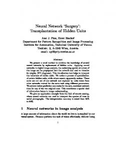
3: Black Box Experiments In the black box experimental context we attempted to train a neural network to associate direct measures from an Ada package specification with a corresponding set of reusability ratings for that package. The training set contained 256 vectors while the test set 25 vectors. In constructing the data for an experiment, each vector contained up to 16 inputs and 5 outputs to choose from, including: • number of procedures or functions, • uncommented lines (number of lines that contain Ada source code not followed by a comment on the same physical line [8]), • physical comment lines (number of lines that contain only a comment -- no legal Ada appears on the line [8]), • extent of genericity (number of parameters passed to a generic package), • SLOC (number of lines ending with a semi-colon [8]), • physical size (summation of physical ada lines, physical comment lines, and physical blank lines [8]), and • file size (byte size of a package on a UNIX platform). The input parameters group roughly as size, coupling, and adaptability. The input space was modified over several experiments. The intent was twofold: to determine sensitivity of the different parameter types, and to see if repeating the same type of parameter would boost performance. The output parameters contained four user assessments and an average of the four ratings. We varied the output parameter space to look at 1) how well the neural network trained on individual ratings, 2) how well it trained on an average of the four ratings, and 3) all five ratings (based on the Yu and Simmons argument [19] that the more information you can provide in the output parameter space, the better the neural network will train). We also varied the number of epochs, neural network architecture, and number of vectors in the training set. Figure 1 is indicative of the black box experiments performed. The learning rate (alpha) and number of epochs is self-explanatory, but the neural net (NN) architecture may not be; “5+5+5+1” denotes a network with five inputs, two hidden layers of five nodes each which are fully connected beyond hidden layers to 2 layers before or after (pluses ACOSM’93, Nov. 18-19 ‘93
3
5+5+5+1 NN architecture, 17,000 epochs, Alpha is .05 1
0.75
0.5
0.25 Desired results Actual results 0 0
0.25
0.5
0.75
1
Figure 1: Black Box example denote interconnection of non-adjacent layers, minuses denote interconnection of adjacent layers only), and one output node. The hash marks on the diagonal line represent where expected values ought to have occurred. Each error bar represents one of five classes of test vectors. Tic marks are values predicted by the neural network for a given class. Ideally, all tic marks would gravitate towards the hash marks rather than fall above or below the expected values on the diagonal line. The results show a large variance for each error-bar. Also, values on the error-bars show little gravitation towards ideal values -- suggesting little if any correlation between actual and desired values. If a highly correlated pattern had emerged, the error bars would have appear in a stair stepping formation. By nature, a specification provides the “what” instead of the “how” of a component. This basically left us only 5 input parameters with which to work: SLOC, number of generic parameters, number of procedures and functions, percent documentation, and number of withs. All other input parameters conveyed essentially the same information. The lack of detail also seemed to generate a lot of noise in the training set so that two identical sets of input parameters were associated with two different output ratings. There did not seem anyway around these problems, so we moved on to white-box testing to see if we could fare better.
4: White Box Experiments The white box experiments attempted to correlate measures extracted from Ada bodies to corresponding assessments. The training set contained 424 vectors, while the test set contained 25 vectors. The inputs came from one of four major classes, complexity, volume, coupling, and size. The Volume parameters corresponded to both unique and total number of operators and operands (4 in all) which normally associated with Halstead’s metrics. Cyclomatic complexity consisted of a package body’s edges, nodes, and number of procedures win a package. Coupling was the number of “withs” from a standard library or from a user defined library. Size was the physical lines of code, number of executable statements and the number of comments, and total number of bytes. They were defined as follows: Physical lines were the actual number of lines of source code, number of executable statements used the number of semi-colons; and number of comments counted any line that had a comment (even if the line also contained executable code). Total number of bytes was the source file size. The output parameters contained four user assessments and an average of the four ratings as in the black box experiments. Once again the output parameter space was varied to examine 1) differences in correlations over individual
ACOSM’93, Nov. 18-19 ‘93
4
15-15-15-1 NN architecture, 20,000 epochs, Alpha is .02 1
0.8
0.6
0.4
0.2 Desired value along the Diagonal line Actual Value in the form of error bars 0
0
0.25
0.5
0.75
1
Figure 2: White Box Results ratings, 2) training on the rating average, and 3) training on all five output parameters. Table 2 shows the layout for a typical test suite. Table 2: Layout for Input and Output Parameters Complexity
Edges
Nodes
# of Modules
Vocabulary
n1
N1
n2
Size
N2
SLOC
No. of Exec. lines
# of Comment lines
Coupling
File Size
# of withs (lib)
# of withs (user)
Assigned Rating
Vector 1 : Vector N For the white box experiment we also varied the size of the neural network training set, input parameter space, neural network learning rate (alpha), and neural network architecture. Figure 2 shows the results from an experiment using 424 training vectors and 25 test vectors. The experiment ran for 20,000 epochs in a 15-15-15-1 neural network configuration. Ideally, the error bars should collapse upon the desired values along the diagonal ideal. Instead, the error bar progression show little definitive shape and more variance than desired. Since the assessment rating average provided few dividends, we devised another experiment associating input values with the assessment ratings of each of the individual assessors (see figure 3). Each subgraph shows how well the neural network predicted a particular assessor’s ratings. The origin represents where all artifacts rated non-reusable (i.e., those assigned a value of zero) should appear. The error bar above the origin represent how well the neural netACOSM’93, Nov. 18-19 ‘93
5
14-12-12-1 NN architecture, 1000 epochs, Alpha is .02
Reader A
Reader B
Reader C
Reader D
1
1
1
1
0.5
0.5
0.5
.5
0
0
0
0
0
1
0
1
0
1
0
1
Figure 3: Individual assessments of 20 test vectors (10 rated 0, 10 rated 1) work predicted this event for each assessor. The point (1,1) is where all artifacts rated reusable (i.e., those assigned a value of one) should appear. The error bar below this point is what the neural network predicted for code assessed as reusable. Overall, the results are fairly positive. Success (defined as rounding to the expected results of 0 or 1) ranged from 65 percent (reader A) to 80 percent accuracy (reader C). The clustering and variance are worth noting in the graphs. For example, reader C had good clustering near the desired points, but some points strayed far from the mark. This last set of results provided some promise, so we decided to investigate a combination of black box and white box, which we shall refer to as grey box experiments.
5: Grey Box Experiments The intent of this experiment is to determine whether combining black and white input parameters yields better results. Viewing an artifact as a grey box seems most realistic since it gives developers the choice of either verbatim or adaptive reuse, depending on circumstances. A well designed artifact may provide enough flexibility through genericity, but due to unforeseen hardware changes a developer may want the capability to adapt the artifact. Initially we started with all the input parameters from the white box experiments and extended the input parameter set with black box parameters: extent of genericity, physical lines, and total number of “withs.” These three parameters correspond well with the reuse features of adaptability, complexity, and coupling. The output set consisted of the averages from the white box ratings. Also, we eliminated those artifacts that contained different black box and white box assessment averages. At the start of this experiment the test set contained only twenty vectors. Results generated seemed good, so we enlarged the test set to forty vectors in order to better validation the initial results. The forty vectors formed five groups of eight vectors where the five groups provided complete and balanced coverage of all possible outcomes We ran several experiments, varying neural net architecture, learning rate, and number of epochs. Figure 4 shows the results of the experiment running for 2,000 epochs, using a neural network with one hidden layer of sixteen units and a learning rate of 0.02. The error bars cluster reasonably well near the desired points on the diagonal line. There is tighter clustering near the end points. This behavior matches well with the consensus among readers on artifact ratings at these extremes. ACOSM’93, Nov. 18-19 ‘93
6
16-16-1 NN architecture, 2000 epochs, Alpha is .02 1
0.75
0.5
0.25 Diagonal: Desired results Error Bars: Actual results 0 0
0.25
0.5
0.75
1
Figure 4: Grey Box testing 15-15-15-1 NN architecture, 6 programs, Alpha is .02 1
0.8
0.6
0.4 After 50 epochs After 100 epochs After 300 epochs After 400 epochs After 1400 epochs
0.2
0 1
2
3
4
5
6
Figure 5: Neural net training of Tracz’s reuse examples As a final test we constructed a test set from six Ada procedures developed by Tracz [17] (see Appendix A for actual code). These programs were specifically designed to be demonstrate syntactic ways of improving code for reusability. The input set contained all 449 vectors assessed during white box test. Since the examples were procedures and not packages, we added only one black box parameter to the white box mix, the extent of genericity. Note that only one of the four assessors had any significant exposure to Tracz’s paper prior to the experiments, and the programs were not brought into the experiments until after the assessors were completed with their assessments of the other samples. Assessment of Tracz’s programs therefore provides an objective validation of our work. Figure 5 shows the results generating from analyzing Tracz’s programs. Each line represents progression of the neural network through a number of epochs. Each tic-mark on the X-axis represents the corresponding Tracz prograACOSM’93, Nov. 18-19 ‘93
7
m.Observe that the line shape generated remained stable throughout all the epochs. This suggests that the general shape of the line emerges with relatively minimal training. The general line patterns seem very plausible and supportive of the neural network approach.
6: Discussion Without statistical support for our work, much of our commentary borders on vigorous hand-waving. Table 3 lists the significance of our results. The black box results of figure 1 show little correlation to the expected values. The statistics look better for the white box results of figure 2, but they are not exactly desirable. The grey box experiments of figure 4 produce the best statistical results, demonstrating the synergistic effect that two poorly performing models can generate jointly. These numbers, especially the correlation coefficient, are statistically significant and indeed support the neural network approach as a viable paradigm in constructing metrics. Table 3: Analysis of Experiments Experiment
R-squared
Correlation
Black Box
.03
.18
White Box
.32
.57
Grey Box
.75
.86
The progression of results through the three experiments and the external validation of those results with Tracz’s examples demonstrates the simplicity and the power of neural approaches to measurement. The simplicity comes in the relatively direct nature of our inputs, as compared to other approaches to reusability assessment. The power comes in the ability to employ relative novices as trainers for the network. It is not necessary (or perhaps even desirable!) to employ too much expertise in measurement or in reuse in the derivation of a measure that must reflect a typical programmer’s ability to reuse existing software components. The performance of the network on Tracz’s examples is particularly noteworthy in two areas. First, the network was trained primarily on packages, whereas Tracz’s examples are all procedures. This implies that the network is reasonably robust in its evaluation, as we would expect from the nature of its inputs. Second, the network generates results after 50 epochs that are substantially similar to the results generated after 1400 epochs, implying that there is no requirement for substantial computational overhead in the production use of the technique.
7: Conclusions We have demonstrated the derivation of a reusability metric through neural networks, and further shown that the network is capable of robust evaluation of material for which it was not specifically trained. This approach supports intuitive assessment of artifacts without excessive concern for the derivation of polynomials to model the desired function. Looking towards the future there are several directions to proceed. These include improving sensitivity analysis and application of the approach in different contexts. Greater sensitivity analysis could be performed on the output parameters. The assessment could be expanded from a binary to an ordinal scale. This would give assessors greater accuracy in expressing their selection. Second, additional assessment questions could be included which address reusability issues at a finer granularity level. Sensitivity analysis could also be applied to the input parameters. For example, unconstrained array usage may be an important factor to include. Applying the approach to different contexts could prove invaluable. Obviously, there are many metrics which exist that do not have a mathematical model [14]. Our approach could generate a neural network models for metrics where no mathematical model exists. The neural network paradigm could be applied to other programming languages to develop appropriate metrics. This process could be applied to other artifacts in the software life cycle whether they be product or process in nature. Currently, some of these directions are under investigation.
ACOSM’93, Nov. 18-19 ‘93
8
Software reuse is here to stay. Organizations that adopt a mature approach to software engineering will find formal reuse a part of their process. If they desire to effectively reuse the intellectual capital buried with their legacy code an efficient process of reuse assessment needs to be established. A cornerstone to this process is a method for characterizing reusable software. Using a neural network approach to characterize software can potentially be that cornerstone.
Acknowledgments The authors would like to thank Alan Dennis, W. Keith Jones, David Carvell, Pratibha Kattemalavadi, and Edward Tennant for their assistance in test suite construction, artifact assessment, and experiment generation.
References [1]
Biggerstaff, T. J. and Perlis, A. J., “Forward: Special Issue on Software Reusability”, IEEE Transactions on Software Engineering, Vol. SE-10, No. 5, September 1984, pp. 474-476.
[2]
Boetticher, G., K. Srinivas and D. Eichmann, “A Neural Net-Based Approach to Software Metrics,” Proc. of the 5th International Conference on Software Engineering and Knowledge Engineering, 1993, pp. 271-274.
[3]
Braun, C. L., J. B. Goodenough and R. S. Eanes, “Ada Reusability Guidelines”, Tech. report 3285-2-208/2, SofTech, Inc., April 1985.
[4]
Burton, B. A., “A Practical Approach to Ada Reusability”, Proceedings of National Conference on Software Reusability and Maintainability, September 10-11 1986.
[5]
Caldiera, G. and V. R. Basili, “Identifying and Qualifying Reusable Software Components,” IEEE Computer, Vol. 24, No. 2 February 1991, pp. 61-70.
[6]
Card, D., V. Church and W. Agresti, “An Empirical Study of Software Design Practices,” IEEE Transactions on Software Engineering, Vol. SE-12, No. 2, February 1986, pp. 264-271.
[7]
Dillehunt, D., N. S. Nise and C. Giffin, “Reusable Software Development”, Rockwell International.
[8]
Dynamics Research Corporation, AdaMAT Reference Manual, 1992.
[9]
Fahlman, S. E. and M. Lebiere, An Empirical Study of Learning Speed in Back-Propagation Networks, Tech Report CMU-CS-88-162, Carnegie Mellon University, September, 1988.
[10] Grady, R. and D. Caswell, Software Metrics: Establishing a Company-Wide Program, Englewood Cliffs, NJ: Prentice-Hall, Inc., 1987. [11] Jones, T. C., “Reusability in Programming: A Survey of the State of the Art,”, IEEE Transactions on Software Engineering, Vol. SE-10, No. 5, September, 1984, pp. 488-493. [12] Lanergan, R. G. and C. A. Grasso, “Software Engineering with Reusable Design and Code”, IEEE Transactions on Software Engineering, Vol. SE-10, No. 5, September, 1984, pp. 498-501. [13] Litvintchouk, S. D., and A. S. Matsumoto, “Design of Ada Systems Yielding Reusable Components: An Approach Using Structured Algebraic Specification”, IEEE Transactions on Software Engineering, Vol. SE-10, No. 5, September 1984, pp. 544-551. [14] Oh, S. H., Y. J. Lee and M. H. Kim, “A Management Discipline of Software Metrics and the Software Quality Manager,” International Journal of Software Engineering and Knowledge Engineering, Vol. 2, No. 3, September 1992, pp. 449-465. [15] Paulk, M. C., B. Curtis, M. B. Chrissis and C. V. Weber, “Capability Maturity Model, Version 1.1”, IEEE Software, Vol. 10, No. 4, July 1993, pp. 18-27. [16] Polak, W., “Maintainability and Reusable Program Designs”, Proceedings of National Conference on Software Reusability and Maintainability, September 10-11, 1986. [17] Tracz, W., “Parameterization: A Case Study”, ACM AdaLetters, Vol. 9, No. 4, May/June 1989. [18] Wegner, P., “Varieties of Reusability”, Proceedings of ITT Workshop on Reusability in Programming, September 7-9, 1983. [19] Yu, Y.-H., and R. F. Simmons, Extra Output Biased Learning, Tech Report AI90-128, University of Texas at Austin, March, 1990. ACOSM’93, Nov. 18-19 ‘93
9
Appendix A — Tracz’s Series of Programs procedure sample1 is Max : Integer; A: array (1..10) of Integer;{ -- Find the Largest Value in A begin Max:=0; for I in 1..10 loop if Max < A(I) then Max := A(I); -- Find a new largest value end if; end loop; end sample1; -----------------------------------------------------------------------procedure sample2 is type Element is new Integer; -- New type Vector is array (Integer range 1..10) of Element; Max : Element; A: Vector; -- Find the largest value in a begin Max:= A(A’First); for I in A’Range loop if Max < A(I) then Max:= A(I); end if; end loop; end sample2; -----------------------------------------------------------------------Procedure sample3 is type element is range 0..100; -- changed type vector is array (integer range ) of element; -- changed max : Element; A : vector (1..10); -- changed B : vector (0..99); -- new - assume a blah blah blah function Find_the_Max_of(the_Array: in vector) return Element is Max:Element:= The_Array(The_Array’First); -- changed begin for I in The_Array’First+1.. The_Array’Last loop --changed if Max < The_Array(I) then Max:= The_Array(I); end if; end loop; return Max; end Find_the_Max_of; begin null; end sample3; -----------------------------------------------------------------------procedure sample4 is type element is range 0..100; -- changed type vector is array (integer range ) of element; -- changed max : Element; A : vector (1..10); -- changed B : vector (0..99); -- new addition Null_Array:exception; function Find_the_Max_of(The_Array: in Vector) return Element is Max:Element; --changed begin if The_Array’Length = 0 then --New raise Null_Array; --new end if; Max:= The_Array(The_Array’First); --New for I in The_Array’First+1.. The_Array’Last loop --changed if Max < The_Array(I) then Max:= The_Array(I); end if; end loop; return Max; end Find_the_Max_of; begin
ACOSM’93, Nov. 18-19 ‘93
10
null; end sample4; -----------------------------------------------------------------------generic type Element is limited private; type Index is (); type Vector is array (Index range ) of Element; with function “ --| (exist I: The_Array’Range=. he_Array(I) = Z) and --| (for all I: The_Array’Range => The_Array(I) First_Index_of(The_Vector)); Assign(Into => Last_Index, From => last_Index_of(The_Vector)); Assign(Into => Max, From => Get_ELement(The_Vector,Current_Index)); while Current_index /= Last_Index loop Assign(Into => Current_Index, From => Next_Index(Current_Index)); Assign(The_Current_Element,Get_Element(The_Vector,Current_Index)); if Max < The_Current_Element then Assign(Into=>Max,From=>The_Current_Element); end if; end loop; return Max; end Find_the_Max_of;
ACOSM’93, Nov. 18-19 ‘93
11