A Neuromorphic VLSI System for Modeling Spike

Diss. ETH No. 16578

A Neuromorphic VLSI System for Modeling Spike–Based Cooperative Competitive Neural Networks

A dissertation submitted to the SWISS FEDERAL INSTITUTE OF TECHNOLOGY (ETH ZURICH) for the degree of Doctor of Natural Sciences presented by ELISABETTA CHICCA Dipl.-Phys. Universit`a di Roma “La Sapienza” born April 1, 1972 citizen of Rome, Italy accepted on the recommendation of Prof. Dr. Rodney J. Douglas, examiner Dr. Giacomo Indiveri, co-examiner Dr. Daniel Kiper, co-examiner 2006

Abstract Neuromorphic engineering is an emerging research field which explores methodologies for implementing biologically inspired systems in hardware. It has a key role in neuroscience as a means for testing hypotheses concerning the computation carried out by the brain, while at the same time it promotes the development of artificial systems capable of achieving performance figures comparable to those of biological neural systems. I am interested in applying neuromorphic engineering methods as a tool for understanding cortical computation and its relation to recurrent intra-cortical connectivity. This thesis describes the development and testing of a neuromorphic VLSI implementation of a spiking recurrent cortical network model and the hardware/software infrastructure required to operate it. The local connectivity of my neural network is an abstract representation of the cooperative–competitive connectivity observed in cortex, which is believed to play a major role in shaping cortical responses and selecting the relevant signal among distractors and noise. The hardware/software infrastructure allows us to build multi–chip systems, to configure the inter–chip and intra–chip connectivity, to provide external stimuli to the multi–chip system and to monitor the activity of all chips, providing a highly flexible tool for testing complex systems. I performed software simulations and real–time experiments with the working chip to demonstrate that the spiking network exhibits the complex behaviors predicted by well known theoretical studies on more abstract models (e.g. dynamic field theory, rate model) of similar architectures. I carried out experiments with both artificially generated, well controlled stimuli and “real” sensory data generated by a silicon retina chip. In the latter case, I implemented (in collaboration with my collegue Patrick Lichtsteiner) and tested a two chip vision based system for exploring computational models of feature selectivity in a realworld scenario, and so demonstrated the feasibility of real-time inter-chip communication through our hardware/software infrastructure. Such a feasibility proof is a necessary step for evolving the neuromorphic systems developed so far into complex and scalable systems endowed with sophisticated computational capabilities. The VLSI spiking recurrent network and the hardware/software infrastructure described in this thesis provide a highly flexible platform to test the computational properties of cooperative competitive neural networks in real–time, and allows us to test the role of spike timing with real–world stimuli. The insights gained through with this work, the technology developed and the methodologies derived provide an important stepping stone toward the understanding and practical application of recurrent, cooperative–competitive neural networks.

i

ii

Abstract

Keywords: neuromorphic, VLSI, neural networks, Integrate–and–Fire (I&F) neuron, Address Event Representation, cooperative competitive networks, orientation selectivity.

Prefazione L’ingegneria neuromorfa e` un campo di ricerca emergente che esplora le metodologie per progettare sistemi fisici prendendo ispirazione dalla biologia. Essa ha un ruolo fondamentale come mezzo per valutare ipotesi riguardo la computazione eseguita dal cervello e, allo stesso tempo, promuove lo sviluppo di sistemi artificiali capaci di raggiungere prestazioni confrontabili a quelle dei sistemi neurali biologici. Il mio interesse principale riguarda l’utilizzo delle metodologie dell’ingegneria neuromorfa come strumento per comprendere i processi computazionali che avvengono nella corteccia cerebrale e la loro relazione con la connettivit`a ricorrente corticale. Questa tesi descrive lo sviluppo e l’analisi di una trasposizione in VLSI neuromorfo di un modello di rete ricorrente corticale e l’infrastruttura hardware/software per farla funzionare. La connettivit`a locale della rete neurale rappresenta in modo astratto la connettivit`a di natura cooperativa e competitiva presente nella corteccia cerebrale, la quale si pensa abbia un ruolo fondamentale nel plasmare l’attivit`a corticale e nell’amplificare i segnali che codificano l’informazione, sopprimendo quelli che derivano da distrattori e rumore. L’infrastruttura hardware/software sviluppata ci permette di costruire sistemi multi–chip, configurare la connettivit`a inter–chip ed intra–chip, fornire stimoli esterni al sistema multi– chip e monitorare l’attivit`a di tutti i chip, fornendo cos`ı uno strumento flessibile per testare sistemi complessi. In questo lavoro ho eseguito simulazioni software ed esperimenti con il chip in tempo reale per dimostrare che la rete neurale artificiale esibisce gli stessi comportamenti complessi descritti da studi analitici su modelli di architetture simili. In questi esperimenti la rete ricorrente e` stata stimolata sia con stimoli generati artificialmente sia con stimoli percettivi “reali” generati da una retina artificiale. In quest’ultimo caso, ho realizzato e caratterizzato (in collaborazione con Patrick Lichtsteiner) un sistema visivo composto da due chip per studiare possibili modelli computazionali per la selettivit`a a caratteristiche dello stimolo visivo (come ad esemprio, orientamento) in uno scenario realistico. Questo sistema dimostra la funzionalit`a della comunicazione tra chip in tempo reale attraverso l’infrastruttura sviluppata. Questa prova di funzionalit`a rappresenta un passo fondamentale per lo sviluppo di sistemi neuromorfi in architetture complesse e scalabili dotate di propriet`a computazionali elaborate. La rete VLSI ricorrente realizzata con neuroni integrate–and–fire e l’infrastruttura hardware/software descritte in questa tesi costituiscono uno strumento flessibile per indagare le propriet`a computazionali delle reti neurali, cooperative e competitive, in tempo reale e permette di verificare ipotesi riguardo al ruolo delle temporizzazioni tra gli impulsi

iii

iv

Prefazione

neuronali attraverso l’uso di stimoli realistici. I risultati ottenuti con questo lavoro, la tecnologia sviluppata e la metodologia proposta rappresentano un ulteriore passo verso la comprensione e l’applicazione pratica delle reti neurali competitive e cooperative. Parole chiave: neuromorfo, VLSI, reti neurali, neurone Integrate–and–Fire (I&F), Address Event Representation (AER), reti cooperative e competitive, selettivit`a all’orientamento.

To Daniele and Giulia

v

Contents Abstract

i

Prefazione

iii

1 Introduction 1.1 Motivation . . . . . . . . . . . . . . . . . . . . . . . . . . . . . . . . . . . 1.2 Outline of this Thesis . . . . . . . . . . . . . . . . . . . . . . . . . . . . .

1 1 3

2 The Address–Event Representation and Event–Based Neuromorphic Systems 2.1 The Address–Event Representation . . . . . . . . . . . . . . . . . . . . . . 2.2 Analysis of Time Multiplexing Techniques . . . . . . . . . . . . . . . . . . 2.2.1 Sequential Scanning . . . . . . . . . . . . . . . . . . . . . . . . . 2.2.2 ALOHA Access Protocol . . . . . . . . . . . . . . . . . . . . . . . 2.2.3 Priority Encoder . . . . . . . . . . . . . . . . . . . . . . . . . . . 2.2.4 Arbitrated Access . . . . . . . . . . . . . . . . . . . . . . . . . . . 2.2.5 Summary . . . . . . . . . . . . . . . . . . . . . . . . . . . . . . . 2.3 Arbitrated AER for Multi–chip Systems . . . . . . . . . . . . . . . . . . . 2.4 AER Hardware Infrastructures . . . . . . . . . . . . . . . . . . . . . . . . 2.5 The PCI–AER Hardware Infrastructure . . . . . . . . . . . . . . . . . . . 2.5.1 The PCI–AER Board . . . . . . . . . . . . . . . . . . . . . . . . . 2.5.2 Supporting Software . . . . . . . . . . . . . . . . . . . . . . . . .

5 5 6 8 9 10 10 11 12 14 15 15 20

3 Analog Circuits for Implementing Spike Based Processing Models 3.1 Subthreshold MOSFET Characteristic . . . . . . . . . . . . . . 3.2 Differential Pair and Transconductance Amplifier . . . . . . . . 3.3 Capacitive Voltage Divider . . . . . . . . . . . . . . . . . . . . 3.4 Current Mirror . . . . . . . . . . . . . . . . . . . . . . . . . . 3.5 Current Mirror Integrator . . . . . . . . . . . . . . . . . . . . . 3.5.1 Response to Spike Trains: Approximate Solution . . . . 3.5.2 Response to Spike Trains: General Analytical Solution . 3.6 Excitatory and Inhibitory Synapses . . . . . . . . . . . . . . . . 3.7 The Adaptive Synapse . . . . . . . . . . . . . . . . . . . . . . 3.7.1 Experimental Results . . . . . . . . . . . . . . . . . . . 3.8 The Integrate–and–Fire Silicon Neuron . . . . . . . . . . . . .

23 23 25 28 29 30 31 33 34 34 38 41

vii

. . . . . . . . . . .

. . . . . . . . . . .

. . . . . . . . . . .

. . . . . . . . . . .

. . . . . . . . . . .

. . . . . . . . . . .

viii

Contents 3.9

4

5

6

7

Discussion . . . . . . . . . . . . . . . . . . . . . . . . . . . . . . . . . . .

Cooperative–Competitive Neural Networks 4.1 Analytical Methods Applied to Cooperative–Competitive Networks 4.2 The Neural Code . . . . . . . . . . . . . . . . . . . . . . . . . . . 4.3 Neural Coding in Ring of Neurons Competitive Networks . . . . . . 4.4 Software Simulation of the Ring of Neurons Competitive Network . 4.4.1 Sharpening and Suppression of Less Effective Stimuli . . . 4.4.2 Hysteretic Behavior . . . . . . . . . . . . . . . . . . . . . 4.5 Discussion . . . . . . . . . . . . . . . . . . . . . . . . . . . . . . .

. . . . . . .

. . . . . . .

. . . . . . .

. . . . . . .

44 45 47 50 51 53 53 55 56

VLSI Competitive Networks of Spiking Neurons 5.1 The IFRON Chip: a VLSI Implementation of a Spiking Cooperative Competitive Network . . . . . . . . . . . . . . . . . . . . . . . . . . . . . . . . 5.1.1 Chip Architecture . . . . . . . . . . . . . . . . . . . . . . . . . . . 5.1.2 Circuits . . . . . . . . . . . . . . . . . . . . . . . . . . . . . . . . 5.2 IFRON Chip Experiments . . . . . . . . . . . . . . . . . . . . . . . . . . 5.2.1 Basic Building Blocks Behavior . . . . . . . . . . . . . . . . . . . 5.2.2 Basic Network Behavior . . . . . . . . . . . . . . . . . . . . . . . 5.2.3 Sharpening and Suppression of Least Effective Stimuli . . . . . . . 5.3 Discussion . . . . . . . . . . . . . . . . . . . . . . . . . . . . . . . . . . .

59

A Multi-Chip Neuromorphic System for Feature Selectivity 6.1 Orientation Selectivity Using a Silicon Retina and the IFRON chip 6.1.1 The TMPDIFF Chip . . . . . . . . . . . . . . . . . . . . 6.2 Orientation Selectivity Experiments . . . . . . . . . . . . . . . . 6.3 Discussion . . . . . . . . . . . . . . . . . . . . . . . . . . . . . .

. . . .

83 87 87 88 95

Conclusions 7.1 Ideas for Further Work and Outlook . . . . . . . . . . . . . . . . . . . . .

97 99

. . . .

. . . .

. . . .

. . . .

61 62 66 72 72 74 75 81

A The M/G/1 Queue and the Pollaczek-Khinchin formula

101

B PCI-AER Library Interface Specification B.1 Introduction . . . . . . . . . . . . . . . . . . . . . . . . . . . . . . . B.2 Description of the PCI–AER Library Functions . . . . . . . . . . . . B.2.1 Common Functions Applicable to More Than One Sub-device B.2.2 Monitor Sub–device . . . . . . . . . . . . . . . . . . . . . . B.2.3 Sequencer Sub-device . . . . . . . . . . . . . . . . . . . . . B.2.4 Mapper Sub-device . . . . . . . . . . . . . . . . . . . . . . .

103 103 103 103 105 108 110

. . . . . .

. . . . . .

. . . . . .

C IFRON Software Simulation Tool

115

D Arbiter UPI Code

117

Contents

ix

Abbreviations and Symbols

135

Bibliography

137

Curriculum Vitae

147

List of Figures 2.1 2.2 2.3 2.4 2.5 2.6 2.7 3.1 3.2 3.3 3.4 3.5 3.6 3.7 3.8 3.9 3.10 3.11

Schematic diagram of an AER chip–to–chip (adapted from [37]). . . . . . . . . . . . . . . . Merit criterion versus number of cells for three (adapted from [33]). . . . . . . . . . . . . . . . Point–to–Point handshake protocol. . . . . . . SCX handshake protocol. . . . . . . . . . . . . PCI–AER board. . . . . . . . . . . . . . . . . PCI–AER header board. . . . . . . . . . . . . Block diagram of the PCI–AER interface board.

communication example . . . . . . . . . . . . . . . different access protocols . . . . . . . . . . . . . . . . . . . . . . . . . . . . . . . . . . . . . . . . . . . . . . . . . . . . . . . . . . . . . . . . . . . . . . . . . . . . . . . . . . . . . . . . . .

3.17

Schematic drawing of the physical structure of an n–type MOS transistor. . Symbols for an n–type MOS transistor and a p–type MOS transistor. . . . . The current Ids as a function of Vds . . . . . . . . . . . . . . . . . . . . . . Schematic diagram of the differential pair. . . . . . . . . . . . . . . . . . . Transconductance amplifier. . . . . . . . . . . . . . . . . . . . . . . . . . Capacitive voltage divider. . . . . . . . . . . . . . . . . . . . . . . . . . . Current mirror. . . . . . . . . . . . . . . . . . . . . . . . . . . . . . . . . Current Mirror Integrator (CMI). . . . . . . . . . . . . . . . . . . . . . . . Schematic diagram of the excitatory synapse. . . . . . . . . . . . . . . . . Schematic diagram of the adaptive synapse. . . . . . . . . . . . . . . . . . Voltages across the facilitating capacitor Cf and the depressing capacitor Cd in response to a 50 Hz spike train (analytical derivation). . . . . . . . . Output current of the adaptive synapse in response to a 50 Hz spike train (plot of the analytical expression of the current). . . . . . . . . . . . . . . . Schematic diagram of the chip architecture. . . . . . . . . . . . . . . . . . Steady state amplitude of the EPSP as a function of presynaptic frequency for three different values of V wf . . . . . . . . . . . . . . . . . . . . . . . . Steady state amplitude of the EPSP as a function of presynaptic frequency for six different values of V wd . . . . . . . . . . . . . . . . . . . . . . . . . Normalized EPSP amplitude in response to the first ten pulses of a 20Hz train of spikes for three different values of V wd . . . . . . . . . . . . . . . . Schematic diagram of the integrate–and–fire neuron. . . . . . . . . . . . .

4.1 4.2

Schematic representation of the ring–of–neurons architecture. . . . . . . . Feature tuning curve sharpening. . . . . . . . . . . . . . . . . . . . . . . .

3.12 3.13 3.14 3.15 3.16

xi

7 12 13 13 16 17 18 24 25 26 27 27 28 29 30 35 35 37 37 39 40 40 41 42 52 54

xii

List of Figures 4.3 4.4

Suppression of less effective stimuli. . . . . . . . . . . . . . . . . . . . . . Hysteretic behavior. . . . . . . . . . . . . . . . . . . . . . . . . . . . . . .

55 56

5.1 5.2 5.3 5.4 5.5 5.6 5.7 5.8 5.9 5.10 5.11 5.12

Chip layout legend. . . . . . . . . . . . . . . . . . . . . . . . . . . . . . . IFRON chip architecture and schematic representation. . . . . . . . . . . . IFRON chip layout and photograph. . . . . . . . . . . . . . . . . . . . . . IFRON layout. . . . . . . . . . . . . . . . . . . . . . . . . . . . . . . . . Layout of the I&F neuron. . . . . . . . . . . . . . . . . . . . . . . . . . . Layout of the adaptive synapse. . . . . . . . . . . . . . . . . . . . . . . . . Handshaking circuit for the AER input. . . . . . . . . . . . . . . . . . . . Layout of the AER input decoder. . . . . . . . . . . . . . . . . . . . . . . Layout of the AER output. . . . . . . . . . . . . . . . . . . . . . . . . . . The one–dimensional voltage scanner. . . . . . . . . . . . . . . . . . . . . The IFRON chip test setup. . . . . . . . . . . . . . . . . . . . . . . . . . . Network response to homogeneous constant input current with all synaptic connections disabled. . . . . . . . . . . . . . . . . . . . . . . . . . . . . . Membrane potentials. . . . . . . . . . . . . . . . . . . . . . . . . . . . . . Strong WTA behavior. . . . . . . . . . . . . . . . . . . . . . . . . . . . . Traveling wave. . . . . . . . . . . . . . . . . . . . . . . . . . . . . . . . . Raster plot of the input stimulus used in the sharpening experiment. . . . . Raster plot of the activity of the feed–forward network in response to the stimulus shown in Fig. 5.16. . . . . . . . . . . . . . . . . . . . . . . . . . Sharpening. . . . . . . . . . . . . . . . . . . . . . . . . . . . . . . . . . . Raster plot for the suppression experiment: feed–forward network response. Raster plot for the suppression experiment: recurrent network response. . . Suppression for three different values of global inhibition. . . . . . . . . . Suppression for several values of lateral excitation. . . . . . . . . . . . . .

61 63 64 65 67 67 68 68 70 71 73

5.13 5.14 5.15 5.16 5.17 5.18 5.19 5.20 5.21 5.22 6.1 6.2 6.3 6.4 6.5 6.6 6.7

Feed–forward model of the organization of simple receptive fields (adapted from [59]). . . . . . . . . . . . . . . . . . . . . . . . . . . . . . . . . . . . AER vision system setup. . . . . . . . . . . . . . . . . . . . . . . . . . . . AER vision system setup (photograph). . . . . . . . . . . . . . . . . . . . Integrated response of the silicon retina to oriented flashing bars . . . . . . Tuning curves for the feed–forward and the feed–back model of orientation selectivity. . . . . . . . . . . . . . . . . . . . . . . . . . . . . . . . . . . . Tuning curves for the feed–forward and the feed–back model of orientation selectivity for the neuron with vertical preferred orientation. . . . . . . . . Population data. . . . . . . . . . . . . . . . . . . . . . . . . . . . . . . . .

74 75 76 76 77 77 78 79 79 80 80 85 89 89 90 91 92 93

A.1 Evolution of the residual service time over time. . . . . . . . . . . . . . . . 102 C.1 Structure of variables used in the IFRON software simulation tool. . . . . . 116

List of Tables 2.1

Summary of the characteristics of four access algorithms for AE communication channels. . . . . . . . . . . . . . . . . . . . . . . . . . . . . . . . .

11

5.1

Characteristics of the spiking WTA networks described in the literature. . .

60

6.1

Parameters obtained by least–squares fitting of the data to the von Mises distribution. . . . . . . . . . . . . . . . . . . . . . . . . . . . . . . . . . .

94

xiii

Chapter 1

Introduction “As engineers we would be foolish to ignore the lessons of a billion years of evolution” - Carver Mead, 1993

1.1 Motivation Biological systems perform complex processing tasks on a scale and speed that can not be achieved by conventional digital computers. Machine simulation of human functions has been a challenging research field since the advent of digital computers. Despite the resources dedicated to this field, humans still outperform the most powerful computers in relatively routine functions such as vision. For example, in spite of about 50 years of research in the field of pattern recognition, the general problem of recognizing complex visual patterns with arbitrary orientation, location and scale remains largely unsolved [67]. Artificial systems have been implemented to solve more specific tasks in the field of pattern recognition, for example, the problem of character recognition. Machine simulation of character recognition has been the subject of intensive research for the last three decades, yet it is still far from achieving performances comparable with those of humans [8]. Computation in biological systems is based on completely different principles from those used in conventional digital computers. The disparity between the effectiveness of computation in the nervous system and in a computer is primarily attributable to the way the elementary devices are used in the systems, and to the kind of computational primitives they implement [87]. In digital systems the elementary devices are transistors whose physical properties are not exploited as computational primitives: the representation of information relies on digital values, ignoring the analog nature of transistors. The elementary operations, or computational primitives, are usually the logical operations AND, OR, and NOT. Neuromorphic engineering plays a key role in the development of artificial systems capable of achieving performance figures comparable to those of the biological neural systems. This emerging research field is a methodology for implementing biologically inspired devices, comprised of artificial neurons and synapses, and combinations of sensory and computational modules in hardware. The term neuromorphic was coined by Carver Mead in the late ’80s to describe Very Large Scale Integration (VLSI) systems comprised of ana-

1

2

Chapter 1. Introduction

log circuits and built to mimic biological neural cells and architectures [88]. The main idea behind neuromorphic engineering is to implement the same basic operations as those of the nervous system starting from the elementary operations defined by transistor device physics. Mead pointed out that the same physical principles apply to the conductance of a transistor operated in subthreshold and to the macroscopic conductance of a population of voltage–gated channels1 , giving rise to an exponential dependence on the applied voltage in both cases. Implementing artificial neural systems to perform specific tasks is not the only aim of neuromorphic engineering. Neuroscience can take advantage of full–custom neuromorphic integrated circuits as a means for testing hypotheses concerning the computation carried out by the brain. The neocortex is often considered the relevant brain structure in studying the evolution of intelligence because higher cognitive abilities are generally associated with neocortical functions, and primate encephalization is primarily a result of increased neocortical size [45, 68, 104]. Humans do not have the largest brain or cortex but they have the largest number of cortical neurons, the highest conductance velocity and smallest distances between cortical neurons [102]. Therefore human cortex probably has the greatest information processing capacity. As the neural circuits in the cortex are primarily responsible for the intelligent performance of our brain, I believe it is important to apply our research to the design of VLSI neuromorphic systems that implement models of cortical circuits. The neocortex, so called because it is the area of the brain acquired most recently in evolution, is formed of a folded sheet of cells varying between 2 and 4 mm in thickness, and is the most superficial part of the cortex. The most striking morphological feature of the neocortex is that its neurons are arranged in six well-defined layers. Although this sixlayer structure is characteristic of the entire neocortex, the thickness of individual layers varies in different functional regions of cortex [71]. In addition to this horizontal layer structure, a vertically oriented columnar elementary pattern of organization is present in the cerebral cortex. It takes the form of units called modules or columns, each involving thousands of neurons in repeating patterns [98]. The observation that the somatic sensory cortex comprises elementary units of vertically linked cells was first noted in the 1920s by the neuroanatomist Rafael Lorente de N´o, based on his studies in the rat. In the 1950s, electrophysiological experiments indicated the presence of a similar repeating structure in cats, and later in monkeys. Vernon Mountcastle found that vertical microelectrode penetrations in the primary somatosensory cortex of these animals encountered cells sensitive to identical mechanical stimuli at the same location. Soon after this pioneering work, David Hubel and Torsten Wiesel discovered a similar arrangement in the cat primary visual cortex [59]. Each column in the primary visual cortex is about 30 − 100 µm wide and 2 mm high. Cells within a column share the same retinal position and preferred orientation, for this reason these groupings are called orientation columns. There is reason to believe that, despite significant variation across cortical areas, the 1

The membrane proteins that give rise to selective permeability are called ion channels: each kind of ion has its own preferred channel through which it passes more easily than other kinds of ions. Individual channels open or close in a stochastic manner. Voltage–gated channels are able to sense the electrical potential across the membrane and the probability that any given channel is open varies with the membrane potential.

1.2. Outline of this Thesis

3

pattern of connectivity between cortical neurons is similar throughout neocortex. This implies that cortex is a kind of general purpose computer, with various regions specialized to perform certain tasks [43, 44]. An intriguing hypothesis about how computation is carried out by the brain is the existence of a finite set of computational primitives used throughout the cerebral cortex. If we could identify these computational primitives and understand how they are implemented in hardware, then we would make a significant step toward understanding how to build brain-like processors. There is an accumulating body of evidence that suggests that one such computational primitive consists of a recurrent network of neurons with a well defined excitatory/inhibitory connectivity pattern [43]. The neurons of this network cooperate through excitatory connections and compete through a global inhibitory neuron or a population of inhibitory neurons. An important property of this specific network is the ability to perform signal restoration. Signal restoration is a crucial attribute of a computing system, since it provides reliability of computation. In digital computers, signal restoration is performed locally on the output physical variable of each node, where each state variable is restored to a binary value. The process of computation is very different in biological systems. A neuronal system is analog, therefore there are no discrete values to which a state variable can be corrected. Small perturbations can easily cause the system to deviate from the correct computation. Therefore, analog computations are intrinsically more sensitive to noise. Despite this, biological systems perform highly reliable computation. I believe that the robustness of biological computation is achieved through cooperative–competitive interaction among elementary units of recurrent networks. In these systems, the output of each node is not only a function of the local input, but is also influenced by the activity of other nodes. If the output of a single node is affected by noise, its activity will be corrected by other nodes and signal restoration will be based on the context of the signal. This thesis is about the analog VLSI implementation of an instance of such a cooperative neural system and the hardware/software infrastructure to operate it. The neuronal circuit I implemented in hardware consists of a VLSI network of integrate-and-fire (I&F) neurons and dynamic synapses. The connectivity within this network models the cooperative–competitive nature of connectivity observed in the cortex. The I&F neurons cooperate through local recurrent connections while a global inhibitory neuron is used for the competitive part of the computation. The VLSI circuit I developed is able to select relevant signals among distractors and noise, thus performing signal restoration.

1.2 Outline of this Thesis This thesis is divided into seven chapters. In this chapter I gave some introductory remarks on the motivation for building a programmable multi-chip VLSI system for exploring the computational capabilities of cooperative competitive networks. In chapter 2 I introduce the Address–Event Representation (AER) for inter–chip communication, review different access topologies for Address–Event communication channels and present a PCI–AER hardware infrastructure for building event–based multi–chip systems. Chapter 3 provides an

4

Chapter 1. Introduction

introduction to the devices and the basic analog circuits required to understand the neuromorphic circuits used throughout the thesis. Also, I describe the I&F silicon neuron and the adaptive silicon synapses implemented in my VLSI neural network. In chapter 4 I discuss the origins of cooperative–competitive network models and the analytical methods used to characterize them. I then introduce the specific architecture implemented in the context of this thesis and present simulation results. The VLSI implementation of this particular cooperative–competitive spiking network (the IFRON2 chip) and the results obtained by testing its behavior in response to well–controlled artificial stimuli are described in chapter 5. Both the software simulation and the hardware implementation show that the spiking version of the cooperative competitive neural network exhibits the key features present in previously proposed continuous models. In particular, the original results obtained with the IFRON chip show the robustness of these features to real–world conditions. This robustness and the reliability of the complete hardware infrastructure are further demonstrated in the experiment described in chapter 6: using my VLSI neural network, the hardware inter–chip communication infrastructure and a silicon retina (designed by Patrick Lichtsteiner under the supervision of Dr. Tobias Delbruck) we implemented a multi–chip system for modeling orientation selectivity tuning of neocortical cells. I conclude the thesis by summarizing the results achieved and discussing ideas about further work and outlook in chapter 7.

2

IFRON stands for I&F Ring of Neurons.

Chapter 2

The Address–Event Representation and Event–Based Neuromorphic Systems To build complex neuromorphic systems with significant computational power and high flexibility we need to resort to multi–chip systems. For example, a common strategy is to separate the sensing stage (silicon retinas, silicon cochleas) from further computing stages (spiking neural networks), transmitting signals between chips. In this case, the main advantages are the possibility of achieving higher density in the sensing stage, allowing convergence of the output of multiple sensors to a single processing stage, divergence from one sensor to multiple processing modules, and constructing hierarchical processing stages using multiple instances of the same chip. However, in these systems the inter–chip connectivity across chip boundaries is severely limited by the small number of input–output connections available with standard chip packaging technology (of the order of a few hundreds pins). One strategy for overcoming this problem is to use time–division multiplexing. The activity of analog VLSI neurons, as for biological neurons, is sparse, from a few Hz to a couple of hundred Hz. The speed of digital buses (tens of megahertz) can be traded for connectivity among spiking networks by sharing a few wires to communicate (infrequent) events. If the signals to be transmitted across chips are encoded by spikes (i.e. stereotyped non–clocked digital pulses), as it is the case for most neuromorphic devices, the most efficient communication protocol that can be used is based on the Address–Event Representation (AER) [20, 37, 77, 84]. In this representation, input and output signals are real–time, digital events that carry analog information in their temporal structure (inter–spike intervals). In this chapter I first review the different access topologies that have been proposed for AE communication channels, and then describe the specific AER hardware infrastructure and the supporting software developed and used for the research project described in this thesis.

2.1 The Address–Event Representation The AER uses binary–encoded words to represent address events: log2 (N )–bit packets that uniquely identify one of N sources. Each word encodes the address of the sending node (see

5

6

Chapter 2. Address–Event Representation

Fig. 2.1). Events generated by sending nodes are communicated through the channel to one or more external receivers. Different approaches are available for the transfer of the data between the transmitting array of neurons and the channel. The access technique refers to the algorithm describing the behavior of the access circuit, which is the part of the sending chip that allows the transfer of the data to the channel. When more than one sending node attempts to transmit their addresses at the same time, an event collision occurs. We can distinguish two classes of access technique considering how the algorithm deals with event collisions: arbitrated and non–arbitrated AER. In arbitrated AER [15, 37, 77, 84], an arbiter decides which of a number of colliding events has the right to access the transmission channel and queues the losers of this competition. This method introduces distortions in the temporal structure of events when collisions occur. Distortions can be minimized by improving the arbitration technology and shortening the time needed to process a single event. The arbitrated AER communication protocol was first introduced by Mahowald [84]. In her PhD thesis, she described a neuromorphic visual system composed of three subsystems: a silicon retina, a stereocorrespondence chip and a silicon optic nerve. The silicon optic nerve implements an inter–chip communication protocol that takes advantage of the pulse coding of the silicon retina. A self–timed digital multiplexing technique using an AER takes care of sending pulses from the silicon retina to the stereocorrespondence chip. The stereocorrespondence chip is designed to use the AER communications framework to receive data from two retina chips and estimate the location of objects in depth using the bilateral retinal input. Another line of research has concentrated on non–arbitrated AER schemes [22, 92, 93]. Mortara et al. [92, 93] proposed a transmission circuit and algorithm that perform error detection to discard colliding events (event loss). This approach simplifies the encoding hardware, reducing the transmission time and therefore the probability of collisions. However, this is a lossy encoding of the neural activity, since colliding events will be thrown away. Brajovic [22] proposed a lossless address–event encoding which provides the identity of up to t (t>= 2) colliding events. If there are more than t simultaneous events, then their addresses are not recoverable and they are lost. The number t is determined by the size of the encoder. In this work I used the arbitrated AER protocol originally proposed by Mahowald [84]. My choice in favor of preventing data loss is supported by the availability of good arbitration technology, which allows us to assume that distortions introduced in the temporal structure of events are negligible.

2.2

Analysis of Time Multiplexing Techniques

A comparative study of access topologies for AE communication channels has been presented by Culurciello and Andreou in [33]. In this section I summarize their analysis and results, and emphasize the results that support my choice of using arbitrated AER. The design of a communication channel to implement point–to–point connectivity among neuromorphic chips has to deal with several specifications. The channel capacity is

2.2. Analysis of Time Multiplexing Techniques Encode

Decode

3 2

7

3 Address Event Bus

1

2 1

3 21 2

1

32

Inputs Outputs Destination Chip

Source Chip Address-Event representation of action potential Action Potential

Figure 2.1: Schematic diagram of an AER chip–to–chip communication example (adapted from [37]). The address event bus transmits the encoded address of a sending node on the source chip as soon as it generates an event. On the receiver chip, the incoming address events are decoded and transmitted to the corresponding receiving node.

defined as the maximum transmission rate (inverse of the minimum communication cycle period). The mean time required for coding and decoding the event from the sending node to the receiving node is called latency and its standard deviation is called temporal dispersion. With conventional polling techniques, nodes are sequentially invited to transmit and latency increases proportionally with the number of sending nodes. When an event–driven transmission is implemented, latency is proportional to the number of active neurones, which is usually much smaller than the total number of neurons due to the infrequent nature of neural activity. Temporal dispersion can be minimized giving priority to new events. Event queuing leads to a temporal dispersion proportional to the cycle time. The integrity of the channel is defined as the fraction of events delivered to the correct receiving node. This is related to the problem of event collisions. As already mentioned in section 2.1, there are two possible ways of dealing with collisions: arbitrated coding and non–arbitrated collision–detection coding. In the first technique, originally proposed by Mahowald [84], arbitration schemes are used to handle event collisions. An arbitration binary tree is used to select the event transmitted on the Address Event (AE) bus; colliding events are queued and transmitted after the current event. Since collisions are resolved through queuing, distortions are introduced in the temporal structure of events when collisions occur. An alternative way of dealing with collisions is through non–arbitrated collision–detection coding [93]. In this case the AE transmitted is valid only in absence of collisions. When a collision occurs, the AE is not valid and should be discarded by the receiver. This approach, compared with arbitration, decreases the probability of collisions which makes the sampling of the events simpler, however it has the disadvantage of event loss due to collisions (lower integrity). Let us consider how the AEs are transferred from the transmitting nodes to the channel. I will discuss four different access techniques and corresponding access circuits. A quality metric Q is defined to estimate the best access technique: µ ¶ S(G, fAC ) Q = max fAC Pc (G, fAC )µsys (G, fAC )

8

Chapter 2. Address–Event Representation

fAC is the function performing the mapping from the sequence of events generated in the spiking network to the sequence of multiplexed data transmitted by the channel; the best access technique is the one which maximizes Q with respect to fAC . G is the normalized offered load. S, Pc and µsys are functions of fAC and G. They are defined as the normalized throughput of the channel (usable portion of the channel capacity), the power used by the access system, and the average latency, respectively. S and G are normalized by the transmission time Tchan , the inverse of the channel rate Fchan . Using this metric Culurciello and Andreou compare throughput and theoretical expected latency for the following four access algorithms: (1) sequential scanning, (2) the ALOHA–based algorithm, (3) a priority encoder and (4) an arbitration tree.

2.2.1

Sequential Scanning

In the sequential scanning case the activity of the array is sequentially and repeatedly sampled, and the events of each active node are transmitted in a predetermined sequence. This is a synchronous approach, controlled by an external clock, which does not adapt to the activity of the sending nodes (e.g. video signals). It is particularly suited to transmit uniformly distributed events. Two consecutive scans of the same sending node are performed with a mean time interval Tsr = Tchan N where N is the number of nodes in the array. The variability of Tsr is, in general, very small, as well as the variability of the latency between requests and acknowledges from the receiver (handshaking signals) producing a practically deterministic statistic of the scanning registers. Collisions in access to the channel are not possible using this approach. Only the selected node can transmit its activity; events generated by other nodes are queued until the scanning process reaches the active nodes. A slow channel can still be considered to induce collisions since it does not transmit events fast enough, causing data saturation. Collision probability increases with increasing number of sending nodes N (constant capacity), and decreases for increasing capacity of the channel (constant N). The maximum throughput, S, is given by S=G=

Tsr = N fevent Tchan Tevent

where Tevent = 1/fevent gives the average array inter–event time, and fevent is the event rate. S increases linearly with the number of sending nodes, until data loss occurs when it saturates to the bandwidth of the channel. An estimation of the average latency is given by half of the mean time between two scans of the same sending node: µsys =

Tsr Tchan N = 2 2

As for the throughput, the average latency increases linearly with an increasing number of nodes.

2.2. Analysis of Time Multiplexing Techniques

9

The high throughput of scanning is subject to the condition that the activity of the array is adapted to the scanning frequency. Neuromorphic systems usually generate signals with a very high dynamic range, which would be truncated if adaptation or automatic gain control was used to reduce the firing rate. Therefore, sequential scanning is not a suitable access algorithm if data loss cannot be tolerated.

2.2.2 ALOHA Access Protocol The ALOHA access protocol [113] is the simplest asynchronous access algorithm. The ALOHA network was an early computer networking design, created at the University of Hawaii in 1970 under the leadership of Norman Abramson and Franklin Kuo. In this event driven type of access, the active node sends an event as soon as the event is generated. Let us assume that each sending node produces Poisson distributed events (a reasonable hypothesis for neuromorphic chips). The activity of the whole array will have a Poisson distributed sum of Poisson point processes. For a generic Poisson train of events with mean firing rate, f , the probability P (k, T ) of obtaining k events in the observation window T is: P (k, T ) =

(f T )k −f T e k!

In our case, f is the inverse of the average array inter–event time (f = 1/Tevent = fevent ). We are interested in the observation window given by Tchan , the inverse of the channel rate fchan : Gk −G P (k, G) = e k! where G = Tchan /Tevent . An event is transmitted without a collision if the previous event occurs at least Tchan seconds earlier, and the next event occurs at least Tchan seconds later: no other events should occur in a time window of 2Tchan seconds centered around the current event. Given the Poisson distribution of input events, the probability of an event to be transmitted without a collision is p(0, 2G) = e−2G , therefore the probability of an access collision is: pcoll (Tchan ) = 1 − p(0, 2G) = 1 − e−2G The throughput, S, of the channel is given by the load, G, multiplied by the probability of a successful transmission, p(0, 2G) = e−2G , and can be expressed as a function of the collision probability: µ ¶ 1 − pcoll 1 −2G S = Ge = ln 2 1 − pcoll The latency, µsys , is a function of the collision rate: µsys =

1 Tchan 1 − pcoll

(2.1)

The ALOHA access protocol generates data loss, and should be used when the probability of collision is sufficiently low to guarantee a low rate of event losses.

10

2.2.3

Chapter 2. Address–Event Representation

Priority Encoder

The Priority Encoder (PE) algorithm is similar to the ALOHA access protocol. It is an event–driven, asynchronous access protocol in which any cell (identified by an ordering number) can access the channel at any time, provided that the channel is free. In the case of a collision, only the cell identified by the lowest number (fixed priority) can access the channel, while requests from cells generating the colliding events are queued. Depending on the implementation of the PE channel, different behaviors can occur in response to a collision. If there is no buffering between the PE and the asynchronous channel, when a collision occurs the higher PE cell wins and accesses the channel for communication, even if a lower priority cell is already waiting for the acknowledge from the receiver. In this case the receiver either randomly gets one of the two addresses and the other event is lost, or it gets the logical OR of the two addresses (both events are lost). To improve the response to collisions, buffering of inputs can be used to disable any change in the buffer until the current handshaking cycle is terminated. This implementation excludes the possibility of randomly discarding one of two colliding events, but spurious events might be detected if the receiver is fast enough to detect glitches at the output of the PE during its settling time. The unbuffered PE is analogous to an ALOHA access protocol when events are sparse and the probability of collisions is low. The collision probability and the channel throughput, S, have the following expressions: pcoll (Tchan ) = 1 − p(0, 2G) = 1 − e−2G S = Ge−2G For buffered PE access, the channel throughput is given by: S = min (1, G) The latency of the system has the same expression as for the ALOHA access algorithm (see Eq. 2.1). Similarly to ALOHA, PE is not a suitable access algorithm if data loss cannot be tolerated. Furthermore, the collision probability should be low to minimize the number of lost events.

2.2.4

Arbitrated Access

Arbitrated access can be used to improve the efficiency of all asynchronous access algorithms. An event–driven arbitration scheme queues colliding events instead of discarding them, and thus obtains higher channel throughput. Latency is increased by the additional time required for the arbitration circuitry to identify the winning cell. Queuing and increased latency alter the inter–event time distribution of the array activity. In [15], Boahen presents an exhaustive analysis of arbitrated access which I summarize in the following. To derive latency and throughput of the channel, a well–known result from queuing theory is used: the Pollaczek–Khinchin mean value formula (see appendix A). It gives a compact expression for the average waiting time w in the queue [73]: w=

λx2 2(1 − G)

2.2. Analysis of Time Multiplexing Techniques

11

Access Type

Access Modality

Throughput S (low N)

Throughput S (high N)

Circuit Complexity

Integrity

Sequential scanning

Externally driven

Low

High

Low

≤1

ALOHA or PE

Self driven

Low

Low

Low

≤1

Arbitrated

Self driven

Low

High

High

1

Table 2.1: Summary of the characteristics of four access algorithms for AE communication channels. Only arbitrated access guarantees no data loss (integrity equals 1), but it requires high circuit complexity.

where λ is the mean rate of incoming Poisson distributed events. In our case x = Tchan , λ = G/Tchan and we assume that the service time x is always equal to Tchan , and therefore n xn = Tchan . The mean of the number of cycles spent waiting is then given by: m=

w Tchan

=

G 2(1 − G)

Let us consider the activity of a neural population that is responding to a stimulus. The activity of the population is clustered at temporal locations where the stimulus is presented and it is clustered at spatial locations defined by the stimulus. It has also an unstructured stochastic component given by noise in the input and in the system. These statistically– defined clusters are called neuronal ensembles. We can express the latency of the channel as a function of the neuronal latency µ of the ensemble ε. Let us assume that Tchan is short enough to transmit half the spikes in an ensemble in µ seconds, that is: µ Tchan

=

Nε 2G

where Nε is the number of spikes in the ensemble and 1/G is the average number of cycles used to transmit one spike. The latency µsys of the channel or wait time can be expressed as a fraction of the neuronal latency µ: ¶ µ (m + 1) Tchan G 2−G = µsys ≡ µ Nε 1 − G Since every spike is eventually transmitted the throughput S is equal to the load G. When collisions occur the cost of the high throughput is represented by a longer latency. This access algorithm is used when event losses can not be tolerated. Fast arbitration circuitries has to be designed to minimize latency.

2.2.5 Summary Table 2.1 summarizes the characteristics of the four access algorithms described in this section. In Fig. 2.2, the merit criterion Q is plotted as a function of the number of sending nodes. Given the sparseness of neuromorphic systems’ activity, sequential scanning is the least appropriate access algorithm for transmission of these type of data. A self driven

12

Chapter 2. Address–Event Representation

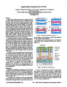
Figure 2.2: Merit criterion versus number of cells for three different access protocols (adapted from [33]). The plot shows that when the number of cells in the sending chip is low (smaller than 105 ), the ALOHA access protocol offers the best performance. When the number of cells is high (greater than 105 ), the probability of collisions increases. An increased number of collisions dramatically affects the performance of the ALOHA access protocol, reducing its throughput and increasing its latency. In this case the arbitrated access protocol is shown to be the most efficient.

access modality is certainly more efficient when the sending nodes are silent most of the time. Arbitrated access is preferable to ALOHA and priority encoder algorithms, if the timing skew introduced is negligible and loss of data cannot be tolerated by the system. For large numbers of sending nodes, arbitrated access shows the best performances. Typical numbers of sending nodes in the most recent neuromorphic implementations range from hundreds, to hundreds of thousands of nodes, arranged in one or two dimensional arrays, encouraging the choice of arbitrated AER. Arbitrated circuitry has a large overhead in terms of circuit and layout design, compared with non–arbitrated schemes. But as standard CMOS technology improves and we begin to design arrays with large number of neurons, the proportion of the arbiter layout with respect to the rest of the system becomes smaller and smaller. For example, in a 0.35 µm chip with 256 neurons and ≈ 10000 synapses, the core of the chip occupies an area of 6.8 mm2 whereas the arbiter layout area is 0.4 mm2 (about 6% of the core area).

2.3

Arbitrated AER for Multi–chip Systems

The AER protocol originally proposed by Mahowald [84] is for single sender, single receiver systems. This is known as the Point–to–Point (P2P) AER protocol [1]. The process

2.3. Arbitrated AER for Multi–chip Systems

13

Initiation Request Data Data Valid Acknowledge Figure 2.3: Point–to–Point handshake protocol. A node within the sender chip initiates a handshake cycle by prompting the sender to make a request (initiation signal). After making a request, the sender puts the data on the address event bus. Since the address lines may take different amounts of time to stabilize a data valid line is used to signal when the data on the address bus are set. The receiver acknowledges receipt of the data and the initiation signal is reset to let the sender drop the request and complete the handshake cycle.

\Initiation \Request \Acknowledge Data Figure 2.4: SCX handshake protocol. A node within the sender chip initiates a handshake cycle by prompting the sender to make a request. The sender can write the data on the AE bus only after the receiver acknowledges. The handshake cycle is complete only when both request and acknowledge are reset.

of sending events from one chip to the other is regulated by a handshake (see Fig. 2.3). A simple handshake involves two chips: a sender chip and a receiver chip. A node in the sender chip initiates an event by activating a request signal. The receiver chip must answer the request by activating an acknowledge signal, after which it reads the data on the address–event bus. After the acknowledge signal is activated, the sender chip removes the request to let the receiver chip removes the acknowledge signal. The handshake cycle is completed when the acknowledge signal is removed by the receiver chip, and another cycle can be initiated by a node in the sender chip. Systems containing more than two AER chips can be assembled using additional, off– chip arbitration. These off–chip arbiters can also use lookup–tables and processing elements to remap, time–stamp and perform digital operations on address–events [34, 37]. The P2P protocol is not suitable for multi–chip systems because the sender drives the address bus, shared by all senders in this case, as a consequence of activating the request. In a multi–chip system only the acknowledged sender should drive the address bus, to prevent data corruption in case two senders attempt to send an event at the same time. In 1998, Deiss et al. [37] proposed the SCX–1 Local Address–Event Bus (LAEB) for

14

Chapter 2. Address–Event Representation

multi–chip AER systems (SCX stands for Silicon Cortex, see section 2.4). The authors presented a communication protocol for multiple senders and multiple receivers on the same address bus. Each chip connected to the local address bus has a dedicated pair of request and acknowledge lines. The handshake protocol is represented in Fig. 2.4. A recent successful evolution of the AER is the burst–mode “word–serial” address– event link proposed by Boahen [16, 17, 18]. This design uses address–events to communicate between cells in the same or in different bidimensional arrays. Row and column addresses are not transmitted in parallel, as in previous designs, but serially. The loss in speed due to serial transmission is compensated by not retransmitting the row address if the next event is from the same row: row activity is encoded in a burst consisting of the row address followed by a column address for each active cell. Multi–chip systems can be build in a chain extending the single–transmitter-single–receiver link using merges and splits1 (see [30] for an example of such architecture).

2.4

AER Hardware Infrastructures

The hardware infrastructure is an essential instrument to fully characterize neuromorphic prototype chips. This infrastructure has to provide ways to stimulate and monitor the activity of a single chip. In addition, it has to be able to interface several chips and dynamically define the connectivity among them, implementing complex multi–chip systems. Furthermore, it should allow logging of data from all chips, allowing off–line analysis. Different approaches can be pursued to build neuromorphic multi–chip systems: dedicated full–custom circuits can be implemented to support specific AER devices, or a general–purpose full–custom architecture can be designed to host any AER device compliant to a certain standard. Several multi–chip systems have been implemented with both approaches. Examples of dedicated full–custom multi–chip systems are described in [30, 57]. These systems comprise EPROMs or FPGAs for remapping of the addresses, but they do not include any device to store the activity of the AER chips (requiring a separate acquisition instrument, usually a logic analyzer, to look at the system behavior) or to stimulate the chips with synthetic trains of spikes. More general architectures have been proposed [34, 37, 106] to interconnect, monitor and stimulate several AER devices. The first example of a general–purpose multi–sender multi–receiver communication framework for AER devices, called Silicon Cortex (SCX), is the one proposed in 1998 by Deiss et al. [37]. SCX is a fully–arbitrated AE infrastructure which can support up to six AER chips; larger systems can be assembled by linking together multiple boards. SCX provides a method of building a distributed network of local busses sufficient to build an indefinitely large system, co–ordinating the activity of multiple sender/receiver chips on a common bus. The user can configure arbitrary connections between neurons, set analog parameters and monitor the activity of the neurons. The most recent communication frameworks [34, 106] follow two different strategies. 1

The merge circuit combines the address events at its input with address events generated by the neuron array and sends them off chip via a transmitter. The split circuit makes two copies of the AER events appearing at its input.

2.5. The PCI–AER Hardware Infrastructure

15

In the context of the CAVIAR project2 , Serrano–Gotarredona et al. [106] proposed a distributed system in which a USB–AER board can be programmed to perform one of five different functions: (1) mapping of addresses, (2) capture of timestamped AEs, (3) reproduction of time–stamped sequences of AEs in real time, (4) transformation of sequence of frames into AEs in real time, (5) histogram AEs into sequences of frames in real time. Additional PCBs are used to record AE traffic on the AER bus; split one AER bus into 2, 3 or 4 busses; merge 2, 3 or 4 AER busses into a single bus; and capture time–stamped AEs to a computer. The hardware infrastructure described in this chapter, originally conceived and built by Vittorio Dante in Rome at the Physics Laboratory of the Italian Institute of Health [34], follows a different approach. It consists of a single full–custom general–purpose PCI board (the PCI–AER board) hosted in a workstation, that allows connection of up to four sender and four receiver chips, building a multi–chip system with arbitrary intra– and inter–chip connectivity, stimulating receiver chips with synthetic trains of spikes, monitoring and logging the activity of the sender devices. AER systems built using the PCI–AER board require a workstation in the loop and therefore are not as portable as the CAVIAR system, nevertheless these systems are more convenient for rapid prototyping tests, data analysis, and on–line reconfigurability. This board and its supporting software are the unique result of a team effort of several researchers from different institutions over several years. The Linux driver for the PCI– AER board was written by Adrian Whatley at INI. I contributed by writing library and test code for using the board, by debugging the setup, and by acting as the first beta–tester with a VLSI AER multi–neuron chip (described in chapter 5).

2.5 The PCI–AER Hardware Infrastructure 2.5.1 The PCI–AER Board The need for a custom device to easily interact with neuromorphic chips with spiking neural networks quickly increased with the emergence of the AER protocol as a standard for communication between these chips. In 2000, at the Physics Laboratory of the Italian Institute of Health (Rome, Italy) the PCI–AER project was started to provide flexible and easy interaction between a standard personal computer and an interconnected system of possibly heterogeneous AER chips. The PCI–AER board provides real–time routing between neuromorphic chips, with programmable connectivity, monitoring and stimulation of up to four chips and a communication bridge between AER and the PCI bus. The PCI-AER board takes the form of a 33MHz, 32-bit, 5V PCI bus add-in card (see Fig. 2.5) installed in a host personal computer. A 68-way cable is used to connect the PCI–AER board to a small header board (see Fig. 2.6) which can be conveniently located on the benchtop, and provides connectors for up to four AER receivers and four AER senders. The header board also electrically buffers the signals to and from the receivers and senders. Senders must use 2

CAVIAR is the acronym of the European funded project IST–2001–34124: Convolution AER Vision Architecture for Real Time.

FPGA 1

Monitor FIFO

PCI Interface

Mapper FIFO

SRAM

FPGA 2

Figure 2.5: PCI–AER board. The devices involved in the implementation of the three major functional blocks (see Fig. 2.7) are highlighted: MONITOR, MAPPER, and SEQUENCER FIFOs, FPGA1, and FPGA2. The SRAM is used to hold the mapper’s look–up table. A 68 pin cable connector is used to connect to the header board (see Fig. 2.6). The PCI interface manages the communication with the host personal computer through the PCI bus.

68 Pin Cable Connector

Sequencer FIFO

16 Chapter 2. Address–Event Representation

2.5. The PCI–AER Hardware Infrastructure From Sender Chips

Sequencer Connector

17

Cable Driver

68 Pin Cable Connector

To Receiver Chips Status LEDs

External Power Supply

Figure 2.6: PCI–AER header board. The header board is connected to the PCI–AER board through a 68-way cable and it can be conveniently located on the benchtop. The header board provides connectors for up to four AER receivers and four AER senders plus the SEQUENCER connector. The external board has five LEDs, three yellow and four red. Close to the 68 pin connector there is the Power ON LED. Next to it there are FIFO Full alert LEDs for the MAPPER, MONITOR and SEQUENCER respectively. The yellow LEDs are used to indicate the status (LED on means enabled) of the three functional blocks (SEQUENCER, MONITOR, and MAPPER respectively).

the SCX multi-sender AER protocol [36], in which request and acknowledge signals are active low, and the bus may only be driven while the acknowledge signal is active. Receivers may use either this SCX protocol, or they may choose to use a P2P protocol [1] in which request and acknowledge are active high and the bus is driven while request is active. Which protocol is generated by the board may be selected under software control. As illustrated in Fig. 2.7, the PCIAER board can perform three functions which are executed by blocks we refer to as the monitor, sequencer, and mapper. These blocks are controlled by two FPGAs (FPGA1 and FPGA2 in Fig. 2.5) on the board. The PCI–AER board has four main components: Arbiter Up to four sender chips can be connected to the PCI–AER board. The on board arbiter implements arbitration of events generated by the different sender chips. This allows multiple sender devices to access the AE bus. Monitor Arbitrated events generated by the sender chips are time–stamped and recorded by the monitor. Stored events can be then accessed from the personal computer via the PCI bus. This is useful for logging data, and it allows the user to analyze the activity of the connected devices off–line, without affecting the performance of the system. Sequencer Using the sequencer, up to four receiver chips can be stimulated with pre– defined spike trains. Synthetic spike trains can be generated using the personal computer and downloaded to the board via the PCI bus. Mapper The connectivity pattern between up to four sender chips and up to four receiver chips is implemented by the mapper. Transceiver chips can be connected as sender

18

Chapter 2. Address–Event Representation PCI-AER BOARD FPGA 1 TIMER 32 Bit Counter

8Kx18bit

PCI to Local Bus Interfac e

SEQUENCER

MAPPER-IN

ARBITER

Local Bus

PCI Bus

Async. FIFO

MONITOR

Arbiter Input MUX

8Kx18bit Async. FIFO

FPGA 2 MAPPER-OUT

AER DEMUX

Cable to Header Board

8Kx18bit Async. FIFO

SRAM 2M Word

Figure 2.7: Block diagram of the PCI–AER interface board showing its three major functional blocks, i.e. the MONITOR, the SEQUENCER, and the MAPPER (divided into MAPPER–IN and MAPPER–OUT). These (and other blocks) are implemented in two FPGAs on the PCI–AER board. Also shown are the FIFOs, the interface to the PCI bus, the SRAM used to hold the mapper’s look– up table, the cable buffers, and the interconnecting buses.

and receiver at the same time, using the PCI–AER to externally configure their “internal” connectivity. Arbitrary network topologies can therefore be implemented and reprogrammed on–line. Using these components the board implements the functions described below. Monitoring The PCI–AER board can monitor the spiking activity of up to four sender chips. The monitor captures and timestamps events coming from the attached AER senders via an arbiter, and makes those events available to the personal computer for further processing. A timer is implemented in one of the FPGAs, and when an incoming address–event is read, a timestamp is stored along with the address in an 8KWord First–In First–Out (FIFO) memory. This FIFO decouples the management of the incoming address–events from read operations on the PCI bus, the bandwidth of which must be shared with other peripherals in the personal computer such as the network card. Interrupts to the host personal computer can be generated when the FIFO becomes half–full and/or full, and in the ideal case, the driver will read time stamped address–events from the monitor FIFO whenever the host

2.5. The PCI–AER Hardware Infrastructure

19

CPU receives a FIFO half–full interrupt at a rate sufficient that the FIFO never fills or overruns, given the rate of incoming address–events. Each event is stored in the form of three successive 18 bits words. The two most significant bits of the word encode the type of information stored in the other 16 bits. A word can contain four different type of information: AE, Time High (16 most significant bits of the 32 bits word encoding the time–stamp), Time Low (16 less significant bits of the 32 bits word encoding the time– stamp), Error or Control code. The time resolution can be set to four different values: 1, 10, 50 or 100 µs. The AE is coded differently depending on the number of sender chips: 1 sender chip 16 bit address word. 2 sender chips The most significant bit of the AER address encodes the chip label. The address word is encoded by the remaining 15 less significant bits. 4 sender chips The two most significant bits of the AER address encode the chip label. The address word is encoded by the remaining 14 less significant bits. Stimulating The PCI–AER board can be used to stimulate receiver chips using synthetic trains of AEs. This function is implemented by the sequencer. These events may for example represent a pre–computed buffered stimulus pattern, but they might also be the result of a real time computation. This allows, for instance, software simulations of VLSI devices to provide input to real VLSI hardware while the former VLSI devices are still under development. As soon as the real device is available, the software simulation can be seamlessly replaced. Like the monitor, the sequencer is decoupled from the PCI bus using an 8KWord FIFO. The host writes an interleaved sequence of words representing addresses and time delays to the sequencer FIFO. The sequencer then reads these words one at a time from the FIFO and either emits an address–event or waits the indicated number of microseconds. The events generated can be transmitted on any of the four output channels. Mapping Events coming from sender chips can be mapped to receiver chips using the PCI–AER board. The use of a transceiver chip combined with this function allows programmable connectivity between neurons on the same chip. Different chips can also be interfaced by defining a connection table among their neurons. The mapper can operate in three different modes: Pass–through The input address events are simply replicated on the output. One–to–one The input address events are used as pointers to a look–up table stored in the mapper SRAM. The retrieved content of the table for each input address is the target address on the output.

20

Chapter 2. Address–Event Representation One–to–many Each input address event generate multiple output events to different targets. The input address is used as a pointer to the first memory location (in the mapper SRAM) of a list of targets.

The mapper has a FIFO which decouples the asynchronous reception of the incoming address events from the generation of outgoing address events. Once configured and after the look–up table has been filled with the required mappings, the mapper operates entirely independent of the host personal computer. All of the necessary operations, including table look–up, are performed by one of the FPGAs on the PCI–AER board.

2.5.2

Supporting Software

Low level control of the PCI–AER board is carried out by a Linux software driver which allows the operating system to access and modify the status of the board. The driver supports up to four PCI–AER boards in one machine. The logically separate functions of the Mapper, Monitor and Sequencer are supported by three minor devices for each board. The separation of Mapper, Monitor, and Sequencer has the advantage of giving the desired degree of granularity of control over simultaneous use policy (not more than one process may open each minor device, but separate processes may be used for reading, writing and mapping control). The Linux driver for the PCI–AER board was developed by Adrian M. Whatley at the Institute of Neuroinformatics (University and ETH Zurich). A user of the hardware infrastructure should not need to understand and use the driver interface to be able to test neuromorphic chips. Instead of accessing a particular configuration register to set the appropriate value for using a defined functionality of the board, the user should be able to simply use the desired functionality through more high level software functions. For this purpose a library of C functions was implemented. The PCI–AER library is a set of low/intermediate level functions useful for accessing and controlling the PCI–AER board. They can be used in spike train generation code, in data–logging code and in other programs that need to access the PCIAER board. Specifically, library calls allow the user to easily perform all operations supported by the PCI–AER board and driver. For example, the following sequence of operations can be executed to read and store the activity of all senders connected to the PCI–AER board: 1. Open Monitor. 2. Read n AEs (where n is an arbitrary number). 3. Close Monitor. These high level commands open the driver and call a set of low level routines to perform the required operation. Many other high level commands are included in the library and App. B contains a detailed description of all library calls. I initially developed most of these commands under the supervision of Adrian Whatley and participated in the debugging of the library. The code has been further debugged and enhanced by Adrian Whatley and other collegues.

2.5. The PCI–AER Hardware Infrastructure

21

All the software is implemented in C language and can be easily used with a Matlab interface to develop an user–friendly access system to the chips through the PCI–AER board.

Chapter 3

Analog Circuits for Implementing Spike Based Processing Models Neuromorphic engineering makes use of analog very–large–scale–integrated (VLSI) circuits to implement biologically–inspired processing systems. Analog circuits perform massively parallel real–time computation with many orders of magnitude less power than general–purpose computers. In this Chapter, I will introduce some basic analog circuits necessary for understanding the neuromorphic circuits I used as building blocks in my system. I start with a quick review of the Metal–Oxide–Semiconductor Field Effect Transistor (MOSFET) device [81, 88], move on to two transistor circuits that are basic blocks for the silicon synapses, describe the transconductance amplifier used in the silicon neuron, the neuron circuit itself and an adaptive synapse circuit, able to model short–term depression and facilitation effects. Since almost all the neuromorphic circuits I used in my system are operated in the subthreshold regime, in the next section I will discuss the MOSFET device and the analog circuits always referring to this regime.

3.1 Subthreshold MOSFET Characteristic The MOSFET is composed of a Metal–Oxide–Semiconductor (MOS) structure (gate) and two diffusions (drain and source). A schematic drawing of the structure of an n–type MOS transistor is shown in Fig. 3.1. The substrate is p–type (holes are the majority carriers). The drain and source diffusions are heavily doped n–type (electrons are the majority carriers). The channel is the region underneath the gate and between the drain and source diffusions. The charge in the channel is carried by electrons. The p–type MOS has an n–type channel where the charge is carried by holes supplied from the p–type source and drain regions.

23

24

Chapter 3. Building Blocks SiO2

Polysilicon gate drain

source

L

W

n+ n+

p

Figure 3.1: Schematic drawing of the physical structure of an n–type MOS transistor. Two n+ diffusions in the p substrate implement the drain and source regions. The gate is implemented by a polysilicon layer isolated from the channel by a SiO2 layer.

In a CMOS process, the n–FETs and p–FETs are fabricated on the same substrate. In the process I used, n–FETs are implemented in the common p− substrate and p–FETs in an n–well within the substrate. The MOS transistor has four terminals (MOSFET symbols for both n and p–type transistors are shown in Fig. 3.2): the source (S), the drain (D), the gate (G) and the bulk (B). The expression for the current that flows between drain and source is ³ qVs ´ qVg qVd Ids = I0 e KT e− KT − e− KT (3.1) where

W L is the dark or leak current. In the derivation of the Ids current, the Early effect and the fact that only part of the voltage applied to the gate is present on the channel are neglected [81]. Taking into account these two effects and using Vds for Vd − Vs , we can write: µ ¶ qκVg Vds Vs Vds −q KT −q KT KT Ids = I0 e e + 1−e (3.2) Ve Φ0

I0 = qDN0 e−q KT

where κ is the capacitive coupling ratio from gate to channel [81] and Ve is the Early voltage. Typical values for κ are between 0.5 and 0.9, while Ve varies from 20 V to 750 V depending on the transistor’s length L.

3.2. Differential Pair and Transconductance Amplifier S

S

S

B

G

25

B

G

D

B

G

D

D

S

S

(a) S

B

G

B

G

D

D

D

B

G

(b)

Figure 3.2: Symbols for (a) an n–type MOS transistor and (b) a p–type MOS transistor. The bulk terminal can be omitted when connected to ground for n–type MOS and to the power supply for p–type MOS. Throughout the rest of this thesis we will use the symbols in the rightmost column.

Two regions of operation can be distinguished depending on the value of the drain–to– source voltage: the linear (or ohmic) region and the saturation region (see Fig. 3.3). For a given gate voltage Vg , in the linear region the current increases linearly with Vds , while in the saturation region the current is independent of Vds (if the Early effect is negligible). When Vds is small (linear or triode region) a linear function is obtained from the Taylor’s series expansion of Eq. 3.1: Ids = I0 eq

κVg −Vs KT

q Vds KT

For Vds > 4KT /q (saturation region) the exponential in Eq. 3.2 is much smaller than one and so can be neglected and, again neglecting the Early effect, the current is approximately given by κVg −Vs Ids = I0 eq KT . (3.3)

3.2 Differential Pair and Transconductance Amplifier The transconductance amplifier, used in the I&F neuron (see section 3.8) is a device that generates an output current which is a function of the difference between its two input voltages. It is composed of two basic circuits: the differential pair and the current mirror

26

Chapter 3. Building Blocks V =0.55 gs

500

Vgs=0.53 Vgs=0.51

400

V =0.49

Ids (nA)

gs

Vgs=0.47

300

Vgs=0.45

200

100

0 0

0.2

0.4

0.6

0.8

1

Vds (V) Figure 3.3: The current Ids as a function of Vds , for Vgs between 0.45 V and 0.55 V , as measured from a Spice simulation. The current is linear for small values of Vds (ohmic or linear region) and is approximately constant for Vds > 4UT (saturation region). The slight increase of Ids for increasing values of Vds in the saturation region is due to the Early effect.

(see section 3.4). A schematic circuit of the differential pair is shown in Fig. 3.4. The MOSFET Mb acts as a voltage controlled current source. The current, Ib , is set by the bias voltage, Vb . The sharing of this current between M1 and M2 depends on the difference between the two input voltages, V1 and V2 . Assuming that all transistors are operated in the subthreshold saturation domain and have the same subthreshold slope factor κ, we can compute I1 and I2 as a function of the bias current and the input voltages. We can use the I–V relationship in the saturation region (Eq. 3.3) for transistors M1 and M2 : κV1 − UV T

(3.4)

κV2 − UV UT T

(3.5)

I1 = I0 e UT I2 = I0 e The bias current is the sum of I1 and I2 :

− UV

Ib = I1 + I2 = I0 e

T

³ e

κV1 UT

+e

κV2 UT

´

Solving for V we obtain:

Ib 1 κV1 2 I0 e UT + e κV UT Combining this equation with Eq. 3.4 and 3.5 yields − UV

e

=

T

κV1

I1 = Ib

e UT e

κV1 UT

+e

κV2 UT

= Ib

1 1+e

κV2

I2 = Ib

e UT e

κV1 UT

+e

κV2 UT

= Ib

κ UT

(V2 −V1 )

1 − Uκ (V2 −V1 )

1+e

T

3.2. Differential Pair and Transconductance Amplifier

V1

I1

I2

M1

M2

V

27

V2

Ib Vb

Mb

Figure 3.4: Schematic diagram of the differential pair. The voltage bias Vb sets the total current Ib (bias current) that can flow in the circuit. The bias current flows in one of the two branches depending on the difference between the two input voltages V1 and V2 . When one bias voltage is greater than the other (and the difference between them is at least in the order of a few Ut /κ) the current flows only in its branch.

M4 Iout

M3

V1

I1

I2

M1

M2 Ib

Vb

Mb

Vout

V2

− Vout

V2

V1

+ Vb (b)

(a) Figure 3.5: (a) Schematic diagram of the transconductance amplifier. The transconductance amplifier is composed of a differential pair (see Fig. 3.4) and a current mirror (see Fig. 3.7). The current mirror is used to subtract the two output currents of the differential pair. (b) Symbol of the transconductance amplifier. The symbol provides a compact representation of the transconductance amplifier to be used in complex circuits. The terminal for the bias voltage Vb is often omitted.

28

Chapter 3. Building Blocks

V=V0 C1

V

C2 A

C1

C2

A + − ∆V

(b)

(a)

Figure 3.6: Capacitive voltage divider. (a) Initially capacitors C1 and C2 are in parallel and a voltage V0 is present on their common node. (b) When a voltage ∆V is applied on node A the C2 voltage on the common node is changed by ∆V C1+C2 .

If V1 − V2 is greater than zero and of the order of a few UT /κ, then I1 ∼ Ib and I2 ∼ 0. If V1 − V2 is smaller than zero and of the order of a few UT /κ, then I1 ∼ 0 and I2 ∼ Ib . To implement the transconductance amplifier, a current mirror is used to subtract the two output currents of the differential pair (see Fig. 3.5). As long as all the MOSFETs stay in saturation and the bias current is in the subthreshold regime, the output current of the transconductance amplifier is given by Iout = I1 − I2 = Ib

κV1

κV2

κV1 UT

κV2 UT

e UT − e UT e

+e

= Ib tanh

κ(V1 − V2 ) 2UT

The transconductance amplifier is often used as a comparator in the open loop configuration. The output voltage is high when V1 > V2 , and it is low when V1 < V2 [81]. This property is used in the implementation of the I&F neuron (see section 3.8) to compare the membrane voltage with the threshold for spike emission.

3.3

Capacitive Voltage Divider

The capacitive voltage divider, composed of two capacitors, is used in the I&F neuron circuit to implement a positive feed–back involved in the generation of the output pulse. In this context, the relevant behavior is the response to an abrupt change in the voltage on one node of one capacitor (see node A in Fig. 3.6). Initially (see Fig. 3.6(a)) the two capacitors are connected in parallel and the voltage, V , on their common node is equal to V0 . If Q is the total charge stored on the two capacitors, we can write: Q = V0 (C1 + C2) A sudden change in the voltage on node A produces a change in the voltage, V , on the common node. This change can be computed by applying the principle of charge conservation to the charge stored into the two capacitors before and after the sudden change in voltage: V0 (C1 + C2) = V C1 + (V − ∆V )C2

3.4. Current Mirror

29

Iin

M1

Iout

Vg

M2

M1

Vg

Iout

Iin (a)

M2

(b)

Figure 3.7: Current mirror. The current mirror is used to replicate currents. The replicated current has the opposite sign of the original current, and can be an amplified or reduced version of it. (a) Schematic diagram of the n–type current mirror. (b) Schematic diagram of the p–type current mirror.

We can then write the following expression for the voltage: V = V0 + ∆V

C2 C1 + C2

(3.6)

When a voltage, ∆V , is applied between the ground rail and capacitor C2 the voltage on C2 the common node is changed by ∆V C1+C2 .

3.4 Current Mirror The current mirror is a simple circuit used to replicate, amplify and reduce the amplitude of currents. Several output currents can be generated from a single input current. The output of the current mirror replicates the input current, multiplied by a factor that is function of the transistors’ geometry. The schematic diagrams of an n–type and a p–type current mirror are shown in Fig. 3.7. The MOSFET M1 is called master because the reference current flows through it; the MOSFET M2 is called slave because it generates the replicated current. The master transistor is a diode–connected MOSFET (Vgd = 0; the transistor is operated in saturation). The input current univocally determines the gate voltage of the master transistor. If the slave transistor is geometrically identical to the master transistor, and as long as the slave is operated in saturation, the output current is equal to the input current. In the most general case, the parameters related to the technology are identical for the two transistors but their geometry is different. For subthreshold input currents we can write µ² W1 κVg /UT e tox L1 µ² W2 κVg /UT e = tox L2

Iin = Iout

30

Chapter 3. Building Blocks

Vτ IC

Iin

C Iout

ID

Vin Iout

ID IC

Vin

Iin

C

Vτ (a)

(b)

Figure 3.8: Current Mirror Integrator (CMI). The CMI, composed of two transistors in the current mirror configuration (see Fig. 3.7) and one capacitor, implements a non–linear integration of its input current. (a) Schematic diagram of the n–type CMI. (b) Schematic diagram of the p–type CMI.

where µ is the electrons or holes mobility, ² is the permittivity and tox is the thickness of the oxide. The output current is then given by Iout =

3.5

W2 L1 Iin W1 L2

Current Mirror Integrator

The Current Mirror Integrator (CMI) is a non–linear integrator often used to implement silicon synapses for spiking neural networks [20, 53, 62, 100]. This circuit is composed of two transistors and one capacitor (see Fig. 3.8). Assuming that all transistors are in the subthreshold saturation region, we have: n–type CMI Iout (t) ID (t)

p–type CMI

Vτ

= e UT = A

(t) IC (t) = C dVin = dt

= Iin (t) − ID (t) Vin (t) =

UT κ

(t) ln Iout In0

Iout (t) ID (t)

=e

Vτ −Vdd UT

=A

IC (t) = C dtd (Vdd − Vin (t)) = = Iin (t) − ID (t) Vdd − Vin (t) =

UT κ

(t) ln Iout Ip0

where κ is the subthreshold slope factor and UT is the thermal voltage. Combining the

3.5. Current Mirror Integrator

31

three equations above, we obtain the dynamics of the output current (Iout ) for the CMI circuit (valid for n and p–type circuits): µ ¶ dIout (t) κ Iout (t) Iout (t) Iin (t) − (3.7) = dt CUT A Solving this first order differential equation separately for Iin (t) = Iin0 and Iin (t) = 0, we can obtain the response to a current pulse: Iin (t) = Iin0 u˙ (t − t0 ) where u(t) is a step function and t0 represents the onset of the step. For Iin (t) = Iin0 , the output current can be expressed as follows: ³ ³ ´´  Iin −Iout (0) κIin Iin 1  tanh t − ln + I2in f orIin > Iout (0)  CUT 2 Iout (0)  2 Iout (t) = ³ ³ ´´    Iin coth κIin t − 1 ln Iout (0)−Iin + I2in f orIin < Iout (0) 2 CUT 2 Iout (0) When Iin (t) = 0, the output current is given by Iout (0) κ I (0)t CUT out

Iout (t) =

+1

The output current increases proportional to a hyperbolic tangent when the step is applied, and decreases proportional to 1/t after it is removed.

3.5.1 Response to Spike Trains: Approximate Solution We are interested in the response of the CMI to a spike train, which is the typical input for a synapse. In his PhD thesis, Boahen [14] proposed the following approximate analytical solution for the response of a CMI to a spike train. Rewriting Eq. 3.7 as follows we can obtain an approximate solution for the output current Iout (t): QT d(1/Iout (t)) 1 1 = − Iin (t) dt AIin (t) Iout (t) where QT = CUT /κ. In the most general case, we can write the solution of this first order differential equation in the form of the integral equation: Iout (t) =

Z Iout (t0 ) AQT

Iout (t0 ) t

− Q1

e

T

Ru t

Iin (s)ds

du + e

Rt

− Q1

t0

T

Iin (u)du

t0

where t0 is the onset time of the first input pulse. For a sequence of instantaneous current pulses at the input, the general solution reduces to Iout (t) = Iout (t0 AQT

à n X ) j=1

Iout (t0 ) − Q1

e

T

Pn

i=j qi

!

(tj − tj−1 ) + (t − tn )

− Q1

+e

T

Pn

i=1 qi

32

Chapter 3. Building Blocks

for tn ≤ t < tn+1 , where ti = t0 , t1 , t2 , ... (with t0 < t1 < t2 < ...) are the times at which the pulses occur and {qi } are the amounts of charge that each spike supplies. When the dynamics reach the steady–state each input spike adds the same amount of charge qα on the capacitance. The current flowing through the output transistor (in saturation) is Iout = In0 exp (κVin /UT ). If a charge qα is stored into the capacitor, there is a change in the input voltage given by ∆Vin = qα /C. The output current is then given by κ

0 Iout = In0 e

Vin +∆Vin UT

qα κ CU

= Iout e

T

qα

= Iout e QT .

We define 1 + α ≡ exp (qα /QT ) as the factor by which the output current is multiplied by each input spike. In this case we obtain: Iout (t) =

Iout (t0 ) Ã n ! X Iout (t0 ) (1 + α)j−(n+1) (tj − tj−1 ) + (t − tn ) + (1 + α)−n AQT j=1

We can break this equation into two parts: Iout (t) =

Iout (t+ n) Iout (t+ n) (t AQT

− tn ) + 1

, tn ≤ t < tn+1 Iout (t0 )

Iout (t+ n) = Iout (t0 ) AQT

n X

(3.8) (3.9)

(1 + α)j−(n+1) (tj − tj−1 ) + (1 + α)−n

j=1

Where t+ n is the instant immediately after the time of the input spike (tn ). If the inter–spike intervals are all the same (T ≡ tj − tj−1 , j = 1, 2, ...) we can sum the geometric series in the denominator of Eq. 3.9 and obtain Iout (t) =

Iout (t+ 0 + nT ) Iout (t+ 0 +nT ) (t AQT

Iout (t+ 0 + nT ) =

1 IˆT

−

+ , t+ 0 + nT ≤ t < t0 + (n + 1)T

(t+ 0

+ nT )) + 1 1 ³ ´ , n = 1, 2, ... + Iout1(t0 ) − Iˆ1 (1 + α)−n T

AQT IˆT ≡ α T In the steady–state we can consider (1 + α)−n ¿ 1, and the current immediately after each spike converges to IˆT . The time taken to reach this equilibrium depends only on the number of spikes, and scales proportionally to the frequency of the input train. This analysis demonstrates how the circuit integrates regular trains of spikes and reaches a steady state which is function of the input (α and T ), the circuit geometry (QT ) and its biasing (A). When the stimulation finishes, the output current decays approximately as 1/t (see Eq. 3.9). This approximate solution assumes that the input pulses are instantaneous, and does not take into account the dependence of α on the circuit and input signal parameters.

3.5. Current Mirror Integrator

33

3.5.2 Response to Spike Trains: General Analytical Solution Another strategy to obtain an exact and more general expression of the CMI’s response is to study the dynamics of the input voltage, Vin , in response to the applied pulses. The output current can be derived from Vin using the equation for the transistor subthreshold saturation region (Iout = In0 exp (κVin /UT )). Furthermore, to compute a steady state solution, we examine the case in which the spike duration (∆t) and the interval between spikes (T) are constant. The dynamics of Vin is described by the following equation: C

dVin (t) In0 κVUin (t) = Iin (t) − e T dt A

(3.10)

where    Iin (t) = Iin f or ti < t < ti + ∆t  

Iin (t) = 0

f or ti + ∆t < t < ti + ∆t + T = ti+1

and ti ≡ t0 < t1 < t2 ... are the times at which the pulses occur. Solving Eq. 3.10 separately for the two conditions mentioned above, we obtain: · µ ¶ ¸  Iin κVin (ti ) − (t−t ) − i U I I   Vin (t) = − κT ln e QT e UT − AIn0in + AIn0in    (3.11) · ¸   κV (t +∆t)  − inU i  In0 T  Vin (t) = − UκT ln AQ (t − t − ∆t) + e i T where QT = CUT /κ, and the two equations are valid for ti < t < ti + ∆t and ti + ∆t < t < ti+1 respectively. Using these equations it is possible to show that ¶ µ ¶µ I A 1 − Qin ∆t T T < QT − 1−e In0 Iin is the necessary condition to accumulate charge on the capacitor. The output current is simply derived from Eq. 3.11, as mentioned above:   ; ti < t ≤ ti + ∆t Iout (t) = − Iin (t−t ) “ 1  ”  i  1 1 1 e QT + −  Iout (ti ) AIin AIin      Iout (t) =

1 AQT

1 (t−ti −∆t)+ I

1 out (ti +∆t)

;

ti + ∆t < t ≤ ti+1

34

Chapter 3. Building Blocks

Steady State At the steady state, Vin (ti ) = Vin (ti+1 ), Vin (ti + ∆t) = Vin (ti+1 + ∆t) ∀i and the input voltage, Vin , oscillates between the two values     I in  − ∆t     1−e QT !  Vin (ti ) = UκT ln  I  − in ∆t  I I n0 T + n0  1−e QT  AQT AIin             Vin (ti + ∆t) = − UκT ln     AQ

T

 In0 T

!

Iin ∆t e QT −1

+

In0  AIin 

The output current then oscillates between the two values   Iout (ti ) = 0 T A 1+ 1    I Iin  − in ∆t C  B QT @1−e QT  A  Iout (ti + ∆t) =      

A

T 1+ 1 Iin Iin B QT ∆t C QT @e −1A 0

The steady–state current increases with decreasing interval T between two consecutive spikes of the input train, increasing A, increasing amplitude of the input current Iin and increasing pulse width ∆t (as already shown in the approximate solution).

3.6

Excitatory and Inhibitory Synapses

Excitatory and inhibitory synapses can be easily implemented using p–type and n–type CMI (see section 3.5) respectively. To be able to stimulate these synapses using the AER protocol, we need a few more transistors. A circuit diagram of a complete excitatory synapse, including AER interfacing circuits, is shown in Fig. 3.9. Since we are interested in implementing two–dimensional arrays of silicon synapses, the circuit can be selected by a row and a column signal (VQy and VQx ). Transistors M 1 and M 2 in Fig. 3.9 act as digital switches, and the current set by the bias voltage, Vw , on transistor M 3 flows only when both the row and column signals, VQy and VQx , are high. Transistors M 4 and M 5 and the capacitor C implement the current mirror integrator, as described in section 3.5. Transistor M 6 is a cascode transistor controlled by the bias voltage Vcasp , used to isolate the output of the synapse from the voltage changes occurring at the membrane voltage of the post–synaptic neuron.

3.7

The Adaptive Synapse

Silicon synapses are circuits, typically used in VLSI networks of I&F neurons [14, 28, 41, 66], that implement models of biological synapses. Recent developments in the neuroscience community show that biological synapses are not simple interfacing elements

3.7. The Adaptive Synapse

35

Vτ C M4

M5 Vcas

Vw

M3

VQy

M2

VQx

M1

M6 Iout

Figure 3.9: Schematic diagram of the excitatory synapse. Transistors M 4 and M 5, and capacitor C , implement a p–type CMI (see Fig. 3.8). The input current of the CMI is set by the bias voltage Vw , and can flow only when the synaptic circuit is stimulated (both VQx and VQy are high). Transistors to prevent pump charge effect by transistor M 1 and M 2 (see Fig. 3.10) are omitted in the drawing, but included in the implemented circuit.

Vτf

Vpu

Cf M4

M5 If Vcasp

Vwf

M3

VQy

M2

VQx

M1

M7

M8 M10

M9 Vpix_ack Vwd

M11

M6

Iout

Vcasn

M13 Id

M12

M14 Cd

Vτd Figure 3.10: Schematic diagram of the adaptive synapse. Transistors M 4–M 5, and capacitor Cf implement the facilitating CMI of the synaptic circuit. Transistors M 12 and M 14, and capacitor Cd , implement the depressing block. Transistors M 7–M 8 prevent pump charge effects [20] by transistors M 1 and M 2. When the synapse is stimulated (both VQx and VQy are high), the facilitating CMI integrates the current set by the bias voltage Vwf , and the depressing CMI integrates the current set by the bias voltage Vwd .

36

Chapter 3. Building Blocks

for transmitting signals between neurons, but play an important computational role in biological neural networks [83]. One of the peculiar properties of biological synapses is their ability to exhibit short-term plasticity: the dynamic modulation of synaptic strength by the timing of the input stimulation [123]. Although there has been significant progress in understanding the mechanisms underlying short-term synaptic plasticity, its functional relevance in neural circuits remains relatively obscure. Several hypotheses have been proposed for the computational role of short-term synaptic plasticity [122], including local gain control [2], stimulus specific adaptation [25], and nonlinear temporal summation [26]. Practical constraints on computational resources restrict the testing of these hypotheses to relatively small simulated networks, simple input signals, or long simulation times. Silicon implementations of synapses that exhibit short–term plasticity are suitable for evaluating the computational roles of synaptic adaptation in large networks of spiking neurons, using complex stimuli and in real-time [100]. I propose an analog circuit for implementing such a type of synapse. The core of the adaptive synaptic circuit consists of two CMIs [14, 61] (see section 3.5), which integrate the input spikes and produce a positive (facilitating) and a negative (depressing) current with different dynamics. Each time an input spike arrives, the facilitating CMI adds a set amount of charge onto its integrating capacitor, modifying the facilitating current accordingly. At the same time, a different amount of charge is summed onto the capacitor of the depressing CMI, modifying the depressing current. The positive facilitating and negative depressing current are then summed to generate the net output current. The proposed AER synaptic circuit is shown in Fig. 3.10. The facilitating CMI is implemented by transistors M 4–M 5 and by capacitor Cf . The depressing CMI is implemented by M 12 and M 14 and by Cd . Both CMIs are connected to circuit blocks that implement the AER interface (transistors M 1–M 2 and M 9-M 10, all acting as digital switches). The AER part of the synaptic circuit operates as follows: upon the arrival of a request signal, the row and column encoders set the voltages VQy and VQx of the synapse identified by the row and column addresses high (see Fig. 3.13). Transistor M 9 then generates the AER acknowledge signal transmitted back to the sender device. When the synapse is addressed, transistors M 1–M 2 and M 10 are active and the currents set by the bias voltages V wf and V wd flow through transistors M 3 and M 11 respectively. The capacitors Cf and Cd integrate these currents, changing the voltages across them. The bias voltages V τf and V τd are used to change the temporal dynamics of the facilitating and the depressing parts of the synapse. The facilitating current, If , has an exponential dependence on the voltage across capacitor Cf and on the voltage V τf ; similarly, the depressing current, Id , changes exponentially with the voltage across capacitor Cd and with V τd . The synaptic output current, Iout , is the sum of the output currents of the two CMIs (when they are not limited by the cascode transistors M 6 and M 13). To derive the dynamics of Iout in response to a train of spikes, we need to evaluate the response of the two CMIs. If we consider an input train of spikes with fixed duration (∆t) for which ti = t0 , t1 , t2 , ... (with t0 < t1 < t2 < ...) are the times at which the pulses occur, the volt-

3.7. The Adaptive Synapse

37

1.4 1.2

Voltage (V)

1 0.8 0.6 0.4 V(Cf) (V) V(Cd) (V)

0.2 0 0

0.05

0.1 0.15 Time (s)

0.2

0.25

Figure 3.11: Voltages across the facilitating capacitor Cf and the depressing capacitor Cd in response to a 50 Hz spike train (analytical derivation). The facilitating CMI is set to reach the steady– state after the first input spike. The depressing CMI is set to reach the steady–state after several input spikes (5 in this example). The different time constants of the two CMIs produce the total output current shown in Fig. 3.12.

0.16 0.14 0.12

Iout (µ A)

0.1 0.08 0.06 0.04 0.02 0 −0.02 0

0.05

0.1 0.15 Time (s)

0.2

0.25

Figure 3.12: Output current of the adaptive synapse in response to a 50 Hz spike train (plot of the analytical expression of the current) produced by the dynamics of the facilitating and depressing CMIs shown in Fig. 3.11. The output current is mainly due to the facilitating CMI for the first few spikes. The depressing current slowly increase until it has an effect on the output current and produces an adaptive total response.

38

Chapter 3. Building Blocks

age across the capacitor Cf is given by (see section 3.5) · Iw µ κV (C )(t ) ¶ ¸ i f UT I0 I0 − Q f (t−ti ) − U T V (Cf )(t) = − ln e T e − + κ AIin AIwf · ¸ κV (Cf )(ti +∆t) UT I0 − UT V (Cf )(t) = − ln (t − ti − ∆t) + e κ AQT

(3.12) (3.13)

where QT = CUT /κ and Iwf is the current set by the bias voltage V wf . Equation 3.12 holds during the spike (ti < t ≤ ti + ∆t), and Eq. 3.13 holds between two spikes (ti + ∆t < t ≤ ti+1 ). If the interval between spikes is constant and equal to T, a steady state is reached and the voltage oscillates between two values. Analogous equations can be written for the voltage across the capacitor Cd . Figure 3.11 shows these voltages in response to a 50 Hz spike train for typical values of the parameters in Eqns. 3.12 and 3.13. The depressing part of the circuit is set to be slower than the facilitating one, to produce a negative current that slowly “depresses” the output of the synaptic circuit, implementing a synapse that exhibits short–term depression. Between spikes the voltage across the depressing capacitor, Cd , can be bigger than the voltage across the facilitating capacitor, Cf , leading to a negative output current. To prevent this, I added a transistor acting as a digital switch to block the negative current when the input spike is not active. The equations for the facilitating and depressing current can be derived using the expression for the voltages across the capacitors Cf and Cd respectively and the drain–source current for the transistor subthreshold saturation region (Ids = I0 exp (κVgs /UT )). The resulting output current, Iout = If −Id , is plotted in Fig. 3.12 (the depressing part of the current Id was set to zero whenever the input spike is not active).

3.7.1

Experimental Results

To characterize the response properties of the synaptic circuit, I fabricated a prototype chip using a standard 1.5µm CMOS technology. The chip (see Fig. 3.13) implements an AER transceiver neural network, and comprises several instances of the circuit shown in Fig. 3.10, leaky integrate–and–fire neurons of the type described in [62] (see section 3.8) and AER interfacing circuits. The response of the synaptic circuit was tested by stimulating it with periodic trains of pulses at different frequencies, and by measuring the change in the voltage across the input capacitor of the leaky integrate–and–fire neuron connected to it. In biology this change is commonly referred to as an excitatory post synaptic potential (EPSP). The EPSP was measured using the Cursor function of a Tektronix oscilloscope model TDS 420A. This function allows two cursors to be placed on the acquired trace, and to measure the distance between them. Placing the cursors at the lower and upper end of the EPSP gives us a measure of the EPSP amplitude in voltage. The measurement error associated with each cursor is half of the minimum step of the cursor itself, which depend on the selected voltage scale. The total measurement error is then given by the amplitude of the minimum step allowed to the cursor. The four voltages V wf , V τf , V wd and V τd (see Fig. 3.10) are used to shape the EPSP

3.7. The Adaptive Synapse

39

Column address AER input request signal

R o w a d d r e s s

R o w e n c o d e r

Column encoder

S

S

S

S

S

S

S

S

S

S

S

S

S

S

S

S

S

S

T o

S

S

S

S

S

S

SOMA

SOMA

SOMA

A E R o u t p u t c i r c u i t s

Figure 3.13: Schematic diagram of the chip architecture. Every square marked with an S represents a silicon synapse. When an AER request signal arrives, the column and row encoders generate an input pulse on the addressed synapse (filled square). The output spikes are sent to the on–chip AER output circuits which generate address–event signals.

dynamics. Specifically, they were set in a way to make the facilitating current reach its steady state before the depressing one. In this way the circuit’s overall behavior models a depressing synapse. I measured the steady state amplitude of the EPSP in response to input trains of spikes with frequencies ranging from 5 to 100Hz (see Fig. 3.14 and 3.15). Before measuring the plotted data, I measured the steady state amplitude 10 times in the same conditions and verified that the fluctuations of the EPSP are negligible compared to the measurement error. The error bars in Fig. 3.14 and 3.15 represent the measurement error of the oscilloscope, and each data point corresponds to a single measurement. I observed a decreasing steady state EPSP amplitude for increasing frequency, as reported for biological synapses [2]. Figure 3.14 and 3.15 show how this function can be modified by changing, for example, the bias voltage V wf of the facilitating CMI weight and the bias voltage V wd of the depressing CMI weight, respectively. Differences in how these two parameters affect the steady state EPSP at high and low frequencies derive from the different regimes in which the two CMIs are operated (see Fig. 3.11). The contribution of each input spike to the dynamic modulation of the synaptic strength is shown in Fig. 3.16, where the response to a 20Hz train of spikes is plotted for six dif-

40

Chapter 3. Building Blocks

Vwf=1.050 V

500 Steady State EPSP (mV)

Vwf=1.000 V Vwf=0.950 V

400

300

200

100

0 0

20

40 60 Frequency (Hz)

80

100

Figure 3.14: Steady state amplitude of the EPSP as a function of presynaptic frequency for three different values of V wf (see upper right inset in graph). The data (measured with V τf = 4.91 V , V wd = 4.19 V , and V τd = 0.15 V ) show that in this particular configuration of the synaptic circuit, the weight of the facilitating CMI strongly affects the steady EPSP only at low frequencies.

1000

Steady State EPSP (mV)

Vwd=4.23 V Vwd=4.21 V

800

Vwd=4.19 V Vwd=4.17 V Vwd=4.15 V

600

Vwd=4.13 V 400

200

0 0

20

40 60 Frequency (Hz)

80

100

Figure 3.15: Steady state amplitude of the EPSP as a function of presynaptic frequency for six different values of V wd (see upper right inset in graph). The data (measured with V τf = 4.89 V , V wf = 1.793 V , and V τd = 0.1 V ) show that changes in the weight of the depressing CMI have an effect on the steady EPSP which is stronger for high frequencies than for low frequencies.

3.8. The Integrate–and–Fire Silicon Neuron

41

900

EPSP Amplitude (mV)

800 700 600 500 Vwd=4.23 V

400

Vw =4.21 V d

300

Vw =4.19 V

200

Vwd=4.17 V

d

Vwd=4.15 V

100 0

Vwd=4.13 V 0

2

4

6

8

10

Spike #

Figure 3.16: Normalized EPSP amplitude in response to the first ten pulses of a 20Hz train of spikes for three different values of V wd (see lower left inset in graph). The data were measured with all other parameters set to the same values as reported in Fig. 3.15.

ferent values of the depressing weight (V wd = 4.13 V , 4.15 V , 4.17 V , 4.19 V , 4.21 V and 4.23 V ). The measurement was repeated 5 times for each value of the depressing weight. Each data point is the mean over the five measurements; the error bar represents the maximum maximum of the measurement error and the standard deviation of the measured values. Both the EPSP measured at the steady state and the rate at which the steady state is reached are sensitive to this parameter.

3.8 The Integrate–and–Fire Silicon Neuron The implementation of the single neuronal cell can be done at different level of complexity. The analog circuit can model the dynamics of ionic currents [99], implementing the Hodgkin–Huxley model [58] to produce a detailed simulation of the integration of inputs and the spike generation. This type of circuit usually requires a large number of transistors and bias parameters, and hence is not suitable to build large arrays of neurons. On the other extreme, it is possible to model the neuron as a Linear Threshold Unit (LTU): the output of the cell is zero for low inputs and it is a linear function of the input for inputs higher than a fixed threshold. The output of the cell can be seen as a mean firing rate. This is a very simple model, which can be implemented with a few transistors and needs a small number of bias parameters [55]. The main disadvantage of the LTU is that temporally correlated activity cannot be simulated to explore temporal dynamics of neuronal interaction. In between this two extremes we have the Integrate–and–Fire (I&F) neuron. It is a spiking model, but does not try to mimic the mechanisms for the generation of spikes of biological cells.

Cm

Vsoma

Vleak

Vthr

Vpw

(a)

Cr

Vrfr

/Vout Vout

Vadap

/Vout

τadap

(b)

Cadap

Iadap

Vsoma

Figure 3.17: Schematic diagram of the integrate–and–fire neuron. (a) When Vout = 0 (no output spike), the input current Iin is linearly integrated by the soma capacitance C = Cm + Cf b . As Vmem crosses from below the threshold voltage, Vthr , the output voltage is driven to Vdd , and an output spike is emitted. The output voltage is then driven to ground, and the time needed to reset it is controlled by the bias voltages Vpw (which sets the duration of the output spike) and Vrf r (which sets the duration of the refractory period). The bias voltage Vleak is used to control the leak current, which is active only in absence of spikes (the spike duration does not depend on the leak current). (b) Spike frequency adaptation is implemented by a CMI which integrates the output spikes and generates a negative current Iadap to reduce the spiking frequency.

Iin

−

+

Vpb

Cfb

42 Chapter 3. Building Blocks

3.8. The Integrate–and–Fire Silicon Neuron

43

Networks of I&F neurons have been shown to exhibit a wide range of useful computational properties, including feature binding, segmentation, pattern recognition, onset detection, input prediction, etc. [82]. These types of networks are very well suited for VLSI implementation [47]. Recent and growing interest in pulse–based neural networks (for which detailed simulations are CPU–intensive), together with the emergence of a standard that allows VLSI neurons to communicate using asynchronous pulse–frequency modulated events (see chapter 2), have led to the development of a large number of VLSI implementations of networks of I&F neurons [28, 65, 66, 79, 85, 91]. The neuron circuit I use is an I&F leaky neuron based on circuits proposed by Mead [88] and by van Shaik et al. [117]. The neuron linearly integrates the total afferent current, and when a threshold is crossed it emits a spike and the integrated voltage (or membrane voltage) is reset to its initial value. The subthreshold dynamics can be described by the equation governing the voltage across a capacitor (which represents the membrane voltage of the cell): Z 1 1 t 0 0 Vmem (t) = Vmem (t0 ) − Ileak (t)t + I(t )dt (3.14) C C t0 where I(t) is the sum of all excitatory and inhibitory input currents, Ileak is the leak current and C is the soma capacitance. As Vsoma crosses the threshold, θ, a spike is emitted and the membrane potential is reset to Vreset . Equation 3.14 must be complemented by the condition that Vsoma cannot go below a minimal value Vrest , which represents the resting potential of the neuron. A schematic diagram of the circuit implementing the neuronal dynamics is shown in Fig. 3.17. The total dendritic input current, I(t) = Iexc − Iinh , is injected into the soma capacitance, C = Cm + Cf b (as shown in Fig. 3.17(a)). The leak current, Ileak , is set by the bias voltage Vleak , and is turned off during the emission of a spike such that the duration of the spike does not depend on the leak current. As Vmem crosses from below the threshold voltage, Vthr , the output of the comparator switches from ground to the positive power supply rail, Vdd (spike activation). A positive feed–back loop, implemented by the Cf b (see section 3.3). The positive capacitive divider Cm -Cf b , increases Vmem by V dd Cm +C fb feed–back guarantees that small fluctuation of Vmem around Vthr are not possible. When Vout is high, the current set by the bias voltage Vpw can flow and discharge the capacitor Cm causing the membrane voltage Vmem to decay linearly. As Vmem crosses again (this time from above) the threshold voltage, the output of the comparator goes back to the ground level. As a consequence, the first inverter sets its output high and switches on the n–type transistor of the second inverter, allowing the capacitor Cr to be discharged at a rate controlled by Vrf r . This bias voltage controls the length of the neuron’s refractory period: the current flowing into the node Vmem is discharged to ground, and the membrane voltage does not increase for as long as the voltage on Cr (Vout ) is high enough. Figure 3.17(b) shows the CMI (see section 3.5) implementing spike–frequency adaptation. In [61] Hynna and Boahen demonstrated how to implement spike–frequency adaptation by connecting a CMI in negative–feedback mode to any I&F circuit. A negative current Iadap is generated by the CMI as the adaptation capacitor, Cadap , integrate the current set by Vadap in response

44

Chapter 3. Building Blocks

to output spikes generated by the I&F neuron.

3.9

Discussion

In this chapter I described the main elementary circuits widely used in neuromorphic engineering, and which I use to implement the VLSI spiking neural network described in Chap. 5. Although the silicon neuron circuit I described has been used for quite some time by the neuromorphic community, the adaptive synaptic circuit I proposed is an original contribution. To analytically characterize the synaptic circuit used in the network, I proposed a mathematical description of the CMI dynamics in response to input spikes, extending the analysis presented in [61]. I used the equations describing the CMI dynamics to simulate the synaptic response in the neural network software simulation described in section 4.4, predicting the behavior of the VLSI neural network described in section 5.1 as accurately as possible. The measurements performed on the synaptic circuit by varying the input frequency and the bias voltages are consistent with the mathematical analysis, confirming that second order effects can be safely neglected when simulating the circuit behavior in software. The mathematical formulation presented here can be useful to aid the design of novel circuits comprising instances of CMIs.

Chapter 4

Cooperative–Competitive Neural Networks A competitive network typically consists of a group of interacting neurons which compete with each other in response to an input stimulus. The neurons with highest response suppress all other neurons to win the competition. Competition is achieved through a recurrent pattern of connectivity involving both excitatory and inhibitory connections. Cooperation between neurons with similar response properties (e.g. close receptive field or stimulus preference) is mediated by excitatory connections. Competition and cooperation make the output of an individual neuron depend on the activity of all neurons in the network and not just on its own input. As a result, cooperative–competitive networks performs not only common linear operations but also complex non-linear operations. The linear operations include analog gain (linear amplification of the feed–forward input, mediated by the recurrent excitation and/or common mode input), and locus invariance [56]. The non–linear operations include non–linear selection or soft winner–take–all (WTA) behavior [6, 35, 55], signal restoration [35, 42], and multi–stability [6, 55]. For linear networks, the response to two superimposed inputs applied to two different locations is given by the sum of the responses to each input. For cooperative–competitive network, non–linear selection occurs and the output is an amplified version of the response to the strongest input alone. Signal restoration is performed when a noisy input is applied: a pattern is stored in the connectivity of the network and only the part of the signal correlated with this pattern is amplified, random noise is therefore suppressed through competition. Cooperative–competitive networks also exhibits multi–stability: when two stimuli have roughly the same amplitude the network can select either one stimulus or the other, depending on the initial conditions. The computational abilities of these types of networks are especially useful for feature– extraction and pattern classification problems [11, 12, 110]. Localized competitive interactions have been used to detect elementary image features (e.g. orientation) [11, 110]. In these networks, each neuron represents one feature (e.g. vertical or horizontal orientation); when a stimulus is presented the neurons cooperate and compete to enhance the response to the features they are tuned to and to suppress background noise. When cooperative– competitive networks are used for solving classification tasks, common features of the input space can be learned in an unsupervised manner. For example, Bennett [12] showed that competition supports unsupervised learning because it enhances the firing rate of the most excited neurons (i.e. the ones receiving the strongest input) which, in turn, triggers

45

46

Chapter 4. Cooperative–Competitive Networks

learning. Recurrent cooperative–competitive networks are believed to play a central role in cortical processing. A majority of synapses in the mammalian cortex originate within the cortex itself [13, 43]. Neurons with similar functional properties are aggregated together in modules or columns and most connections are made locally within the neighborhood of a 1 mm column [71]. Cooperative–competitive network models try to emulate the cortical pattern of connectivity and to study its role in processing sensory inputs and in generating behavioral outputs. Cooperative and competitive computation in neural networks was first studied systematically in the context of decision making [6]. In 1977, following the proposal of a series of neural models that included cooperative and competitive computation, Amari and Arbib developed a unifying mathematical framework to study these models. In particular, they were inspired by three specific models: the model of the role of the vertebrates’ reticular formation of the brainstem in deciding the overall mode of behavior of the organism (e.g. sleeping, fighting, fleeing or feeding) proposed in [72], the model of how the frog’s tectum decides the snapping position for catching a fly [40], and the model of the use of stereopsis to recognize depth in space [38]. In their study Amari and Arbib use the concept of dynamic neural fields [5]. The cooperative–competitive neural network is described as a continuous medium rather than a set of discrete neurons. A differential equation describes the activation of the neural tissue at different positions in the continuous network. After this seminal study the research on recurrent neural networks was further stimulated by experimental and theoretical considerations providing additional evidences suggesting that local cortical circuits may play an important role in shaping neuronal responses in cortex [44, 110]. In 1994, Douglas et al. [42] used a different approach for analyzing cortical circuits and proposed the cortical amplifier model: a population of identical neurons, connected to each other with the same excitatory synaptic strength, sharing a common inhibitory feedback and the same input. The cortical amplifier can be represented by an equivalent circuit with a single input conductance, an excitatory conductance representing the positive feedback and an inhibitory conductance representing the negative feedback. By showing that the cortical amplifier exhibits a closed loop current gain greater than one while still guaranteeing stability the authors argue that cortical circuits are able to restore analog signals on the basis of the data stored in their connectivity and to produce selective neuronal responses while maintaining electrical stability in the cortex. They also discuss the performance of a recurrent network of cortical amplifiers implementing orientation tuning in the presence of noisy input signals and noisy connections. The model network performs signal restoration by amplifying the correlated signal in a pattern that was stored in the connectivity of the network and without amplifying the noise [42]. In 1998, Hansel and Sompolinsky presented a detailed model for cortical feature selectivity [56]. They provide analytical methods for studying simplified network models and show how these models can account for some of the emergent cooperative cortical properties that are either stationary or evolve on relatively slow time scales. They focused on

4.1. Analytical Methods Applied to Cooperative–Competitive Networks

47

the rate model of one–dimensional networks that code the value of a single feature variable of the applied stimulus, studied the conditions for the emergence of simple spatial patterns consisting of a single domain of activity, and analyzed how strongly this patterns are affected by the intrinsic circuit parameters and by the properties of the input stimulus. They also used numerical simulations to study the properties of a network with the same architecture as that of the rate model but with spiking neurons with conductance–based dynamics. The qualitative similarity between rate and spiking models is evident from the numerical simulation results. In section 4.1, I describe the analytical methods that have been used to study cooperative–competitive networks, in which neurons are modeled using linear or sigmoidal activation functions (rate model) and information is encoded in the mean firing rates of neurons (computed accordingly with the activation function). In section 4.2, I discuss the motivations for implementing spiking versions of these models. In sections 4.3 and 4.4, I introduce the specific architecture I focused on and present results from a software simulation of this network, respectively.

4.1 Analytical Methods Applied to Cooperative–Competitive Networks Theoretical analysis of patterns of activity in cooperative–competitive networks of neurons has been pioneered by Amari and Arbib [6]. They noticed the analogies among three specific models of different biological systems and attempted to set them in a common unifying framework of competition and cooperation. The three models under investigation were: the model of the role of the vertebrates’ reticular formation of the brainstem in deciding the overall mode of behavior proposed by Kilmer et al. [72]; the model of how the frog’s tectum decides the snapping position proposed by Didday [40]; and the model of the use of stereopsis to recognize depth in space proposed by Dev [38]. The model proposed in 1969 by Kilmer, McCulloch, and Blum [72] was one of the first models of decision making in neural circuitry to explicitly use cooperative–computation (as opposed to executive control). Kilmer et al. suggested that the function of the vertebrates’ reticular formation of the brainstem is to determine the overall mode of behavior of the organism (e. g. sleeping, fighting, fleeing or feeding). Their model, inspired by anatomical data, comprises several modules, each receiving a sample of the overall system input. The modules assign weights to the different modes of behavior on the basis of their input. The modules are coupled: each module readjusts its weights in relation to the activity of other modules to which it is connected. Kilmer et al. suggested a connection scheme which would eventually lead to consensus, with a majority of the modules assigning the greatest weight to a single node. Their model represents the first prototype for a whole class of general models of competition and cooperation that have been since proposed [44, 56, 110]. The second model is related to the snapping behavior of the frog in response to a fly– like stimulus in a certain region around the head: the frog turns so that its midline is pointed at the fly, and it zaps the fly with its tongue. When two fly–like stimuli are presented (either

48

Chapter 4. Cooperative–Competitive Networks

of which is strong enough to elicit a snapping response when presented alone) the frog could react in three different ways: it snaps at one of the two stimuli, it snaps at the center of mass of the two stimuli, it does not snap. Didday [40] modeled the tectum: the visual region of the midbrain which receives information from the retina and, in particular, from a class of cells called bug detectors (they are sensitive to a stimulus wiggling like a fly applied in a specific region of the visual field). In Didday’s simulated tectum, each region (corresponding to a region in the visual field) contains a “sameness” cell whose activity (a weighted sum of activity elsewhere) is used to suppress activity within its own region. In this way, competition among different regions suppress all but the region with strongest activity. The third model approaches the problem of segmentation on depth cues. Depth in space is encoded in the difference of the retinal coordinates of the projection of a point in space on the two eyes (disparity). Psychological data which proved that stereofusion can occur without cognitive cues were presented by Julesz in 1971 [70]. He used random–dot stereograms: each eye sees a totally random pattern in which there are correlations between the inputs to the two eyes. Specifically, the two eyes are stimulated by an identical copy of the pattern, except for a region within the image which is shifted in position, yielding a disparity. In addition to the correct correlation of points in the two retinae, there are many spurious correlations and computation is required to ignore them. Eventually, disparity matching takes place and the perception of surfaces at different depths arises. The model proposed by Dev [38] is a neural model of depth surfaces perception in random–dot stereogram. The detection of surfaces in random–dot stereograms is a clear example of segmentation on the basis of a single feature, retinal disparity. The model assumes a retinotopic organization of feature detectors: they are arranged in an array such that the spatial relations within the retinal images are maintained in the feature detector array. This assumption implies that a cluster of features in the visual input activate a localized region in the feature detector array. Two types of interaction are postulated to occur in the network. Mutual excitatory connections exist between neurons at different location but detecting the same feature and the strength of these connections falls off with increasing distance between the neurons. All neurons inhibit each other and the strength of the inhibitory connections falls off with distance. Such inhibitory interaction leads to competition between neurons. In analyzing these three specific models Amari and Arbib first considered the so called primitive competition model. This model consists of a set of n excitatory discrete elements and one inhibitory element, the full competition model is obtained connecting neighboring excitatory neurons to form a continuous field. The excitatory elements connect to themselves (self–excitation) and to the inhibitory element; the inhibitory elements connects to all the excitatory elements. They show that the excitatory elements compete through the activation of the inhibitory element. Eventually the element which receives the maximum input stimulus wins and remains in the excited state, while all other elements stay in the quiescent state. Due to the presence of self–excitation, the winning element will remain in the excited state even if another input stimulus becomes bigger than one to the winning element, unless the difference between the new strongest input and the input to the current

4.1. Analytical Methods Applied to Cooperative–Competitive Networks

49

winner is very large. Inspired by this cooperative–competitive model, Hansel and Sompolinsky proposed an analogous model in which the state of each neuron is described by a single continuous variable which represents its activity level averaged over a short period of time (rate model) [56]. They considered a network of neurons that code for sensory features. The feature is represented as a scalar with a finite range of values (e. g. orientation, ranging from −π/2 to π/2) and periodic boundary conditions are assumed. Each neuron is selective to a particular range of feature values and it fires maximally when a particular value of the feature is present in the input stimulus (preferred feature). The synaptic efficacy between two neurons is a function of the difference in preferred feature of the two neurons: interactions are assumed to be strongest in magnitude for neurons that have identical preferred feature and to get weaker as the difference between preferred features increases. They analyzed a simplified version of the model in which a single rate variable represents the activity of the population of neurons characterized by the same preferred feature. They first focused on stationary states of the network and studied the effect of local connectivity on the shape of these stationary activity profiles. Depending on the relative strength of the external input, on the local excitation, and on the local inhibition, three different regimes of operation are observed. In the first regime the afferent input is dominant and determines the activity profile. The second regime is characterized by broad inhibition, which may sharpen the tuning of the neurons. In both these regimes the tuning is mainly determined by the external input and the activity of the network in response to a uniform stimulus is uniform. In the third, or marginal regime, the strong excitatory feedback leads to the emergence of intrinsic stable states with a single “hill” of activity. The width of the “hill” is a function of the spread of recurrent excitation while the height depends on the stimulus intensity. When a non–uniform input is applied in this regime, the position of the “hill” is determined by the position of the maximum in the input profile. Hansel and Sompolinsky also studied the response of their network model to stimulus features that change over time (not considered by Amari and Arbib). They considered the case in which, after a stationary response to a stimulus is reached, a sudden shift in position is applied to the input stimulus. They distinguish two regimes characterized by weak and strong cortical modulation. To analyze the weak modulation regime they consider the extreme case of uniform cortical interaction (zero modulation) and show that the initial activity profile decays while the final one grows in amplitude and no activity is observed in intermediate locations between the initial and final activity profile locations. In the strong modulation regime or marginal phase (strongly modulated cortical interactions and weakly tuned stimulus) the center of the activity profile slowly moves toward the center of the final activity profile. The methodologies introduced by Amari and Arbib, as well as those proposed by Hansel and Sompolinsky represent valid analytical tools for analyzing the response properties of the VLSI network I designed (see section 4.3 and chapter 5), when considering mean firing rates of output neurons. However, in general, mean rate models cannot account for aspects of spike timing and spike correlations that may be important for understanding the

50

Chapter 4. Cooperative–Competitive Networks

computation carried out by nervous systems. In the next Section, I summarize the key motivations for implementing spike based neural network models. Hansel and Sompolinsky also analyzed the network architecture described above with conductance–based dynamics appropriate for cortical neurons. Spiking networks are too complex for an analytical study, therefore they carried out numerical simulations to study the properties of the network. In accordance with our results, the authors showed that the main qualitative predictions of the rate mode hold also for their spiking model, in agreement with simulations results from a spiking model of orientation selectivity [110] and with experimental data from my VLSI implementation (see chapter 5).

4.2

The Neural Code

One fundamental question about the brain is how neurons encode information. The traditional view is that it is the mean firing rate that encodes the signal. This view arises from the classic early work of Adrian [4], which comprises much of what we know nowadays about neural coding. In 1928, Adrian summarized the results of his experimental work on sensory neurons1 in a monograph [4]. His experiments and their implications proposed three governing principles for the neural code: the all–or–none law, rate coding and adaptation. As already observed for muscles and motor neurons, Adrian showed that there is an all–or–none relation between the stimulus and the activity which it produces: either the stimulus is strong enough to produce an impulse in the sensory neuron or it is too weak and no response is elicited. Adrian’s second observation was that the intensity of the stimulus is coded by the discharge rate of the receptor (rate coding): he recorded an increasing rate in response to increasing stimulus intensity. Furthermore, he reported that the discharge rate decreases over time when a static stimulus is applied (adaptation). Adrian’s findings strongly influenced following explorations of the code used by the nervous systems. However, recent experimental evidences point out the importance of timing in the neural code (for example, see [115]). The main problem of the rate coding hypothesis is the long integration time required to acquire the information coded in the input train of spikes. Rate can be simply represented by the spike count in some time window divided by the duration of the time window. The time window should be long enough to contain a “reasonable” number of spikes. If we consider a typical firing rate of 50 Hz, the time window should be in the order of 100–500 ms to have at least 5–25 spikes in the averaging period. The information flow in the cortical hierarchy, from the sensory input to the output motor areas, involves at least five to ten processing steps [49]. If at each step the neurons have to average over a time window of 100 ms to acquire the information transmitted by its afferents, the complete processing chain would take from 500 ms to 1 s. In 1996, Thorpe et al. showed that humans detect objects in complex scenes within 400–500 ms [115]. The authors used a go/no–go categorization task in which subjects have to decide whether a previously unseen photograph of a complex scene flashed for 20 ms contains an animal or not. They showed that the visual processing needed to perform this 1

Adrian recorded the activity of stretch receptors in the frog’s muscles stretched by various weights.

4.3. Neural Coding in Ring of Neurons Competitive Networks

51

highly demanding task can be achieved in under 150 ms2 . Given the large number of processing stages in primate visual systems, the classification time estimated by Thorpe et al. is inconsistent with the idea of temporal rate coding introduced above. An alternative view to rate coding, which has recently gained increasing support, is that the information is encoded in the precise times at which spikes occur [48, 69, 101, 115]. The temporal coding hypothesis proposes that additional information, beyond that carried by the mean rate, is encoded in the temporal structure of spike trains. Rieke et al. analyzed the importance of time in the neural code in their book “Spikes” [101]. They support the idea that single spikes are important on the basis of the following evidence: a spike train can be used to estimate directly the waveform of unknown stimuli; using an information theory framework they demonstrated that individual spikes can carry more than on bit of information; in principle, the occurrence of individual spikes or spike pairs at definite times can allow precise discrimination. Johansson and Birznieks studied the control of fingertip actions in the context of object grasping [69]. Specific fingertip actions are triggered by accidental slips or unexpected perturbations within ∼ 65 ms. About 45 ms are required for peripheral nerve conduction and muscular force generation and only 15 ms are left for central processing; too little time to allow for averaging over several processing steps. Johansson and Bierznieks used recordings from peripheral somatosensory nerve fibers in humans to test whether direction of fingertip force and object shape can be encoded by the time of the first spike evoked in population of tactile afferents. They showed that the order in which these fibers fire their first action potential after stimulus onset provides reliable information about the direction of force and the shape of the surface contacting the fingertip. Gawne et al. [48] tested the responses of monkeys’ striate complex cells to oriented stimuli with different contrast. They found that, even though the response strength is primarily driven by the orientation of the stimulus, the response latency is more a function of the stimulus contrast. On the basis of this result, they hypothesized that synchronization based on latency could make a strong contribution to the process of organizing neural responses to different objects. There is a large body of literature on the role of spike timing in neural coding. A complete review is beyond the scope of this thesis; the few examples mentioned above are meant to point out that an increasing number of experimental works are being carried out to validate the temporal coding hypothesis. Nevertheless the question of mean rate vs. temporal coding is still controversial.

4.3 Neural Coding in Ring of Neurons Competitive Networks I am interested in exploring the computational properties of cooperative–competitive neural networks both in the mean rate and time domain, as a means for understanding corti2

The reaction time gives an upper limit for the time required for categorization given that it includes time for button pressing (around 200–300 ms). Furthermore, the author used EEG to compare average brain potentials generated on correct “go” trials with those generated on correct “no–go” trials and they demonstrated that the two potentials diverge very sharply at around 150 ms after stimulus onset.

52

Chapter 4. Cooperative–Competitive Networks

Figure 4.1: Schematic representation of the ring–of–neurons architecture. Empty circles represent excitatory neurons and the filled circle represents the global inhibitory neuron. Solid/dashed lines represent excitatory/inhibitory connections. Connections with arrowheads are monodirectional, all others are bidirectional.

cal computation. Massively parallel VLSI networks of I&F neurons can be implemented to emulate complex neural systems in real-time. Networks of this type can, in principle, scale up to any arbitrary size with no effect on simulation time. Furthermore, the AER infrastructure described in chapter 2 allows us to build complex multi–chip systems with reconfigurable inter–chip and intra–chip connectivity. For hardware implementation of a recurrent cooperative–competitive network I chose a specific architecture which I analyzed and implemented in VLSI: the ring of neurons (RON). The RON is a simple cooperative–competitive network with a ring architecture (see Fig. 4.1). The network comprises a one dimensional array of excitatory neurons each connected to their first neighbors in a closed loop. These local connections reflect the existence of local interactions observed in neocortex. A global inhibitory neuron receives input from all the excitatory neurons in the ring and returns inhibition to all of them. This architecture and similar variants have been used to model response properties of cortical neurons [11, 23, 54, 55, 56, 66, 103] and neurons in other brain areas [121]. In particular, Hahnloser et al. [55] describe a silicon implementation of the RON that uses linear threshold units to model the neuron’s transfer function (mean rate model). Their neuronal network comprises self–, first– and second–neighbor connections with variable strength for the excitatory neurons. The output of the excitatory neurons is an electrical current which is positive or null. Hahnloser et al. showed that the network exhibits several interesting behaviors typical of cortical processing. Gain modulation is observed when a uniform background excitation is applied in addition to the stimulus: the amplitude of the population response varies linearly with background amplitude. An example of gain modulation observed in posterior parietal cortex is described in [7]. The RON behaves as a WTA when two localized stimuli are presented: it selects one of the stimuli while completely suppressing its response to the other. As in the model studied by Amari and Arbib, the stimulus with highest amplitude is always selected when the amplitude of the two stimuli are sufficiently different. When two stimuli with roughly the same amplitude are applied, the network may select either one stimulus or the other. In this case, the initial conditions are very important to determine which stimulus is selected by the network. Once a stimulus has been selected, the network tends to maintain its state and it is insensitive to small changes in the relative amplitude of the two stimuli (hysteretic behavior).

4.4. Software Simulation of the Ring of Neurons Competitive Network

53

4.4 Software Simulation of the Ring of Neurons Competitive Network As for the spiking model proposed by Hansel and Sompolinsky described in section 4.1, analytical solution of the RON cannot be obtained. Before proceeding to a full–custom VLSI design of the network I designed a software simulation tool in C to explore its computational properties using integrate–and–fire neurons, and compare them with the linear–threshold– units. The code used for the simulation is based on an event–driven strategy [86]. This strategy exploits the fact that cortical neurons interact by means of action potentials: events which are rare and localized in time. In the interval between two events, the state variables associated with a model neuron or a synapse evolve deterministically and in a predictable way. It is thus only necessary to update the network’s state variables when an event (a spike) occurs. The spiking simulation tool I developed is based on C code provided by Prof. Stefano Fusi. I modified the existing code to implement the ring of neurons architecture and to model the dynamics of my synaptic VLSI circuits. In the original version of the software, simple dynamics for both the synaptic couplings (delta correlated) and the external input (constant current) were used. The I&F neurons receive delta–shaped Excitatory and Inhibitory Post Synaptic Potentials (EPSPs and IPSPs), and constant external excitatory currents. The final version includes the analytical equations of the hardware circuit for the synaptic dynamics. The software was designed in a modular fashion, to easily allow the implementation of different dynamics for the synapses. A detailed description of the C code implementing the simulated I&F RON is provided in App. C.

4.4.1 Sharpening and Suppression of Less Effective Stimuli I performed software simulations to determine the parameter regimes that lead to sharpening and suppression of less effective stimuli. The RON sharpens the input suppressing the weakest part of it and the noise and amplifying the strongest signals, when it is operated in a soft WTA regime. This occurs when lateral excitation, coupled with excitatory input, is strong enough to overcome inhibition in the most active neurons. I demonstrated the ability of the RON to exhibit soft WTA behavior with a simple experiment (see Fig. 4.2). The neurons were stimulated with the same Gaussian distributed input profile, and the RON activity was measured for three different values of lateral coupling strength. For weak lateral coupling, a thresholding effect is observed (inhibition is stronger than excitation) and the input is suppressed. A real sharpening effect is observed for intermediate lateral coupling: the strongest inputs are amplified and the weakest ones are suppressed. For strong lateral coupling, synchronization of all the active neurons occurs and they fire at the same frequency. As expected, synchronization decreases the output firing rate of the network: the neuronal activity in the completely synchronized network is driven only by the external input, because the local connections are active either during the refractory period of the active neurons or right before the emission of the spike. These results show that the timing

54

Chapter 4. Cooperative–Competitive Networks

200 No coupling Weak lateral excitation

Mean Frequency (Hz)

Medium lateral excitation

150

Strong lateral excitation

100

50

0

5

10

15 20 Neuron address

25

30

Figure 4.2: Feature tuning curve sharpening. The continuous line in the plot represents the activity of the neurons (mean firing rate) in response to the input current when local connectivity is disabled. The other three curves represent the activity of the network in response to the same input current, for a fixed strength of the global inhibition and three different values of the strength of lateral excitation. When the lateral excitation is much weaker than the global inhibition, the activity of all neurons is suppressed (weak lateral excitation). Amplification of activity of the neurons receiving the strongest input and suppression of activity of the neurons receiving the weakest input can occur when lateral excitation is strong enough to overcome inhibition in the most active neurons (medium lateral excitation). Synchronization of the most active neurons occurs when the lateral excitation is strong enough to elicit a spike in the postsynaptic neurons for each spike of the presynaptic neuron (strong lateral excitation). The activity of the inhibitory neuron is not shown in the graph. The inhibitory neuron is not active when the local connectivity is off, when it is stimulated by the excitatory neurons of the network, its frequency (not shown in the graph) ranges from 350 to 700 Hz , depending on the strength of the lateral excitation.

of spikes has an effect on the network dynamics that are not expressed in the rate models. The soft/hard WTA behavior was also characterized using three Gaussian inputs with different amplitudes, applied at the same time to different locations. To measure suppression I computed the difference between the maximum output frequency (fmax ) of the neurons to the input profile and the mean frequency of all active “non–winner” neurons (fnw ), normalized by the sum: fmax − fnw SI = (4.1) fmax + fnw This index is equal to one for hard WTA behavior (only the winning neuron is active, fnw = 0, and it is smaller than one for soft WTA behavior (more than one neuron are active and fmax − fnw < fmax + fnw ). Figure 4.3 shows the suppression , SI, as a function of the strength of the excitation to the global inhibitory neuron (wei ) for several values of the strength of the inhibition to the excitatory neurons (wie ) and fixed lateral excitation strength. The network acts as a soft WTA for weak coupling between the excitatory neurons and the global inhibitory neuron. When this coupling is strong the neuron receiving the highest

4.4. Software Simulation of the Ring of Neurons Competitive Network

55

1.05 1

Suppression index

0.95 0.9 0.85 0.8 0.75 0.7 0.65 0

1

2 3 wei (arbitrary units)

4

5

Figure 4.3: Suppression of least effective stimuli. Suppression index SI (defined in the text) as a function of the strength of the excitation to the global inhibitory neuron (wei ) for several values of the strength of the inhibition to the excitatory neurons (wie ), and fixed lateral excitation strength. The network operates as a hard WTA (only one neuron is active and the suppression index SI is equal to one) when there is strong coupling between the excitatory neurons and the global inhibitory neurons (high wei and wie ).

input drives the inhibitory neuron to suppress all other excitatory neurons and the network exhibits a hard WTA behavior (SI = 1). When the same experiment is performed with linear threshold units instead of I&F neurons similar results are observed with smooth curves. The non–monotonic derivative observed for some of the curves is another characteristic of networks of spiking neurons, that is not observed in mean rate models, and it is due to synchronizations and oscillations induced by the coupling among neurons.

4.4.2 Hysteretic Behavior It has been shown that the mean rate model of the RON can exhibit hysteretic behavior [55]. When two stimuli are sufficiently different from each other in amplitude the network always selects the strongest one. When two stimuli have roughly the same amplitude the network can select either one stimulus or the other. In this case the initial conditions are very important to determine which stimulus is selected by the network. Once a stimulus has been selected the network tends to maintain its state and it is insensitive to small changes in the relative amplitude of the two stimuli. I demonstrated that the spiking version of the RON can also exhibit this behavior, as shown in Fig. 4.4, where the center of mass of the network activity is plotted as a function of the amplitude of input to neuron number 8 (ranging from 1.5 to 2.5). In addition to this input, neuron number 27 is stimulated with a fixed amplitude (2, marked by a vertical line)

56

Chapter 4. Cooperative–Competitive Networks

30

wel=5 wel=10 wel=15 wel=20 w =25

Center of mass

25

el

20

15

10

5 1.5

2 Input to neuron 8

2.5

Figure 4.4: Hysteretic behavior. Neuron number 27 receives a constant input current (marked by the vertical line), neuron number 8 is stimulated by an input current which first increases and then decreases, ranging from a value smaller than the constant input applied to neuron 27 to a value bigger than the constant input applied to neuron 27. Arrowheads pointing down represent the situation in which the input amplitude to neuron 8 increases, arrowheads pointing up represent the situation in which the input amplitude to neuron 8 decreases. Hysteretic behavior is observed for high values of lateral coupling and the amplitude of the hysteretic cycle is not modulated by the strength of the lateral coupling.

input. Arrowheads pointing down represent the situation in which the input amplitude to neuron 8 increases from 1.5 to 2.5. Arrowheads pointing up represent the situation in which the input amplitude to neuron 8 decreases from 2.5 to 1.5. Hysteretic behavior is observed for strong lateral coupling. However the amplitude of the hysteretic cycle is not modulated by the intensity of the lateral coupling. This is due to the fact that the hysteretic behavior is observed only in the extreme situation in which all the active neurons are synchronized. In these conditions, increasing the intensity of the lateral coupling does not modify the network activity. This behavior is not observed in the mean rate model of the RON, where synchronicity effects are not present and the amplitude of the hysteretic cycle is modulated by the strength of the lateral connections [55].

4.5

Discussion

In this chapter, I summarized the mathematical frameworks described in the literature to model cooperative–competitive networks and motivated the importance of spike timing as a possible coding space in addition to mean rate. I demonstrated, by means of software simulations, that a small network of spiking neurons, with a simple architecture comprising recurrent excitation and global inhibition, can replicate the results observed in continuous

4.5. Discussion

57

cooperative–competitive networks. These software simulations were useful to find the relevant regions in parameter space in which the desired behaviors are observed, and for verifying that a VLSI implementation of a spiking RON was worthwhile making. The VLSI chip described in the next chapter was used to test the same behaviors in more complex scenarios, with noisy real–time inputs (see chapter 6). The only observed limitation of the spiking network compared with the continuous model is related to the hysteretic behavior. The spiking RON exhibits hysteresis only in the extreme case of completely synchronized activity of the active neurons. Since the effect of cooperation cannot be increased beyond this limit a further increase in the strength of lateral coupling does not affect the amplitude of the hysteretic cycle. Several modification to the RON architecture can be tested to improve the hysteretic behavior. For example, synchronicity effects could be reduced by using a population of inhibitory neurons instead of a single inhibitory neuron and the effectiveness of cooperation can be increased by using self excitation [42, 55]. The hardware system composed of the VLSI implementation of the spiking RON (see next chapter) and the AER infrastructure (see chapter 2) provides a powerful tool to explore these and further hypotheses.

Chapter 5

VLSI Competitive Networks of Spiking Neurons Several examples of VLSI competitive networks of spiking neurons can be found in the literature [3, 29, 39, 60, 66, 96]. In 1992, De Yong et al. [39] proposed a VLSI winner–take–all spiking network consisting of 4 neurons. The authors implemented the WTA mechanism through all-to-all inhibitory connections. They showed how their network exhibits two different behaviors depending on the time constant of the Inhibitory Post-Synaptic Potential (IPSP) relative to the time period of the incoming signal. The network acts as a temporal WTA (only the first neuron to receive an input spike becomes active and wins the competition) when the time constant of the IPSP is longer than the period of the slowest input signal. The network behaves as a maximum frequency network (only the neuron receiving the train of spikes with highest frequency becomes active) when the period of the fastest input signal is longer than the time constant of the IPSP. In 1993, a different VLSI WTA chip was proposed by Hylander et al. [60]. Their network used global inhibition to implement the WTA behavior. It consists of three I&F neurons and a global inhibition generator (as opposed to all-to–all inhibitory connectivity). The three neurons feed their outputs to the global inhibitory generator, which feeds back inhibition to all the neurons in the network. Each neuron is stimulated by the dot product of a specific weight vector and a common input vector of pulse-width-modulated input signals. Only the neuron receiving the largest input dot product produces output spikes. Both De Young et al. and Hylander et al. presented examples of very simple networks consisting of a few neurons, and under basic testing showed the ability of their networks to select one winner. More recent implementations of spiking VLSI WTA networks consist of larger networks and show more complex behavior thanks also to more advanced VLSI processes and testing instruments currently available. In 2001 Indiveri et al. [66] presented a network consisting of 32 excitatory neurons and 1 global inhibitory neuron. The authors characterized the behavior of the network using the mean rate representation and Poisson distributed input spike trains. They showed the network could exhibit soft WTA behaviors modulated by the strength of lateral excitation and investigated the network’s ability to produce correlated firing, combined with the WTA function.

59

31 recurrent excitation

global inhibition and

mean rate soft WTA

AER spikes

Table 5.1: Characteristics of the spiking WTA networks described in the literature. Several forms of competition (all–to–all inhibition, global resetting, etc.) have been used to implement WTA behavior. Only three research groups used recurrent excitation to implement cooperative behaviors.

et al.

0.8µm

AER spikes/

2004

Chicca

current/

AER spikes

AER spikes/

AER spikes

AER spikes

WTA behavior

hard WTA

and synchrony

mean rate soft WTA

et al

48

global resetting

0.6µm

Abrahamsen

2004

and self-excitation

Liu

64

all–to–all inhibition

2004

Oster and

global inhibition and recurrent excitation

32

et al.

1.2µm

AER spikes/

2001

pulse–width–modulated

Indiveri

global inhibition

spikes

spikes/

signals/spikes

3

hard WTA in time

Input/Output

et al.

2µm

all–to–all inhibition

Tests

WTA behavior

1993

4

WTA mechanism

Hylander

2µm

N

and frequency

1992

Yong

Tech.

VLSI

et al.

Year

Authors

60 Chapter 5. Spiking VLSI Competitive Networks

5.1. The IFRON Chip

61

Figure 5.1: Chip layout legend. The layers representing Well, Diffusion, Poly1 and Poly2 are shown in the left column. p–FETs sit in the n–doped Well (see section 3.1). The Diffusion layer implements an n+ diffusion when it is placed in the substrate, or a p+ diffusion when it is placed in the n–doped Well. The transistors’ gates are implemented by a Poly1 layer crossing a Diffusion polygon. Poly1 can also be used to route signals. Poly2 is placed on top of Poly1 to implement Poly1–Poly2 capacitors. The layers representing Contact, Metal1, Metal2 and Via are shown in the right column. The Contact layer is used to make contacts from any kind of diffusion, Poly1, and Poly2 to Metal1. The Via layer implements contacts from Metal1 to Metal2.

More recent VLSI implementations of WTA networks were presented in 2004. Oster and Liu [96] presented a 64 neuron network that used all-to-all inhibition to implement hard WTA behavior. Stimulated using spike trains with constant frequency, the network selects the neurons that receive the spike train with shortest inter spike interval (ISI). Measurements of the discrimination capability of the WTA network were presented, showing that the network discriminates an input of higher spike rate if its frequency, f · 100Hz, is higher than the other inputs at least by (f − 1) · 100Hz. Abrahamsen et al. [3] presented a time domain WTA circuit based on simple selfresetting I&F neurons. In this network the WTA mechanism is implemented by resetting all neurons in the array as soon as the winner fires. Since all neurons in the array are reset at the same time, the next neuron to fire will be the one with the strongest input current. The authors described a chip containing two 48 neuron WTA and 4 separate neurons for test purposes, and present data from both networks showing WTA behavior. I presented a recurrent network comprising 31 excitatory neurons and 1 global inhibitory neuron [29]. This network is an evolution of the one presented by Indiveri et al. in 2001. It differs from that of Indiveri because it includes second neighbor excitatory connections in addition to first neighbor excitation, and can be operated in open– (linear array) or closed–loop (ring) conditions. In this chapter I describe my VLSI implementation of the RON, and present data from the fabricated chip. Furthermore, I demonstrate more complex soft WTA behavior of the network in response to Poisson distributed spike trains.

5.1 The IFRON Chip: a VLSI Implementation of a Spiking Cooperative Competitive Network I designed a VLSI implementation of the spiking RON network: the IFRON chip. The IFRON chip has been fabricated in a 0.8 µm, n–well, double metal, double poly, CMOS process using the Europractice service. Figure 5.1 shows all the layers used to draw the

62

Chapter 5. Spiking VLSI Competitive Networks

layout for this aVLSI technology. The layout of the IFRON chip is shown in Fig. 5.3. Two neural networks were implemented on the same chip for different purposes; only one was used for the study described in this thesis. We described the other network (designed by Dr. Giacomo Indiveri) and presented experimental results on spike timing dependent plasticity in a recent paper [65]. The layout of the array of neurons described here (see Fig. 5.4), including the AER input and output sections, covers an area of about 1.1 × 1.9 mm2 . The layout of one column of the array, including the I&F neuron, the 16 AER and 6 local synapses covers an area of about 31 × 1500 µm2 . Only about 6% of this area is occupied by the neuron (31 × 86 µm2 ). In theory, this network can scale up to any arbitrary size, both in terms of the number of neurons and the number of synapses. In practice, the network size is limited by the AER bandwidth available. If we consider a network of neurons configured via the PCIAER board with 30% connectivity (a typical figure used in modelling studies), in which typically only 10% of the neurons fire at a mean rate of 100Hz, the speed of the currently available AER circuits limits the maximum number of possible neurons to approximately 1000. Using the same 0.8 µm CMOS technology used for the current device, an array of 1000 × 300 I&F neurons and synapses would require a silicon area of approximately 31 × 20 mm2 .

5.1.1

Chip Architecture

The architecture of the VLSI network of I&F neurons is shown in Fig. 5.2(a). It is a twodimensional array containing a row of 32 neurons, each connected to a column of afferent synaptic circuits. Each column contains 14 AER excitatory synapses, 2 AER inhibitory synapses and 6 locally connected (hard–wired) synapses. When an address-event is received, the synapse with the corresponding row and column address is stimulated. If the address-events routed to the neuron integrate to the neuron’s threshold voltage, then that neuron generates an address-event which is transmitted off-chip. Arbitrary network architectures can be implemented using off–chip look–up tables by routing the chip’s output address-events to one or more AER input synapses. The synapse address can belong to a different chip, therefore arbitrary multi-chip architectures can be implemented. Synapses with local hard–wired connectivity are used to realize a competitive network with nearest neighbor and second nearest neighbor interactions (see Fig. 5.2): the 31 neurons of the array send their spikes to local excitatory synapses on the global inhibitory neuron; the inhibitory neuron, in turn, stimulates the local inhibitory synapses of the 31 excitatory neurons; each excitatory neuron stimulates its first and second neighbors on both sides using two sets of locally connected synapses. The first and second neighbor connections of the neurons at the edges of the array are connected to pads. This allows us to leave the network open, or implement closed boundary conditions to form a ring of neurons [55], using off-chip jumpers. All of the synapses on the chip can be switched off. This allows us to activate either local or AER synaptic connections, or to use both groups simultaneously. In addition, a uniform constant DC current can be injected to all the neurons in the array. The amplitude of

I

E

E

E

E

E

E

E

I

I

E

E

E

E

E

E

E

I

E E E

(a)

AER OUTPUT

I

E

E

E

E

E

E

E

I

I

I

E

E

E

E

E

E

E

I

I

I

E

E

E

E

E

E

E

I

I

I

E

E

E

E

E

E

E

I

I

E

E

E

I

I

(b)

Figure 5.2: IFRON chip architecture and schematic representation. (a) Network architecture. Squares represent excitatory (E) and inhibitory (I) synapses, trapezoids represent I&F neurons. The I&F neurons can transmit their spikes off-chip and/or to locally connected synapses (see text for details). (b) Schematic representation of the connectivity pattern implemented by the internal hard-wired connections (closed boundary condition). Empty circles represent excitatory neurons and the filled circle represents the global inhibitory neuron. Solid and dashed lines represent excitatory and inhibitory connections respectively. Connections with arrowheads are mono–directional, all others are bidirectional.

AER INPUT

E E E

I

I

AER INPUT

5.1. The IFRON Chip 63

(b)

Figure 5.3: IFRON chip layout and photograph. (a) Layout of the IFRON chip (2670 × 2880 µm2 ). It comprises two linear arrays of I&F neurons. The top array (highlighted with a yellow rectangular and enlarged in Fig. 5.4) is the array described in this thesis. (b) IFRON chip photograph. The small rotated square in the center is the IFRON chip. Its bondpads (output pad of the chip) are connected by metal wires to a PGA84 hosting package.

(a)

IFRON

64 Chapter 5. Spiking VLSI Competitive Networks

AER Output

I&F Neurons and local synapses

AER Synaptic Matrix

AER Input

Figure 5.4: IFRON layout. Enlargement of the top part of the IFRON chip, implementing the array of I&F neurons described in this thesis. From left to right we can identify the following building blocks: AER input, AER synaptic matrix, local recurrent synapses, array of I&F neurons, and AER output.

5.1. The IFRON Chip 65

66

Chapter 5. Spiking VLSI Competitive Networks

this current can be set through a global bias voltage.

5.1.2

Circuits

Neuron and Synapse The circuit implementing the neuron is described in section 3.8. It is a leaky I&F neuron: it linearly integrates the total afferent current until a threshold is crossed. It then emits a spike and the integrated voltage (or membrane voltage) is reset to its initial value. An n– FET operated in subthreshold implements a linear leak, which is switched off during spike emission. The neuronal circuit also implements spike–frequency adaptation, a refractory period and threshold voltage modulation mechanisms [64]. The layout of the I&F neuron is shown in Fig. 5.5, it occupies an area of 85 × 32 µm2 . The circuit incorporates four capacitors (see also the schematic diagram in Fig. 3.17(a)) which take ∼ 25% of the total area: the membrane capacitor Cm with a capacitance of 128 f F , the feedback capacitor Cf b with a capacitance of 122 f F , the capacitor implementing the refractory period Cr with a capacitance of 67 f F , and the capacitor of the CMI (see Sec. 3.5) implementing spike–frequency–adaptation Cadap with a capacitance of 40 f F . All the biases are routed vertically using Poly1; power supply and ground connections are routed horizontally with Metal1 (top and bottom respectively). The synaptic circuit is described in section 3.7. It implements an adaptive synapse whose output current adapts to the input frequency and reaches a steady state if the input frequency is constant. The layout of the synaptic circuit is shown in Fig. 5.6; it occupies an area of 34 × 32 µm2 . The circuit includes two capacitors (see also the schematic diagram in Fig. 3.10) which take ∼ 30% of the total area: the facilitating capacitor Cf with a capacitance of 56 f F , and the depressing capacitor Cd with a capacitance of 109 f F . All the biases are routed vertically using Poly1 and Metal1; analog power supply and ground connections are routed horizontally with Metal1 and Metal2 (top and bottom respectively); the digital power supply signal is routed vertically with Metal1. The output current is routed horizontally with Metal2. The output currents of all synapses in the same row are summed through Kirchoff’s law on this Metal2 wire, which is connected to the membrane capacitor of the post–synaptic neuron placed in the same row (see horizontal Metal2 wire in the neuron layout in Fig. 5.5). AER Circuits I used AER input and output circuits schematics designed by Prof. Kwabena Boahen [15] (http://www.neuroengineering.upenn.edu/boahen/index.htm), with contributions by Prof. Timmer Horiuchi (http://www.isr.umd.edu/Labs/CSSL/) and Prof. Charles Higgins (http://www.ece.arizona.edu/˜higgins/). I drew the layout for these circuits and wrote silicon compiler code in C to automate the layout of the input/output AER infrastructure using the Layout–Editor’s (L-Edit) User–Programmable Interface (UPI) from Tanner Research, Inc. (see Appendix D). The layout blocks I designed, together with the silicon compiler code I wrote are used

5.1. The IFRON Chip

67

Cr

Cfb

Cm Cadap

Figure 5.5: Layout of the I&F neuron. It occupies an area of 2720 µm2 ; 25% of this area is devoted to Poly1–Poly2 capacitors, the rest is devoted to transistors and routing. The Poly1 plate of the membrane capacitor, Cm , of the feedbeack capacitor, Cf b , of the capacitor implementing the refractory period, Cr and the capacitor of the CMI (see Sec. 3.5) implementing spike–frequency– adaptation, Cadap , have an area of 237, 213, 133, and 91µm2 respectively. Global biases are routed vertically with Poly1 wires; power lines are routed horizontally with Metal1 wires. Neurons are mirrored vertically to share contacts and power supply wires over adjacent rows.

Cf

Cd Figure 5.6: Layout of the adaptive synapse. It occupies an area of 1088 µm2 ; 30% of this area is devoted to Poly1–Poly2 capacitors, the rest is devoted to transistors and routing. The Poly1 plate of the facilitating capacitor, Cf , and the depressing capacitor, Cd , have an area of 61, and 120µm2 respectively. Global biases are routed vertically with Poly1 and Metal1 wires, analog power lines are routed horizontally with Metal1 and Metal2 wires, digital power supply is routed vertically with Metal1. Synapses are vertically mirrored to isolate digital and analog circuitry and share contacts and power supply wires over adjacent rows.

extensively by VLSI designers at the INI, by our colleagues in Rome at the Italian National Institute of Health (http://neural.iss.infn.it/) and in Vienna at the Austrian Research Centers (http://www.arcs.ac.at/). In the chip described here, AER input events can be lost from the receiver chip if the time interval between two consecutive events is too short. This problem is related to the input handshaking circuit, which has been replaced with a new circuit in our latest designs. In the chip I describe here, the AER input handshake is managed by the circuit shown in Fig. 5.7. In response to a chip request generated by an external sender (ChipReq), the circuit generates a pixel request (PixReq) and a chip acknowledge (ChipAck) in reply. A

68

Chapter 5. Spiking VLSI Competitive Networks

Vpu

ChipReq

ChipAck

ChipReq

PixReq PixAck

Figure 5.7: Handshaking circuit for the AER input. The circuits has two input and two output signals: it generates an acknowledge signal (ChipAck) and a pixel request in response to an incoming request (ChipReq) generated by an external sender. The addressed pixel must generate a pixel acknowledge (PixAck) in response to the PixReq signal.

Figure 5.8: Layout of the AER input decoder. The input handshaking circuit’s layout is shown on the left. Three address decoder blocks are shown on the bottom right.

pixel acknowledge (PixAck) must be generated by the stimulated pixel to allow the circuit to correctly process the following event. Hence, a correct behavior of the circuit assumes that processing of the pixel request and the following occurrence of the pixel acknowledge takes less time than the minimum interval between two consecutive chip requests. Stimulating the chip in different experiments, I observed the lack of effect of some of the input spikes when the PCI-AER board sent events as fast as possible. This occurs in two cases: • the sequencer of the PCI-AER board sends two consecutive spikes with zero delay; • a one–to–many mapping is stored in the mapper’s look–up table and used to map events from a sender chip to a receiver chip. These observations led to the design of a different input handshaking circuit, called the conventional C–element (see [108] for details), which is now being used for new chips de-

5.1. The IFRON Chip

69

signed at the INI. The output of the C–element is set when both inputs are high, and cleared when when both inputs are low. The C–element receives the ChipReq and NotPixAck signals as input, and generates the PixReq signal as output (also used as the ChipAck signal). The circuit prevents the loss of input events, because it does not allow the generation of a new PixReq until the previous event is completely processed by the pixel and a PixAck is generated. The AER output circuitry comprises an array of edge triggers, an address–encoder and an arbiter. The edge triggers are used to decouple the I&F neurons from the output arbiter, so that their dynamics is not influenced by how quickly their output spikes are processed by the arbiter. I used, as an edge trigger, the same circuit used to implement the AER input handshaking. This choice relies on the assumption that the time needed for the arbiter to process an output event is shorter than the inter–spike interval. This assumption might not be true when the inter–spike interval is short and the activity of the neuronal array is highly synchronized, in which case the AER output of my chip stops working. An alternative design [65] avoids this problem by using the output spike of the neuron as a request signal for the arbiter, delaying the reset of the neuron (increasing the spike duration) until the PixAck signal is received. The address-encoder generates a unique binary address for each neuron whenever the arbiter acknowledges a spike emitted by that neuron. This address is the AE transmitted to other AER receiver devices connected to the AE bus. When two neurons spike simultaneously, a “collision” occurs and one of the two neurons is queued by the arbiter (see also chapter 2). Arbitration can be performed by a recursive procedure: 1. Divide the neurons into two groups. 2. Choose one group, making sure there is an active neuron in the chosen group. 3. If the chosen subgroup has more than one active neuron, repeat Steps 1 and 2 within this group. 4. Else, send the address of the active neuron. This strategy is implemented using a binary tree structure of simple two input arbiter elements [84]. N − 1 arbiter elements are required to implement a one–dimensional arbiter for an array of N sending nodes. Each arbiter element receives two Request signals from the lower level of the tree, and generates a single request signal for the next higher level of the tree. Each arbiter element will acknowledge the selected input Request only after receiving an Acknowledge signal from the next level. The time required to complete the arbitration is determined by the amount of time required for a Request to propagate to the top level of the tree and for the Acknowledge to propagate back down. The layout of the arbiter tree and address encoder is shown in Fig. 5.9. This layout was generated by running the silicon compiler code written to implement the recursive algorithm [15]. I translated the LComp code written by Dr. Kay M. Hynn¨a (University of Pennsylvania, http://www.seas.upenn.edu/˜kmhynna/) into UPI code. The L–Edit UPI pro-

Figure 5.9: Layout of the AER output. It occupies an area of ∼ 1000 × 230µm2 . The arbitration tree (composed by 31 arbiter elements) is folded to minimize area, Metal1 wires are used to route the connection between the arbiter elements.

70 Chapter 5. Spiking VLSI Competitive Networks

5.1. The IFRON Chip

71 SOMA

SOMA

SOMA

SOMA

SOMA

Vout −

−

−

−

−

+

+

+

+

+

Vbias

Sync PD /out out in out

/out out in out

/out out in out

/out out in out

/out out in out

SR

SR

SR

SR

SR

/in

/out

/in

/out

/in

/out

/in

/out

/in

/out

Clock

Figure 5.10: The one–dimensional voltage scanner used to measure the membrane voltage of the I&F neurons in the array. The membrane voltage of the neurons is serially multiplexed onto a single output line Vout . Only on shift register (labelled ‘SR’) can hold a low bit and connect the corresponding membrane voltage to the output line Vout . The p–FETs logically OR together all the shift–register outputs so that a new low bit is generated by the Sync line when only high bits are left in the register. The Sync line can therefore act as a synchronizing signal to trigger the oscilloscope sweep.

vides tools for automating, customizing, and extending the L–Edit command and function set. UPI is based on C-language macros that describe actions or sets of actions to be performed automatically. Macros can draw from a large number of available functions, variables, and data types to specify and modify the whole range of L–Edit operations. LComp is a set of high–level C functions for L–Edit UPI. LComp functions provide a means to easily create and position instances of cells, add cell geometry, and perform other basic cell operations with simple programming. The tree generated by the UPI code is folded so that it occupies minimum space at the edge of the neuron array [84]. The UPI code for generating the arbiter tree is described in Appendix D. Voltage Scanner Mixed digital–analog serial multiplexers (scanners) are useful to measure analog signals. In the IFRON chip a one–dimensional voltage scanner [89] is used to observe the behavior of the membrane voltage of the I&F neurons in the array. A schematic diagram of the scanner used is shown in Fig. 5.10; it comprises an array of digital shift–registers (SR), an array of transconductance amplifiers in the follower configuration, an array of p–FETs connected to a pull–down n–FET, implementing a wired OR, an array of switches, a pull–down transistor and an inverter. The scanner multiplexes the read out membrane voltage of the neurons serially, onto a single output line. At any point in the scan sequence only one neuron sends its membrane voltage into the output line. The blocks at the bottom of Fig. 5.10 represent

72

Chapter 5. Spiking VLSI Competitive Networks

the digital shift register that controls the scanning process. The scanner requires an input Clock signal to sequentially scan the whole array. With each Clock cycle, whatever bit is in a given stage is shifted to the next one. Typically, there will be a single register that holds a low bit (out = Gnd); all other registers will hold a high bit (out = V dd). The register which holds a low bit determines the neuron membrane voltage that will be connected to the output line (Vout ) through the amplifier in the follower configuration. The Clock line is a global single–phase clock input. The p–FETs logically OR together all the shift–register outputs so that a Sync low bit is generated when only high output bits are left in the register. This arrangement is self–initializing and requires no off–chip control. This trick is managed by the Sync line: it is pulled high if there is a low bit at any stage (only high bits are loaded into the shift register when one register holds a low bit and drives the output line Vout ); it is pulled low by a pulldown transistor (biased with the voltage P D) and generates a new low bit only when there is no low bit in the register. In addition to generating a new low bit the Sync line acts as a synchronizing signal to trigger the oscilloscope sweep. Since the shift–registers are static devices, they hold their values without refreshing. Hence, we may view the membrane voltage of a particular neuron continuously by stopping the scan at that neuron.

5.2

IFRON Chip Experiments

To test the IFRON chip I built the setup described in Fig. 5.11. It comprises three main parts: the IFRON chip mounted on a custom PCB, the PCI–AER board, and a host PC used to control the PCI–AER board via the PCI bus. I designed the custom PCB to host the IFRON chip, to set its biases, to access output pins, and to connect the AER input/output to the PCI–AER board. The PCI–AER board is used to stimulate the chip with synthetic spike trains, generated using the PC and downloaded to the board via the PCI bus, to monitor the activity of the chip, time–stamp its output events, record them in the monitor FIFO and finally log them on the PC. I wrote a set of Matlab scripts to perform off–line data analysis, for characterizing the response properties of the network. The AER infrastructure allows us to measure the activity of population of neurons similarly to extracellular recordings performed in neurophysiology experiments. The representation of these data is usually in the form of raster plots. In a raster plot the x–axis represents time and the y–axis can either represent different trials of the same experiment, or spike trains originating from different neurons. The raster plots presented here show the activity of all neurons in the IFRON chip, and the y–axis represents the neuron address.

5.2.1

Basic Building Blocks Behavior

Initially I performed a set of basic experiments to test the functionality of the main building blocks of the chip: the neurons; the synapses; and the AER sections. In the first experiment, I switched off all the local hard-wired connections, injected a constant DC current to all the neurons and monitored their spiking activity using the PCIAER board. Figure 5.12 shows a raster plot of the expected regular firing observed. The dif-

5.2. IFRON Chip Experiments

73

GENERAL PURPOSE

PCI

PC

AER

AER

PCI-AER

IFWTA

NEUROMORPHIC AVLSI

Figure 5.11: The IFRON chip test setup. A schematic drawing of the test setup is shown on the left. The setup consists of three main parts: the IFRON chip mounted on a custom PCB (bottom right), the PCI–AER board (represented by a picture of only the PCI–AER header board, on the center right), and a host PC used to control the PCI–AER board via the PCI bus (top right).

ferences in mean firing rate are due to device mismatch effects, both in the input transistors and in the I&F neuron circuit elements. There are two causes which produce transistor mismatch [107]: device physical parameters, such as doping concentrations, junctions depth, implants depth, oxide thicknesses, etc. are not constant (random perturbation are observed along a die); and device physical parameters present a certain gradient variation along the die. The effect of the gradient variation is clearly visible in the mean firing rate plotted in Fig. 5.12, and is compatible with typical values measured for transistors’ mismatch in current [107]. In a second experiment, I tested the competitive network topology (without lateral interactions) by switching on the connections both from the excitatory neurons to the global inhibitory neuron, and from the global inhibitory neuron to the excitatory neurons. In this case, in addition to the constant DC current, the excitatory neurons receive inhibitory currents from their local inhibitory synaptic circuit driven by the global inhibitory neuron, which tend to decrease their output firing rates. Conversely the global inhibitory neuron receives, in addition to the constant input current, excitatory inputs that increase its mean firing rate. The analog membrane potential of all the neurons in the array can be measured through the on–chip voltage scanner described in section 5.1.2. Figure 5.13 shows the membrane potential of one excitatory I&F neuron in the network, next to the membrane potential of the global inhibitory neuron.

74

Chapter 5. Spiking VLSI Competitive Networks

30

Neuron address

25 20 15 10 5 0 0

0.1 Time (s)

0.2 0

50 Mean f (Hz)

Figure 5.12: Network response to homogeneous constant input current with all synaptic connections disabled. Left panel: raster plot of the network activity. Right panel: mean output frequencies. The differences in mean output frequency are due to device mismatch effects both in the input transistors and in the I&F neuron circuit elements.

5.2.2

Basic Network Behavior

To test the chip’s behavior at the network level, I performed an additional set of experiments. In these experiments I activated the network’s hard-wired connections to implement two different types of competitive networks with lateral connections. In both cases I activated the hard-wired connections from the excitatory neurons to the inhibitory one,as well as the connections from the inhibitory neuron to the excitatory ones, stimulated the network by injecting a constant DC input current to all the neurons, and used the PCI-AER board to monitor the network spiking activity. In the first experiment, symmetric nearest neighbor lateral connections were activated. Even in this extremely simplified case, with constant homogeneous inputs and symmetric connectivity, the network was able to produce a classical “strong” WTA behavior. Although all neurons should receive the same input current, due to device–mismatch effects, noise and differences in initial one neuron wins the competition and suppresses all other ones via the inhibitory neuron, while exciting nearest neighbors (see Fig. 5.14). As the coupling between neurons was set to be relatively strong, the excitatory and inhibitory neurons synchronized their spiking activity. In the second experiment, I activated both first and second neighbor excitatory connections. When the strength of these connections is asymmetric and global inhibition is strong enough, the network generates a traveling wave of activity, as shown in Fig. 5.15. Global inhibition allows the winning neurons to suppress all the others, and the asymmetric lateral excitation propagates the activity in one direction. The neurons at the edge of the array

Membrane potential (V)

5.2. IFRON Chip Experiments

75

3

3

2.5

2.5

2

2

1.5

1.5

1

1

0.5

0.5

0 0

0.1 Time (s)

0.2

0 0

0.05 Time (s)

0.1

Figure 5.13: Membrane potentials. Left panel: membrane potential of an excitatory I&F neuron in the network. The neuron integrates a constant DC current while receiving inhibitory spikes from the global inhibitory neuron. Right panel: membrane potential of the global inhibitory neuron. This neuron integrates the same constant DC current while receiving excitatory inputs from all the active excitatory neurons in the array.

were connected to form a ring [55], so that the wave could propagate cyclically through the array. In both experiments the spiking activity of the neurons is highly synchronized. This is a consequence of the parameters used in these experiments. These are extreme cases, used to characterize the architecture with its hard–wired competitive network topology, in which the input is a simple homogeneous constant current, and the strength of the connections is set to relatively high values which to amplifies the small differences in neuronal activity due to mismatch parameters.

5.2.3 Sharpening and Suppression of Least Effective Stimuli The IFRON chip implements a network with a specific pattern of connectivity implementing cooperation and competition between neurons, and can perform complex non–linear operations similar to those described in more general cooperative competitive networks (see Chap.4). These networks have often been used to model cortical feature selectivity [11, 56] and typically tested with bell-shaped sensory inputs. In this context we can identify the neurons’ address space with any particular feature space and the AER gives us the opportunity to arbitrarily map the desired feature space to the neurons’ address space. To be able to use the VLSI network in a multi–chip system receiving complex sensory stimuli I first explored its behavior using artificial well controlled stimuli. I performed experiments analogous to those performed with the software simulation and described in sec-

76

Chapter 5. Spiking VLSI Competitive Networks

30

Neuron address

25 20 15 10 5 0 0

0.5

1 Time (s)

1.5

2

0

10 20 Mean f (Hz)

Figure 5.14: Strong WTA behavior. Left panel: raster plot of the network activity in response to a constant DC input current with lateral excitatory (first neighbor) connections, excitatory to inhibitory connections and global inhibition activated. Competition completely suppresses the non winning neurons, and cooperation induces the three winning neurons to spike synchronously, activating the global inhibitory neuron (represented by the neuron with address 1). Right panel: mean output frequencies. All active neurons in the network (including the inhibitory one) are synchronized, and thus spike at the same mean frequency.

30

Neuron address

25 20 15 10 5 0 0

2

4 Time (s)

6

0

5 10 Mean f (Hz)

Figure 5.15: Traveling wave. Left panel: raster plot of the network activity in response to a constant DC input current with asymmetric excitatory first and second nearest neighbor connections and with global inhibition. The neuron with address 1 is the global inhibitory neuron. Right panel: mean output frequencies.

5.2. IFRON Chip Experiments

77

30

Neuron address

25 20 15 10 5 0 0

2

4 6 Time (s)

8

10 0

50 100 Mean f (Hz)

Figure 5.16: Raster plot of the input stimulus used in the sharpening experiment. The stimulated neurons receive Poisson spike trains with a constant mean frequency over time, and a Gaussian profile over address space. The right panel shows the mean frequencies of the input trains. The output of the feed–forward network in response to this stimulus is shown in Fig. 5.17.

30

Neuron address

25 20 15 10 5 0 0

2

4 6 Time (s)

8

10 0

20 40 Mean f (Hz)

Figure 5.17: Raster plot of the activity of the feed–forward network in response to the stimulus shown in Fig. 5.16. The activity of the network simply represent the input stimulus, as the local connectivity of the network is disabled. The right panel shows the mean frequencies measured for the output spike trains.

78

Chapter 5. Spiking VLSI Competitive Networks

80 No coupling

Mean Frequency (Hz)

70

Global Inhibition

60

Weak lateral excitation Strong lateral excitation

50 40 30 20 10 0 0

5

10

15 20 Neuron address

25

30

Figure 5.18: Sharpening. All curves represents the mean output frequencies of the IFRON neurons in response to the same stimulus, for different strengths of recurrent coupling (neuron number 1 is the global inhibitory neuron). When the local coupling is disabled the activity of the IFRON neurons simply reflect the applied input (see continuous line) and the global inhibitory neuron is not active. When global inhibition is enabled, the excitatory neurons stimulate the global inhibitory neuron which, in turn, inhibits the excitatory neurons. Hence, the activity of the excitatory neurons is suppressed (dotted line). When lateral excitation is added to global inhibition, the recurrent connectivity amplifies the activity of the most active neurons and suppresses the activity of the others (dashed–dotted and dashed lines).

tion 4.4. The input stimuli in the software simulation consisted of constant DC currents, while in the hardware system I stimulated the IFRON chip via the input AER synapses (described in section 3.6) with Poisson distributed spike trains. I tested the sharpening behavior using Poisson distributed input spike trains with constant mean frequencies over time. To emulate a bell–shaped sensory input I modulated the mean frequency using Gaussian functions over space (neuron addresses). Figure 5.16 shows a raster plot of the input stimulus used to stimulate the network in a first set of experiments. Using this stimulus I explored the parameter space repeating the experiment several times, with different bias settings to modulate the strength of the local connectivity. Figure 5.17 shows the response of the feed–forward network to the stimulus. Since the local connectivity is disabled, the activity of the network reflects the filtering properties of the synaptic and neural circuits together. To evaluate the effect of cooperation and competition on the network activity we compare this activity (represented by a continuous line in Fig. 5.18) to the output of the recurrent network in response to the same input stimulus for different bias settings (represented by a dotted, dashed–dotted, and dashed line in Fig. 5.18). When only global inhibition is enabled (no recurrent excitation) a thresholding effect is observed and the activity profile is globally shifted to lower mean frequencies: the inhibitory neuron uniformly reduces the activity of all excitatory neurons. When lateral excitation is also en-

5.2. IFRON Chip Experiments

79

30

Neuron address

25 20 15 10 5 0 0

2

4 6 Time (s)

8

10 0

20 40 Mean f (Hz)

Figure 5.19: Raster plot for the suppression experiment: feed–forward network response. The left panel shows the raster plot of the activity of the network in response to two Gaussian shaped inputs with different amplitude (in terms of mean frequency) composed by Poisson trains of spikes. Since the recurrent coupling is disabled the activity of the network reflects the applied input and the global inhibitory neuron (address number 1) is not active. The right panel shows the mean output frequencies of the neurons in the network.

30

Neuron address

25 20 15 10 5 0 0

2

4 6 Time (s)

8

10 0

20 40 Mean f (Hz)

Figure 5.20: Raster plot for the suppression experiment: recurrent network response. The left panel shows the raster plot of the activity of the network in response to the same input applied to the feed–forward network (see Fig. 5.19). The right panel shows the mean output frequencies of the neurons in the network. The recurrent connectivity (lateral excitation and global inhibition) amplifies the activity of the neurons with highest mean output frequency and suppresses the activity of other neurons (compare with right panel of Fig. 5.19).

Chapter 5. Spiking VLSI Competitive Networks 25

1.8 V

wei

20

= 800 mV

1.6

Vwei = 850 mV

1.4

V

1.2

wei

= 900 mV

15

1 0.8

10

0.6 0.4

5

Normalized mean activity

Feedforward network − mean frequency (Hz)

80

0.2 0

5

10

15 20 Neuron address

25

30

0

25

1.5 Vwlatexc = 600 mV Vwlatexc = 820 mV

20

Vwlatexc = 830 mV 15

V

wlatexc

1

= 850 mV

10 0.5 5

0

5

10

15 20 Neuron address

25

30

Normalized mean activity

Feedforward network − mean frequency (Hz)

Figure 5.21: Suppression for three different values of global inhibition. The red trace (left axis) represents the baseline: the activity of the neurons in response to the external stimulus when the local connections are not active (feed–forward network). The black traces (right axis) are obtained by dividing the activity of the network with local connectivity by the baseline activity. The black line indicates the border between amplification and suppression. The neurons that receive the strongest inputs can amplify their activity through local connectivity as long as the inhibition is not too strong.

0

Figure 5.22: Suppression for several values of lateral excitation. The red trace (left axis) represents the baseline: the activity of the neurons in response to the external stimulus when the local connections are not active (feed–forward network). The black traces (right axis) are obtained by dividing the activity of the network with local connectivity by the baseline activity. The black line underline the edge between amplification and suppression. For high lateral excitation the neurons that receive the strongest inputs can amplify their activity through local connectivity.

5.3. Discussion

81

abled, the global inhibition acts differently on different neurons: the most active neurons successfully cooperate to drive the global inhibitory neuron and suppress the least active neurons. As a result, amplification of the activity of the most active neurons occurs. In summary, depending on the relative strength of lateral excitation and global inhibition, network activity can be suppressed or amplified in a selective way (as already shown by the software simulation in section 4.4). The number of active neurons is always reduced by the local connectivity and sharpening is observed. Suppression of less effective stimuli was tested using two Gaussian shaped inputs with different amplitude (in terms of mean frequency) composed by Poisson trains of spikes. Two examples of raw data for these experiments in the feed–forward and recurrent network conditions are shown in Fig. 5.19 and 5.20 respectively. The output of the network is shown in Fig. 5.21 for three different values of the strength of global inhibition (modulated using the weight of the connection from the excitatory neurons to the global inhibitory neuron) and a fixed strength of lateral excitation (Vwexc = 800 mV ). The activity of the recurrent network is compared with the activity of the feed–forward network (“baseline” activity plotted in Fig. 5.19 and represented by the red continuous curve in Fig. 5.21) in response to the same stimulus, to easily estimate the effect of the recurrent connectivity: the black line shows the border between amplification (above) and suppression (below). The most active neurons cooperatively amplify their activity through lateral excitation and efficiently drive the global inhibitory neuron to suppress the activity of other neurons (continuous and dashed black lines in Fig. 5.21). When the strength of global inhibition is high the amplification given by the lateral excitatory connections can be completely suppressed (dashed–dotted line in Fig. 5.21). A similar behavior is observed when the strength of lateral excitation is modulated (see Fig. 5.22). For strong lateral excitation (continuous, dashed, and dashed–dotted black lines in Fig. 5.22), amplification is observed for the neurons receiving the input with highest mean frequency and suppression of neurons stimulated by trains with lower mean frequencies occur. When lateral excitation is weak (dotted line in Fig. 5.22) the activity of all neurons is suppressed. The non–linearity of this behavior is evident when we compare the effect of recurrent connectivity on the peak of the lowest hill of activity and on the side of the highest hill of activity (e.g. neuron 23 and 11 respectively, in Fig. 5.21). In the feed-forward network (red line) these two neurons have a similar mean output frequency (∼ 12 Hz), nevertheless the effect of recurrent connectivity on their activity is different. The activity of neuron 11 is amplified by a factor of 1.24, while the activity of neuron 23 is suppressed to a factor of 0.39 (continuous black line). This difference shows that the network is able to act differently on similar mean rates depending on the spatial context, distinguishing the relevant signal from distractors and noise.

5.3 Discussion The hardware system composed by the spiking VLSI neural network presented in this chapter and the AER infrastructure described in chapter 2 provides a flexible tool for simulating

82

Chapter 5. Spiking VLSI Competitive Networks

in real–time network architectures similar to those studied by Amari and Arbib [6], Douglas et al. [42], Hansel and Sompolinsky [56], and Dayan and Abbott [35], and described in the previous chapter. The AER infrastructure allows us to test the network’s local connectivity properties using arbitrary train of spikes as input stimuli. Furthermore, local connectivity can be disabled and arbitrary network topologies can be implemented by mapping AER output events to AER input synapses through the PCI–AER board. Multi–chip sensory systems can be built using AER sensory devices (e.g. silicon retina, silicon cochlea) to provide input spikes to one or more multi–neuron chips in parallel, which may be interconnected with recurrent and/or hierarchical connection schemes. An example of such a system is described in the next chapter, where we present a two chip architecture implemented to test a recurrent model of orientation tuning. The spiking VLSI implementation of the cooperative competitive neural network presented in this chapter exhibits complex non–linear behaviors. These have been observed in biological neural systems and extensively studied in continuous models, but never before demonstrated in a hardware spiking system. Specifically, the recurrent network can act differently on different neurons exhibiting similar mean output rates in the absence of recurrent connectivity: it amplifies the activity of neurons belonging to the selected stimulus and suppresses the activity of neurons belonging to distractors or at noise level. This property is particularly relevant in the context of signal restoration. I believe that this is one of the mechanisms used by biological systems to perform highly reliable computation, restoring signals on the basis of cooperative–competitive interaction among elementary units of recurrent networks and hence on the basis of the context of the signal.

Chapter 6

A Multi-Chip Neuromorphic System for Feature Selectivity One of the most important questions that has been investigated to understand cortical circuitry and computation concerns the origin of orientation selectivity in neurons of primary visual cortex [109, 110, 111]. The receptive field of simple cells in cats comprises elongated ON and OFF subfields1 , arranged side–by–side, with their long axes parallel to the axis of the preferred orientation of the cell [59]. The models of mechanisms responsible for orientation selectivity have been controversial since the discovery of this phenomenon by Hubel and Wiesel [59]. Originally, it was believed that the primary origin of the orientation selectivity of simple cells was due to feed–forward convergence of thalamic input (feed–forward model) [59]. Subsequent experimental studies suggested that this contribution alone is insufficient to account for all properties of orientation tuning observed in the visual cortex, leading to the proposal for the involvement of recurrent intracortical excitation and inhibition (feed–back model) in orientation selectivity. In the feed–forward model proposed by Hubel and Wiesel [59], orientation selectivity of cortical simple cells is generated by elongated patterns of converging thalamic inputs, characterized by concentric ON/OFF–center receptive fields. Orientation selectivity emerges automatically from the arrangement of thalamic input (see Fig. 6.1). The essence of the feed–forward model is a linear summation stage: input from presynaptic thalamic neurons is summed by cortical simple cells, which also implement a non–linear rectification stage (the threshold for action potential filters out small inputs evoked by improperly oriented stimuli). Some experimental evidence supports the feed–forward model (see [46] for a review). Since the response of simple cells is supposed to be mainly determined by their thalamic inputs, many of their properties should be consistent with those of thalamic cells. In fact, several similarities can be found between the two receptive field types: for example, the existence of ON and OFF subfields [59], comparable width of simple cell subfields and thalamic cell receptive field centers [94] and similar dynamic responses to flashing bars [94]. Another prediction of the feed–forward model concerns the relationship between sharpening of the tuning of thalamic cells and aspect ratio of their subfields. More elongated subfields give rise to a greater difference between the thalamic input at the preferred 1

Illumination of part or all of an ON subfield increases the firing of the cell, whereas a light shone in the OFF region suppresses the firing.

83

84

Chapter 6. Orientation Selectivity

orientation and at a different orientation, affecting the sharpening of the tuning curve. In cells with long narrow subfields, a relatively small shift in stimulus orientation will move a large portion of the stimulus out of the subfield, generating a marked drop of activity in response to the stimulus. Accordingly, the more elongated a simple cell’s subfields, the more sharply orientation tuned the cell should be. Experimental results are consistent with this prediction [46]. Observed tuning, however, is sharper than that predicted by the simple feed–forward model [97]. Other predictions consistent with experimental evidences are related to synaptic connections between thalamic cells and cortical simple cells, and spatial organization of thalamic input to simple cells [46]. Despite this evidence consistent with the feed–forward model, there are simple cells’ response properties that cannot be explained by it. For example, the sharpening of orientation tuning is not explained by the weakly tuned thalamocortical excitation [116]. Furthermore, contrast–invariance of the sharpness of orientation tuning is not consistent with the feed–forward model. The width of the orientation tuning curve of simple cells is invariant under change in stimulus contrast [105]; only the height of the tuning curve increases with contrast. Since the response of geniculate relay cells increases with increasing contrast of the stimulus [27], the feed–forward model cannot explain contrast–invariance of sharpness in cortical simple cells. Several other properties of simple cells are not explained by the feed–forward model (for a review, see [46, 111]) and can only be explained with models which include recurrent cortical connectivity. Furthermore, it has been shown that most of the excitatory input to cortical cells comes from cortical cells and thalamic input provides only a small fraction of the total [13]. This experimental evidence further support the hypothesis of a dominant role of intra–cortical connectivity in shaping orientation tuning curves of cortical simple cells. An alternative hypothesis, that takes into account the role of intracortical connections and provides an explanation for the sharp tuning, has been proposed in the form of several feed–back or recurrent models [11, 56, 110]. A key feature of these models is that mutually excitatory connections among cells with similar preferred orientations amplify the weak thalamic input (compared with the input from other cortical cells) and mutually inhibitory connections among cells with different preferred orientation stabilize the response of the cortical network and sharpen the tuning of simple cells (the geniculate input is generally assumed to be poorly tuned for orientation). Several experimental observations are consistent with these feed–back models. Feed– back models of cortical orientation selectivity exhibit contrast–invariance of sharpness [11, 56, 110]. They also explain time-dependent changes in orientation preference [97]. Local inactivation with injection of GABA of functionally characterized sites in visual cortex can disrupt orientation selectivity of cells hundreds of microns away [32], supporting the hypothesis that local cortical connectivity plays a major role in shaping orientation tuning. Waves of activity appear and propagate in the cortex even in the absence of a stimulus [9], showing the tendency of the cortex to amplify small inputs and converge to one of the stable attractors determined by the recurrent connectivity. The pattern of connectivity described in the feed–back models is easily implemented in

85

Figure 6.1: Feed–forward model of the organization of simple receptive fields (adapted from [59]). A large number of thalamic cells (of which four are illustrated in the upper right) have receptive field with ON centers arranged along a straight line. They all excite a cortical cell, the receptive field of which will then have an elongated ON center (dashed line in the receptive field diagram on the left). The tuning of the cortical cell emerges automatically from the elongated arrangement of thalamic input.

our VLSI device using the local hard–wired connections described in chapter 5. The major simplification in our system, compared to the recurrent models described in literature, is that each silicon neuron represents a population of cortical neurons. I used the IFRON chip to implement orientation tuned neurons in a multi–chip system comprising a silicon retina as sensing stage. The system is the result of a collaboration with Patrick Lichtsteiner (a PhD candidate at the Institute of Neuroinformatics) who designed the silicon retina under the supervision of Dr. Tobias Delbruck. Several theories have been proposed to explain the origin of orientation selectivity in primary visual cortex, and several hardware models of orientation selectivity have been implemented in VLSI (e.g. [24, 31, 80, 118]). These systems are useful tools to explore the computational properties of models of brain information processing in real–time, with real– world stimuli. They provide real-time simulation of the implemented models, regardless of the size of the network even while simulating spiking neurons. Furthermore, as the feature size of the VLSI technology shrinks, more and more sophisticated signal processing can be performed at the pixel level. By taking advantage of the body of knowledge about how the retina and the visual cortex operate, the state of the art in focal–plane image processing will advance and lead to the development of efficient artificial sensory systems that extract salient information in real time. In 1997, Venier et al. [118] proposed a system comprising two analog chips: a silicon retina and a “cortical layer” chip. The silicon retina performs pohototransduction of an image, edge enhancement (high–pass filtering) and current–to–pulse frequency conversion of the filtered image. Pulses from the retina chip are transmitted to the “cortical layer” chip and distributed into a “projective field”: events generated by a retinal pixel are received by several target cells in the “cortical layer” chip. The detection of oriented stimuli is based on the programmed (through a few bias lines) elongation of the projective field, which matches the desired preferred orientation. In 1999, Cauwenberghs and Waskiewicz [24] presented a hardware implementation of

86

Chapter 6. Orientation Selectivity

a neural based edge detection operator, called the boundary contour system and introduced by Grossberg and Mingolla in 1985 [51, 50]. In their chip, a distributed nearest neighbor resistive network is used to implement long–range cooperative interactions. The angular resolution of the system is rather poor (multiples of π/3), and is achieved by means of a hexagonal arrangement of pixels. In 2001, Liu et al. [80] proposed a system comprising two analog chips: a silicon retina and a multi–neuron network. The retinal pixels detect transients in irradiance, and their output is coded in the form of pulses. Positive temporal irradiance transients (dark– to–bright transitions) and negative irradiance transients (bright–to–dark transitions) appear at two different outputs of each pixel. These two outputs are separately amplified and they drive two different integrate–and–fire neurons within the pixel. This silicon retina chip is the precursor of the silicon retina and used as sensory stage in our orientation selective system (described in section 6.1.1). In Liu et al.’s implementation, the activity of the retinal pixels is sent to the multi–neuron network: spikes from a selected set of pixels within two orthogonally oriented rectangular regions on the retina are mapped onto two corresponding orientation selective neurons on the multi–neuron chip. The multi–neuron network consists of a recurrent network of integrate–and–fire neurons. The local connectivity of the network is the same described in chapter 5, except for the absence of second neighbors excitatory connections. The multi–chip system described in this chapter is an evolution of the one proposed by Liu et al. It differs from that of Liu et al., because it uses recurrent excitation in addition to recurrent inhibition, it models several (instead of two) orientation selective neurons and it uses different circuit implementations for the silicon neurons and synapses. In our multi– chip orientation selectivity system we model a more realistic network, in which neurons with similar preferred orientation cooperate, and neurons tuned to different orientations compete2 . Another recent multi–chip implementation of orientation selective neurons was proposed by Choi et al. in 2004 [31]. The system consists of a silicon retina and several chips containing arrays of neurons with the same orientation tuning but with different receptive field centers and spatial phases. For each receptive field center location there are four neurons, which can be grouped into two pairs of ON and OFF neurons, with spatial phase offsets of 0 and −π/2 radians. In [31] the authors presented both a feed–forward and a feed–back model of orientation selectivity. Our approach differs from that of Cauwenberghs and Waskiewicz, in that our system has the sensing stage decoupled from the computational stage (as in [31, 80]). In this way the sensing stage can have a higher fill factor and the computational stage can be more modular and more easily expanded. Also, our system differs from the one proposed by Choi et al. where neurons were tuned to the same orientation but different retinal positions. Our system is flexible, because it depends only on the connection pattern among many similar processing elements, the neurons. Thus, the computational part of the system is not 2

The features of the multi–neuron network were not completely exploited in the orientation tuning experiments presented by Liu et al. Only two of the 16 excitatory neurons were used to implement orientation tuned simple cells and the recurrent excitation was not activated during the experiments.

6.1. Orientation Selectivity Using a Silicon Retina and the IFRON chip

87

explicitly designed for orientation selectivity. Instead, it models a more generic cortical module [44, 43] that can be applied to the detection of other features (motion, texture, etc.), and to other sensory modalities (e.g. audition).

6.1 Orientation Selectivity Using a Silicon Retina and the IFRON chip The selective orientation system we developed consists of two neuromorphic VLSI chips, the PCI-AER board described in chapter 2 and supporting hardware (see Fig. 6.2 and 6.3). The neuromorphic chips are an address-event temporally differentiating imager [78] (TMPDIFF chip) described in section 6.1.1 and the IFRON chip described in chapter 5. The AEs generated by the TMPDIFF chip in response to visual stimuli are sent to the IFRON chip, after having been routed by the PCI-AER board mapper (see section 2.5.1). The PCI-AER board monitor (see section 2.5.1) is used to read all AEs (generated by the two chips), time-stamp them and log them on the host PC (see Fig. 6.2). The supporting hardware comprises a custom Digital to Analog Converter (DAC) board [95] for setting the analog biases of the neuromorphic chips, an LCD screen for presenting visual stimuli, and a workstation for hosting and controlling the PCI-AER board, programming the DAC board and controlling the LCD screen.

6.1.1 The TMPDIFF Chip Visual scenes contain high density information: a one–second–long, uncompressed NTSC3 video segment amounts to about 22 M B of data [74]. Real–time transmission and processing of visual data is therefore a major challenge. However, image data tends to be highly redundant and can be substantially compressed without appreciable information loss. Suitable prior coding and reduction of image data performed at the sensory stage can be used to decrease the load of data transmission and processing. Neuromorphic silicon retinas are a biologically inspired solution for real-time applications because they exploit massively parallel processing at the front end and compression of image information before any transmission takes place [19]. Human retinas perform spatial and temporal filtering directly in the retina and transmit data via digital pulses to the subsequent visual processing stages [90]. Various approaches to focal-plane image processing are underway in the neuromorphic engineering community. The late J¨org Kramer opted for pure temporal filtering [76], suitable for high compression rates and dense implementations. Lichtsteiner et al. implemented an improved implementation of Kramer’s integrated optical transient sensor: the TEMPDIFF chip (see [78] for a detailed description). The TMPDIFF chip implements the sensing stage of our system. The chip produces asynchronous address-events in response to temporal changes in brightness. The stream of 3

Short for National Television System Committee. The NTSC is responsible for setting television and video standards in the United States. The NTSC standard for television defines a composite video signal with a refresh rate of 60 halfframes (interlaced) per second. Each frame contains 525 lines and can contain 16 million different colors.

88

Chapter 6. Orientation Selectivity

events encodes contrast changes rather than absolute illumination intensities. The retinal computation is optimized to deliver relevant information and to discard redundancy using high temporal and low spatial resolution, similar to the biological magnocellular pathway [120]. As the TMPDIFF chip responds only to temporal changes in log intensity, static scenes produce no output. Image motion produces spike events that represent relative changes in image intensity. This operation in continuous form is represented mathematically by the following temporal relation on the pixel illumination I: d dI/dt log I = (6.1) dt I This temporal derivative is self-normalized. Through this normalization, the derivative encodes relative contrasts rather than absolute illumination differences. Contrasts are determined by differences in reflectance of objects independent of overall scene illumination. The events generated by TMPDIFF are changes in Eq. 6.1 that exceed a threshold and are ON or OFF type depending on the sign of the change since the last event. Pixel output consists of the stream of ON and OFF events. The imager, more thoroughly described in [75, 78], consists of an array of 32x32 pixels, a y-arbiter, an x-arbiter and a common address bus with two encoders [20]. An event occurring in a pixel is typically communicated to the outside of the chip as an 11-bit address that encodes the pixel X-Y location and the polarity (ON or OFF) of the event. Events are processed asynchronously in order of their arrival time. In case of colliding events the later events are queued. The imager is a real–time device, as events are typically communicated within 100ns of their occurrence. The AER communication system is particularly well suited for this application because it dedicates the full communication bandwidth to the active pixels of the imager and preserves timing information.

6.2

Orientation Selectivity Experiments

In our setup, orientation selectivity is achieved by both feed–forward and recurrent computation of the retinal activity: the feed–forward connectivity is implemented by appropriately mapping connections from the TMPDIFF pixels to the IFRON chip (via the PCI–AER board); recurrent connectivity is implemented by activating local recurrent connections on the IFRON chip. The feed–forward mapping is set so that each IFRON neuron collects all the TMPDIFF events coming from a 4 pixel wide straight line with a specific orientation. We programmed 31 sets of mapping tables that map pixels arranged along 31 differently orientated straight lines onto the 31 excitatory neurons of the IFRON chip. In our experiments we displayed flashing oriented white bars on a dark background to the TMPDIFF chip. The activity of the TMPDIFF chip was monitored by the PCI–AER board and transmitted via the PCI–AER board mapping tables to the IFRON chip. Using the PCI–AER board we time–stamped and logged both the TMPDIFF and IFRON address– events for data analysis. To characterize the system we collected the system’s activity in response to bars of 30 different orientations chosen independently of the set of pre–wired preferred orientations. Each oriented bar was flashed at a rate of about 3Hz. The monitoring

6.2. Orientation Selectivity Experiments

89

DVI LCD

GENERAL PURPOSE

PC

PCI

USB

IFWTA

CUSTOM PCBs

ANALOG

AER

AER

DAC

AER

VISUAL STIMULATION TMPDIFF

PCIAER

NEUROMORPHIC AVLSI

Figure 6.2: AER vision system setup. The PCI-AER board routes output events of the TMPDIFF chip in response to visual stimuli to the IFRON chip and monitors the activity of both chips. The PC controls the LCD screen for stimulus presentation, the PCI-AER board and the DAC board.

Figure 6.3: AER vision system setup. The top left picture shows the full running setup. A flashing bar is displayed on the LCD screen, in front of which the TMPDIFF chip is positioned. The PCB hosting the TMPDIFF chip (yellow circle and bottom left picture) is parallel to the screen and the field of view of the TMPDIFF chip central area is aligned with the center of the screen. The top right picture shows the IFRON chip mounted in its hosting PCB. The IFRON PCB is connected to the PCI–AER header board, on the top left part of the picture.

90

Chapter 6. Orientation Selectivity

Figure 6.4: Integrated response of the silicon retina to oriented flashing bars

of the address–event data lasted for 25 seconds, starting 5 seconds after stimulus onset. The initial part of the stimulation period was ignored in order to capture the system’s steady state behavior. Figure 6.4 shows the integrated response of the TMPDIFF chip to the 30 orientations as gray scale images. We repeated the same experiment for two different conditions, in terms of the local connectivity of the IFRON chip. In the first condition the biases of the IFRON chip were set to implement a purely feed–forward model: local recurrent synapses were inactive and the neurons’ input was completely determined by the activity of the retinal pixels. Subsequently, we activated the recurrent connectivity to implement the feed–back model maintaining all other parameters unchanged. Three sets of local synapses were used: first neighbor excitatory to excitatory synapses to simulate the mutually excitatory connections among cells with similar preferred orientation, inhibitory and excitatory synapses connecting the global inhibitory neuron to the excitatory neurons and vice versa to simulate the mutual inhibition among cells with different preferred orientation. Orientation tuning curves (i.e. graphs of neural response vs. stimulus orientation) are typically measured in experiments related to the characterization of orientation selectivity in visual cortical neurons [112]. The recorded activity of the IFRON neurons was used to compute the mean firing rate of each neuron in response to the visual stimuli and tuning curves were obtained by plotting these data for each neuron as a function of orientation (see Fig. 6.6). Differences in the tuning curves across neurons are mainly due to experimental artifacts related to the AER infrastructure, namely loss of events at the input of the IFRON chip (see section 5.1.2). The central pixels of the TMPDIFF chip are mapped to all neurons of the IFRON chip,

0

20

40

0

20

40

0

20

40

0

20

0

90

180

0

90

180

0

180

0

90

180

0

90

180

0

90

Orientation (degree)

90

180

0

90

180

0

90

180

Figure 6.5: Tuning curves for the feed–forward (dashed line) and the feed–back (solid line) model of orientation selectivity. The mean frequency (Hz) of each neuron is plotted as a function of stimulus orientation. The top left graph shows the activity of the inhibitory neuron, the other graphs show the activity of the excitatory neurons (a bar representing the retinal pixels mapped to the neuron, i.e. its preferred orientation, is shown in the top right of each plot). The tuning curves of the feed–forward model have a larger amplitude and a smaller half–width at half–height compared to the tuning curves of the feed-back model.

Mean Frequency (Hz)

40

6.2. Orientation Selectivity Experiments 91

92

Chapter 6. Orientation Selectivity

40 FF fit FF data FB fit FB data

Mean Frequency (Hz)

35 30 25 20 15 10 5 0 0

90 Orientation (degree)

180

Figure 6.6: Tuning curves for the feed–forward (dashed line and filled circles) and the feed–back (solid line and empty circles) model of orientation selectivity for the neuron with vertical preferred orientation (enlargement of the second left panel in the first row of Fig. 6.5). The lines represent the von Mises functions fitted to the data, represented by circles and errorbars (standard deviation over the measured mean frequency.)

therefore each neuron also receives input events when its non–preferred orientation is presented to the retina. The effect of this “baseline” input is clearly visible in the feed–forward model, where the activity of the IFRON neurons simply reflect the input from the retina. In this case, the frequencies in the tuning curves are greater than zero for all orientation and a maximum is observed at the preferred orientation. In the feed–back model, baseline activity is suppressed and activity in response to the preferred orientation is amplified (see Fig. 6.5 and 6.6). We fitted the tuning curves to quantify the effect of recurrent connectivity on the response of the orientation selective neurons. The von Mises function is one of the most widely used functions to fit experimental data obtain from orientation tuned visual cortical cells in the neuroscience community [112]; it is defined as M (θ) = Aek[cos2(θ−φ)−1]

(6.2)

where A is the value of the function at the preferred orientation φ, and k is a width parameter, from which the half–width at half–height θ0.5 may be calculated (in radians) as: θ0.5 = 0.5arccos[(ln0.5 + k)/k]; k > −0.5ln0.5

(6.3)

The von Mises function approximates a Gaussian in shape over a biologically likely range of values of k. A least–squares fit of the data to the von Mises function was used to estimate the parameters of the tuning curve of each neuron.

5 5

10

15

20

25

10 (a)

15 20 Amplitude FF (Hz)

25

30

θ 0.5 FB (degree) 15 15

20

25

(b)

20 θ 0.5 FF (degree)

25

Figure 6.7: (a) Population data for the amplitude of the tuning curve at the preferred orientation (feed–back versus feed–forward model). Each point represents a single neuron. Parameter A of Eq. 6.2 estimated by fitting tuning curves in the feed–back model is plotted against the same parameter estimated from feed–forward model’s tuning curves. All points lie above the diagonal, showing how activity is amplified in the feed–back model with respect to the feed–forward model. (b) Population data for the half–width at half–height of the tuning curve (feed–back versus feed–forward model). Almost all points lie below the diagonal, showing how activity is sharpened in the feed–back model with respect to the feed–forward model.

Amplitude FB (Hz)

30

6.2. Orientation Selectivity Experiments 93

94

Chapter 6. Orientation Selectivity Feed–forward Model

Feed–back Model

Mean

Mean

STD

STD

A (Hz)

10

2

19

4

θ0.5 (◦ )

21

2

19

2

1.7

0.6

0.07

0.11

3

2

3

2

Baseline activity (Hz) ◦

Preferred orientation error ( )

Table 6.1: Parameters obtained by least–squares fitting of the data to the von Mises distribution. The mean and standard deviation (STD) over the population of 31 orientation selective neurons are reported.

Figure 6.6 shows the tuning curve of the neuron tuned to vertical orientation: the data and the von Mises fitted function are plotted for both the feed–forward and feed–back model. The data points used to perform the fits are the mean frequency of the neurons computed over the 25 s of data acquisition. It is not appropriate to use the standard deviation of this mean as a measure of the variability of our data because it represents an intrinsic variability generated by the way the measurement is performed. The IFRON chip is stimulated only during and shortly after the appearance and disappearance of the bar, when the ON and OFF pixels of the TMPDIFF chip are activated by the visual stimulation. High variability is induced in the pattern of activity of the TMPDIFF and IFRON chips, with bursts of events during the appearance and disappearance of the flashing bar and gaps of no activity in between. Ideally, the activity within a single burst could be used to compute the mean frequency in response to the stimulation and be considered as a single measurement. The mean and standard deviation over many repetitions of this measurement would provide a good estimation of the mean frequency and its variance. To allow a simpler manipulation of the data and start from a more reliable ‘single’ measurement, we decided to divide our 25 s acquisition time into five intervals each 5 s long, and consider the mean over this interval as a single measurement of the neurons’ mean frequency in response to the stimulus. The variability of our data (shown as error bars in Fig. 6.6) is then computed as the standard deviation over the five measured frequencies. To evaluate the goodness of the fits we used the R–squared value (the square of the correlation between the measured values and the values predicted by the fit). It can take on any value between 0 and 1, with a value closer to 1 indicating a better fit. We calculated R–squared for all the fits: the mean of all the computed values is 0.982 with a standard deviation of 9 × 10−3 , which indicate that on average the fits can explain 98% of the total variation in the data. Figures 6.7(a) and 6.7(b) show the estimated amplitude and half–width at half–height respectively, for all the neurons in the network in the feed–back versus the feed–forward configuration. All data points lie above the diagonal in Fig. 6.7(a), showing that the response to the preferred orientation is amplified in the feed–back network with respect to the response in the feed–forward network. Sharpening of the tuning is shown in Fig. 6.7(b), where data points tend to lie below the diagonal. The population mean values of these pa-

6.3. Discussion

95

rameters plus the baseline activity and the preferred orientation error are listed in Tab. 6.1. On average, the peak activity in the feed–back network is twice the peak activity in the feed–forward network and the ratio between the half–width at half–height for the two configurations is 0.9 (feed–back over feed–forward).

6.3 Discussion With the experiment described in this chapter we validated the AER communication infrastructure described in chapter 2, making extensive use of the PCI–AER board mapper and monitor blocks (see section 2.5.1), and tested the IFRON chip properties in response to “real” sensory input data (i.e. not an artificially generated train of events). We also showed that recurrent orientation selective models are robust to “real world” tests producing the expected response properties even in the presence of mismatch, experimental artifacts, ambient noise, etc. The multi–chip system described here represents only a first attempt to implement a complex hardware system using the hardware infrastructure described in chapter 2. It was a useful step to demonstrate that the hardware components and the software modules developed can be used to build more complex multi–chip systems that respond to real–world stimuli in a reliable way, and that closely reproduce the computation performed by cortical networks.

Chapter 7

Conclusions In this dissertation, I have presented the development and testing of a cooperative– competitive neural network fabricated using analog CMOS VLSI technology (the IFRON chip). I believe that full–custom neuromorphic integrated circuits can be used as a means for testing hypotheses concerning the computation carried out by the brain, and I think the system I developed provides a relevant contribution to understanding the role of spiking recurrent cooperative–competitive networks in neural computation. I demonstrated that the spiking VLSI neural network I designed is able to perform the same linear and non– linear operations observed in biological systems and performed by continuous models of cooperative–competitive networks. To prove these properties are robust to noise and that the network can operate in complex systems, I performed an orientation selectivity experiment in collaboration with Patrick Lichtsteiner. We connected a silicon retina to the IFRON chip to implement orientation tuned neurons and tested the role of recurrent connectivity in shaping the tuning curves. We demonstrated that cooperative–competitive connectivity can play an important role in sharpening the tuning curves, as already known from theoretical models and numerical simulations of orientation selectivity. The work presented in this dissertation builds upon novel analog VLSI circuits, the AER multi–chip communication infrastructure, theoretical models and VLSI based systems that I contributed to develop. Analog VLSI building blocks for spiking neural network models are described in chapter 3. I provided a short description of the FET subthreshold characteristics and simple analog circuits used in the implementation of the I&F neuron and the synapse. The I&F neuron is the most suitable model for VLSI implementations [47, 88]. It can be implemented by a compact low–power circuit controlled by a reasonable number of parameters [64]. Although the I&F neuron does not model the dynamics of ionic currents, it emulates the mechanism by which data is encoded and transmitted in biological nervous systems: the nerve–pulse representation or spike emission. The ability of the I&F neuron to recognize spatio–temporal spike features depends crucially on temporal synaptic integration [52]. Temporal summation of separated inputs can take place only if temporal integration of the input is performed at the level of the synapse. These considerations support the choice of the CMI (described in Sec. 3.5) to implement the synaptic dynamics as opposed to using pulsed current source synaptic circuits. I presented a detailed mathematical analysis of the pulse response of the CMI which I used in the software simulation of the

97

98

Chapter 7. Conclusions

neural network, and which can be used to aid the design of novel synaptic circuits in future chips. The AER infrastructure used to test the IFRON chip and to build the orientation selectivity system is described in chapter 2. It is a flexible infrastructure, useful for rapid prototyping of AER chips. It allows stimulation of neuromorphic chips with synthetic spike trains, monitoring and logging of output AEs for off–line analysis, mapping the output of any transceiver chip to its input to implement arbitrary network topologies and interconnection of several chips with arbitrary one–to–one or one–to–many connectivity. Models of recurrent cooperative–competitive networks and the analytical methods applied to them are described in chapter 4. These networks are thought to represent an elementary computational unit of the cerebral cortex [43]. They have been extensively studied by means of several analytical approaches with simplified assumptions about the neural dynamics (mean rate approach). The possible roles of spike timing in the computation performed by these networks has not been comprehensively explored yet, and the hardware system described in this dissertation represents a powerful tool to test different hypotheses in this field. The specific architecture of the spiking cooperative–competitive network I implemented using a standard CMOS VLSI technology is described in chapter 5. It consists of a ring of excitatory I&F neurons with recurrent connections (first and second neighbors), and a global inhibitory neuron which is excited by all the neurons in the ring. I demonstrated that this simple architecture has the ability to perform linear and non–linear operations similar to those performed by biological neural systems. The chip I designed was fabricated using a 0.8 µm CMOS process, and contained a network with 32 neurons and 698 synapses in an area of ∼ 2 mm2 . We are currently designing new chips using a more advanced 0.35 µm technology, with 256 neurons and 8192 synapses (in an area of 10 mm2 ). The circuits I designed are largely technology independent, and operate fully in parallel. In principle, networks of this type can scale up to any arbitrary size. In practice, the network size is limited by the maximum silicon area and AER bandwidth available. Given the current speed and specifications of the AER interfacing circuits [18] and the availability of silicon VLSI technology, there is room to increase network size by at least two orders of magnitude. Experiments performed with a multi–chip implementation of an orientation selective system are described in chapter 6. The main purpose of these experiments was to test the ability of AER infrastructure to perform a complex task (monitoring the activity of two chips and performing one–to–many mapping from the retinal pixels to the IFRON neurons), and to test the robustness of the computation performed by the IFRON chip in response to “real” sensory input data, in presence of noise due to experimental artifacts (specifically, failures of integration of input events by the IFRON chip), ambient noise, device mismatch, etc.

7.1. Ideas for Further Work and Outlook

99

7.1 Ideas for Further Work and Outlook The cooperative–competitive network architecture can be enriched in several ways. The presence of a single global inhibitory neuron easily synchronizes the activity of the excitatory neurons, limiting the complexity of the IFRON chip behavior (e.g. synchronization prevents the possibility of modulating the amplitude of the hysteretic cycle, as described in section 4.4.2). This effect can be reduced by implementing the competition among the excitatory neurons with a population of inhibitory neurons, as opposed to one global inhibitory neuron. Each neuron in the inhibitory population might be stimulated by all competing excitatory neurons in addition to an external source of noise (e.g. a Poisson train of spike independently generated for each inhibitory neuron). To test different patterns of connectivity between the inhibitory and excitatory populations we can take advantage of the AER infrastructure’s flexibility. Two instances of the same chip containing local recurrent excitatory connections can be used to implement the two populations; the AER infrastructure can route events between neurons on the two chips according to an arbitrary mapping table. The local recurrent excitatory connections would be enabled in the chip implementing the excitatory population, and disabled in the chip implementing the inhibitory population. The implementation of two–dimensional arrays of neurons would allow computations on more complex input spaces (e.g. bi–dimensional feature spaces) to be performed. The two–dimensional structure poses a more strict limit on the number of synaptic circuits per neuron, to limit area consumption. Linear summation of input currents can be very important in such a network where a common strategy to reduce hardware is to have a single synapse circuit mimic inputs from many different cells. Self–excitation can also be included in the local connectivity to reinforce cooperative interactions. Although several examples of successful multi–chip networks of spiking neurons have been recently proposed (e.g. [31, 63, 91]), there are still a number of practical problems that hinder the development of truly large-scale, distributed, massively parallel networks of VLSI I&F neurons. One of these problems lies in the difficulty of setting the weight of individual synapses. In [65] we demonstrated how plastic synaptic circuits allow us to cope with this problem, by setting the synaptic weights via a spike–based learning algorithm. We described a spiking VLSI neural network in which the weight of any synapse in the array can be changed by setting the pre– and post–synaptic mean firing rates to appropriate values. This property allows us to implement learning mechanisms useful for real-time unsupervised learning tasks, or to arbitrarily set (bistable) synaptic weights in a supervised way, without requiring dedicated wires for each synapse. The role of temporal correlation in neural coding is still being actively investigated. The hardware system proposed here is a powerful tool to test hypotheses about the temporal code, and guarantees real–time performance irrespective of the size of the neural network implemented. A new design of the IFRON chip is desirable to proceed in the directions mentioned above. The new revision of the IFRON chip should include: • More reliable input/output AER circuits (already included in more recent chip designs

100

Chapter 7. Conclusions implemented at INI, and currently under testing), to avoid loss of synchronized events at the input and failure of the AER output for synchronized network activity under high output rates.

• A two–dimensional array of spiking neurons. • Competition performed through a population of inhibitory neurons. • An implementation of learning in the synaptic circuit. • A novel synaptic circuit designed by Bartolozzi and Indiveri [10] to reproduce the time course observed in excitatory and inhibitory post–synaptic biological currents. It is a linear integrator, with independent control of time constant, synaptic weight and synaptic scaling parameters. The IFRON chip, its future revisions, as well as similar AER multi–neuron chips recently developed [28, 30, 65, 79, 91, 114, 119] represent the main building blocks for complex AER multi–chip neuromorphic systems. These systems are starting to play an increasingly significant role in basic research in the field of neuroscience. One major advantage of these systems is that they can be scaled up by connecting several instances of the same analog VLSI chips, without degrading the overall system performance. This is a necessary condition for building real–time neuromorphic sensory systems which can be driven by real–world stimuli and tested in realistic conditions. Besides being useful modeling tools for testing different computational hypotheses in real–time, these systems and the technological advancements promoted by their development start to be competitive with conventional digital architectures also for commercial and medical applications [21].

Appendix A

The M/G/1 Queue and the Pollaczek-Khinchin formula Complex neuromorphic systems with significant computational power and high flexibility can be built in the form of multi-chip systems. In these systems, the inter–chip communication is carried out by the Address–Event Representation (AER) described in Chap. 2. In AER, a binary word encoding the address of the sending node (active neuron) represents the address event transmitted through the AE bus. Different approaches are available for the transfer of the data between the array of sending nodes and the AE bus. In arbitrated AER (see section 2.1), an arbiter decides which one of a number of colliding events has the right to access the transmission channel, and queues the losers of this competition. Queuing affects the latency of the transmission channel. Being able to estimate this latency is important for evaluating the amount of jitter introduced in the timing of spikes during the transmission of events. To derive the latency of the channel we resort to queuing theory. The queue generated by the arbitration of neural activity is an M/G/1 queue1 , which is characterized by a Poisson arrival process at mean rate of λ arrivals per second, and an arbitrary distribution for service times. When a new event arrives at the queue, it must wait for the event in service (if there is one) to complete the remaining service time, and for all events which arrived before it but which have not begun service (assuming first-come-first-serve scheduling). The expectation of the waiting time, w, an event spends waiting in queue before beginning service is w = r + Nq x where r is the mean (or expected) residual service time of the event in service at the arrival time of the new event, Nq is the mean number of waiting events at the instant of arrival and x is the mean service time. Nq x is therefore the mean time needed to serve a single event. We can use Little’s result (one of the more famous formulas from queuing theory [73]) to express the mean queue length, Nq , in terms of the waiting time: Nq = λw 1

M stands for memoryless and implies a Poisson arrival process; G stands for general and refers to the service time distribution; 1 is the number of servers in the queuing system.

101

102

Appendix A. The M/G/1 Queue and the Pollaczek-Khinchin formula

r(t)

x1

x2

xn

t

Figure A.1: Evolution of the residual service time over time.

Substituting this into the expression for w gives w = r + λwx = r + ρw =

r 1−ρ

(A.1)

where the utilization factor, ρ = λx, is the product of the average arrival rate times the average service time. Graphical arguments can be used to deduce the mean residual service time (see Fig. A.1). The average of the sawtooth curve in Fig. A.1 is the sum of the areas of the triangles divided by the length of the interval. The number of triangles is determined by the arrival rate λ: the mean number is λt. n

n

1X1 2 n1X1 2 1 r= xi = xi = λ x2 t i=1 2 t n i=1 2 2 Substituting this into the expression for w (Eq. A.1) gives the Pllaczeck-Khinchin mean formula for the waiting time λx2 w= 2(1 − ρ) The mean waiting time is used to calculate the mean latency for the transmission channel. As shown in section 2.1 the latency of the transmission channel is proportional to the mean waiting time, which should be as small as possible to not alter substantially the timing of the transmitted events.

Appendix B

PCI-AER Library Interface Specification Adrian M. Whatley and Elisabetta Chicca 19 January 2004 Interface revision 1.10

B.1 Introduction The PCI–AER library is a set of low/intermediate level functions useful for accessing and controlling the PCI–AER board. They will be used in spike–train generation code, in datalogging code and in other programs that need to access the PCI–AER board.

B.2 Description of the PCI–AER Library Functions The driver divides the functionality of the PCI–AER board into separate minor devices for the monitor, sequencer and mapper. The library, and hence this document, follows this organization. However, some functions are applicable to more than one of these sub– devices, and are documented first to avoid duplication of information. Function prototypes and structure typedefs are found in a header file called pciaerlib.h. Constants are declared in pciaer.h. The library itself is called libpciaer.a. This document is not final. It describes the library interface as of revision 1.10 of pciaerlib.h. Unless otherwise described, all functions return 0 for success or an errno value otherwise.

B.2.1 Common Functions Applicable to More Than One Sub-device int PciaerGetVersionInfo(int handle, pciaer version info t *pvi); Given a handle to an open sub-device, this function fills the supplied pciaer version info t structure pointed to by its argument with the version number of the driver, the contents of the release registers of the two FPGAs and the contents of the S5920’s revision identification register (RID). The FPGA release and driver version information is divided within the respective unsigned short into a high byte containing a major version number and low byte containing a minor revision number. This 103

104

Appendix B. PCI-AER Library Interface Specification

function can be called on any of the sub-devices and requires that the device was opened for read access. typedef struct { unsigned short driver version; unsigned short fpga1 release; unsigned short fpga2 release; unsigned char s5920 revision id; } pciaer version info t; int PciaerSetCounterPeriod(int handle, int period us); int PciaerGetCounterPeriod(int handle, int *pPeriod us); These two functions deal with the AER Clock Period. The ...Set... function accepts an argument specifying the period in microseconds between counter updates. The only valid values are 1, 10, 50 and 100. The ...Get... function fills the int pointed to by its second argument with one of these values according to the current status. These functions can be called using a handle to either the monitor or sequencer sub-device. If an attempt is made to set the period via a handle opened on the monitor while the sequencer is open or vice versa, the function will fail returning EBUSY to prevent the meaning of the counter period being changed part way through a data acquisition using the monitor or part way through a data transmission using the sequencer, unless both devices were opened by the same process, in which case that process is assumed to know what it is doing. The ...Set... function requires that the handle was opened for write access; the ...Get... function requires only read access. int PciaerResetCounter(int handle); This function resets the counter to 0. No argument other than a handle opened on either the monitor or sequencer is used. If an attempt is made to reset the counter via a handle opened on the monitor while the sequencer sub-device is open or vice versa, the function will fail returning EBUSY to prevent the monitor disrupting the sequencer’s use of the counter or vice versa, unless both devices were opened by the same process, in which case the process is assumed to know what it is doing. This function requires that the handle was opened for write access. int PciaerSetArbConfig(int handle, int arbconf); int PciaerGetArbConfig(int handle, int *pArbconf); These two functions deal with how many devices are multiplexed into the arbiter. The ...Set... function takes an argument which should be one of the values PCIAER IOC ARB 0 16, PCIAER IOC ARB 1 15 or PCIAER IOC ARB 2 14. The names of these constants reflect the way the 16 available bits are split between channel number and actual AE bits. The ...Get... function fills the int pointed to by its second argument with one of these values according to the current status. These functions can be called using a handle to either the monitor or mapper sub-device provided that the handle

B.2. Description of the PCI–AER Library Functions

105

was opened for write access for the ...Set... function, and for read access for the ...Get... function. int PciaerSetSeqArbChannel(int handle, int ch); int PciaerGetSeqArbChannel(int handle, int *pCh); These two functions deal with which channel of the arbiter the sequencer output is connected to. The ... Set... function uses its ch argument to specify the number of the arbiter channel (0, 1, 2 or 3) to which the sequencer is connected. The ...Get... function fills the integer pointed to pCh with one of these values according to the current status. These functions can be called using a handle to either the sequencer or mapper sub-device provided that the given handle was opened for write access for the ... Set... function and for read access for the ...Get... function. int PciaerGetFifoDepth(int handle, int *pDepth); This function fills the integer pointed to by pDepth with the depth of the FIFO belonging to the subdevice to which the handle refers, i.e. the number of words (not events or bytes) it can hold. Note that for the monitor FIFO, when time labels are enabled, each event requires three FIFO words, so a monitor FIFO with a depth of 64K could hold a maximum of 21845 complete time-stamped events; and for the sequencer FIFO each event typically requires two words, a delay and an address, so a 64K deep sequencer FIFO might hold only 32K words but might hold slightly more if not every event requires a delay. This function requires that the given handle was opened for read access. int PciaerResetFifo(int handle); This function resets the FIFO belonging to the sub-device to which the handle refers, clearing any events that may be queued. The handle must have been opened for read access on the monitor subdevice or write access on either the sequencer or mapper sub-device.

B.2.2 Monitor Sub–device int PciaerMonOpen(unsigned int iBboard, int flags, int *pHandle); Opens the monitor sub-device on the given PCI-AER board, indexed from 0. The flags are the same as those that may be supplied to the system call open; the only relevant possibilities here are O RDONLY, O WRONLY, O RDWR, and O NONBLOCK. Each board’s monitor sub-device may only be opened by a single process to ensure that multiple processes cannot read from it simultaneously thus erroneously splitting the incoming data into multiple streams. If the device is already open, PciaerMonOpen will return EBUSY. Otherwise no special action is taken on opening the device, since the monitor is always enabled to prevent sending devices (chips) from hanging waiting for a request to be acknowledged. Note that when the monitor device is opened, the monitor FIFO may contain stale, possibly very stale data. Applications must call PciaerResetFifo if they want to be sure of reading recent data. Opening the device will never block.

106

Appendix B. PCI-AER Library Interface Specification

If and only if the open is successful (i.e. when the return value is 0) a handle to the monitor sub–device is returned in the integer pointed to by the third parameter. int PciaerMonClose(int handle); Closes the monitor sub-device referred to by its argument. The device is marked as no longer busy, and can then be re-opened. Otherwise no special action is taken on closing the device, since the monitor is always enabled to prevent sending devices (chips) from hanging waiting for a request to be acknowledged. The monitor FIFO may continue to be filled by incoming address-events. int PciaerMonReadRaw(int handle, int *p, unsigned int nToRead, unsigned int *pnRead); PciaerMonReadRaw attempts to read up to nToRead 32-bit data words from the monitor sub-device referenced by handle into the buffer starting at p. If and only if the return value indicates success (0), the number of words actually read is placed in the unsigned int pointed to by pnRead. Both blocking and non-blocking read will be supported. If the monitor FIFO is empty, in the blocking case the function will block, whereas in the non-blocking case the function will return EAGAIN. Otherwise, if the Monitor FIFO is not empty, as many 32-bit words as possible will be read from the FIFO and placed into the user’s buffer (i.e. until the FIFO becomes empty, or the end of the user’s buffer is reached). The 32 bit data words read from the monitor are formatted as follows: Value of {data word & MONITOR DWORD TYPE MASK}

Meaning of data word & MONITOR DWORD DATA MASK}

MONITOR DWORD AER ADDR

AE address value

MONITOR DWORD TIME HI

High order word of time at which AE occurred

MONITOR DWORD TIME LO

Low order word of time at which AE occurred

MONITOR DWORD ERROR

Error code

Whether or not time values are present in the stream of words read depends on whether time labels are enabled see the PciaerMonSetTimeLabelFlag and PciaerMonGetTimeLabelFlag functions. If the time values are present, they are in units of the AER clock update period (see the PciaerSetCounterPeriod and PciaerGetCounterPeriod functions). long PciaerMonRead(int handle, pciaer monitor read ae t *p, unsigned int nToRead, unsigned int *pnRead); In contrast to PciaerMonReadRaw, the PciaerMonRead function attempts to read whole events rather than words from the monitor. PciaerMonRead attempts to read up to nToRead events from the monitor sub-device referenced by handle into the buffer starting at p. If and only if the return value indicates success (0L), the number of events actually read is placed in the unsigned int pointed to by pnRead. The events read are represented by structures of type pciaer monitor read ae t: typedef struct

B.2. Description of the PCI–AER Library Functions

107

unsigned int ae; unsigned int time us; pciaer monitor read ae t; In these structures, the time us field is not valid if time labels are not enabled (see the PciaerMonSetTimeLabelFlag and PciaerMonGetTimeLabelFlag functions) but if time labels are enabled, the times are always in milliseconds, irrespective of the current AER clock update period. PciaerMonRead exhibits the same blocking / non-blocking behaviour as PciaerMonReadRaw. Three different kinds of error conditions may be encoded in the long return value. If the return value is 0L there is no error. If the upper half of the the long value is zero and the lower half non-zero, then the lower half represents an errno value resulting from an error being reported from the kernel/driver level. If the lower half of the return value is zero and the upper half non-zero, then the upper half represents a hardware generated error code from a MONITOR DWORD ERROR word in the stream of words read from the device. Finally, if both halves of the long are non-zero, the whole long is a negative number (e.g. -1L, -2L etc.) representing a protocol error detected by the library. long CookWithTimeLabels(const int *pRaw, unsigned int nRaw, pciaer monitor read ae t *pCooked, unsigned int nToCook, unsigned int *pnUsedRaw, unsigned int *pnCooked); long CookWithoutTimeLabels(const int *pRaw, unsigned int nRaw, pciaer monitor read ae t *pCooked, unsigned int nToCook, unsigned int *pnUsedRaw, unsigned int *pnCooked); These two functions are used internally by PciaerMonRead to translate buffers containing raw streams of words read from the device into buffers containing events, and may also be called by the user to perform the same task. Which function to use depends on whether time labels are present in the raw data. The parameters to the functions are as follows: pRaw nRaw pCooked nToCook pnUsedRaw pnCooked

Pointer to source buffer containing raw data Number of words available at pRaw for translation Pointer to destination buffer of event structures Maximum number of events to be written to pCooked Pointer to an integer receiving the number of raw source words processed Pointer to an integer receiving the number of events placed into the destination buffer

Both functions return a long which encodes error conditions in the same format as described under PciaerMonRead above. int PciaerMonSetChannelSel(int handle, int Ch); int PciaerMonGetChannelSel(int handle, int *pCh);

108

Appendix B. PCI-AER Library Interface Specification

These two functions deal with which channels are actually monitored. The ...Set... function uses Ch to specify a 4-bit mask containing a 1 for each channel which should be monitored, and a 0 for each channel which should not be monitored. The ...Get... function fills the integer pointed to by pCh with such a bit mask according to the current status. The ...Set... function requires that the given handle was opened for write access; the ...Get... function requires only read access. int PciaerMonSetTimeLabelFlag(int handle, int lblflag); int PciaerMonGetTimeLabelFlag(int handle, int *pLblflag); These two functions deal with the monitor’s Time Label flag. If the ...Set... function is called with the lblflag argument zero, time labels will be disabled, MONITOR DWORD TIME HI and MONITOR DWORD TIME LO words will not appear in the raw data stream read by PciaerMonReadRaw, and the times in the event structures delivered by PciaerMonRead will be meaningless. Otherwise, if the lblflag argument is not zero, time labels will be enabled, MONITOR DWORD TIME HI and MONITOR DWORD TIME LO words will appear in the raw data stream read by PciaerMonReadRaw, and the times in the event structures delivered by PciaerMonRead will be meaningful. The ...Get... function sets the int pointed to by its pLblflag argument to 0 or 1 according to the current status of the flag. The ...Set... function requires that the given handle was opened for write access; the ...Get... function requires only read access. int PciaerMonGetFifoFlags(int handle, int *pFlags); This function fills the integer pointed to by pFlags with a status word containing a combination of the monitor FIFO flag bits PCIAER IOC MON EMPTY, PCIAER IOC MON HALF FULL and PCIAER IOC MON FULL, together with some other reserved bits. This call can be used to determine whether a subsequent read call might be able to read a half or a full FIFO’s worth of data. Just how much that is depends on the depth of the FIFO. This function requires that the given handle was opened for read access.

B.2.3 Sequencer Sub-device int PciaerSeqOpen(unsigned int iBoard, int flags, int *pHandle); Opens the sequencer sub-device on the given PCI-AER board, indexed from 0. The flags are the same as those that may be supplied to the system call open; the only relevant possibilities here are O RDONLY, O WRONLY, O RDWR, O NONBLOCK and O SYNC. Each board’s sequencer sub-device may only be opened by a single process to ensure that multiple processes cannot write to it simultaneously thus erroneously interleaving data. If the device is already open, PciaerSeqOpen will return EBUSY. If and only if the open is successful (i.e. when the return value is 0) a handle to the sequencer subdevice is returned in the integer pointed to by the third parameter. int PciaerSeqClose(int handle); Closes the sequencer sub-device referred to by its argument. This will block unless and

B.2. Description of the PCI–AER Library Functions

109

until the sequencer FIFO is empty, or a signal is received. (If this behaviour is not desired, the user should call PciaerResetFifo on the handle before calling PciaerSeqClose.) After this condition is met, the Sequencer hardware (including the sequencer FIFO) is disabled and the device is marked as no longer busy so that it can subsequently be re-opened. int PciaerSeqWriteRaw(int handle, const int *p, unsigned int nToWrite, unsigned int *pnWritten); PciaerSeqWriteRaw attempts to write up to nToWrite 32-bit data words to the sequencer sub-device referenced by handle from the buffer starting at p. If and only if the return value indicates success (0), the number of words actually written is placed in the unsigned int pointed to by pnWritten. Data words to be written to the Sequencer FIFO should be formatted as follows: Value of {data word & SEQUENCER DWORD TYPE MASK}

Meaning of data word & SEQUENCER DWORD DATA MASK}

SEQUENCER DWORD END SEQUENCE

none

SEQUENCER DWORD AER ADDRESS

AE address value

SEQUENCER DWORD DELAY

Relative delay in units of current AER Clock Period

SEQUENCER DWORD WAIT TIME

Absolute value of counter to wait for

Both blocking and non-blocking write will be supported. If the sequencer FIFO is full, in the blocking case the function will block, whereas in the non-blocking case the function will return EAGAIN. If the sequencer FIFO is not full, as many words as possible will be written to the FIFO from the user’s buffer (i.e. until the FIFO becomes full or the end of the user’s buffer is reached). If the O SYNC file flag is set and O NONBLOCK is not set, the call will not return until all of the words in the user’s buffer have been written to the FIFO. int PciaerSeqWrite(int handle, const pciaer sequencer write ae t *p, unsigned int nToWrite, unsigned int *pnWritten); In contrast to PciaerSeqWriteRaw, the PciaerSeqWrite function attempts to write whole events rather than words to the sequencer. PciaerSeqWrite attempts to write up to nToWrite events to the sequencer device referenced by handle from the buffer starting at p. If and only if the return value indicates success (0), the number of events actually written is placed in the unsigned int pointed to by pnWritten. The events read are represented by structures of type pciaer sequencer write ae t: typedef struct unsigned int isi us; unsigned int ae; pciaer sequencer write ae t; PciaerSeqWrite exhibits the same blocking / non-blocking behaviour as PciaerSeqWriteRaw.

110

Appendix B. PCI-AER Library Interface Specification

int PrepareRawWriteBuffer(const pciaer sequencer write ae t *pEvents, unsigned int nEvents, unsigned int *pRawSeqWordsBuffer, unsigned int nRawSeqBufferWords, unsigned int *pnEventsConverted, unsigned int *pnRawSeqBufferWordsUsed); This function is used internally by PciaerSeqWrite to translate buffers containing events formatted as described under PciaerSeqWrite above into buffers containing raw sequencer words as required by PciaerSeqWriteRaw and may also be called by the user to perform the same task. The parameters to the function are as follows: pEvents nEvents

pRawSeqWordsBuffer nRawSeqBufferWords pnEventsConverted

pnRawSeqBufferWordsUsed

Pointer to source buffer containing pciaer sequencer write ae t structures Number of pciaer sequencer write ae t structures available for translation at pEvents. Pointer to destination buffer to receive raw sequencer words Maximum number of words to be written to pRawSeqWordsBuffer Pointer to an integer receiving the number of complete source event structures for which the function has written a representation into the destination buffer at pRawSeqWordsBuffer Pointer to an integer receiving the number of words the function has written into the destination buffer at pRawSeqWordsBuffer

int PciaerSeqFlush(int handle); If the sequencer FIFO is not empty, PciaerSeqFlush will block until it is empty. int PciaerSeqGetFifoFlags(int handle, int *pFlags); This function fills the integer pointed to by pFlags with a status word containing a combination of the sequencer FIFO flag bits PCIAER IOC SEQ EMPTY, PCIAER IOC SEQ HALF FULL and PCIAER IOC SEQ FULL, together with some other reserved bits. This function requires that the given handle was opened for read access.

B.2.4 Mapper Sub-device int PciaerMapOpen(unsigned int board, int flags, int *pHandle ); Opens the mapper sub-device on the given PCI-AER board, indexed from 0. The flags are the same as those that may be supplied to the system call open; the only relevant possibilities here are O RDONLY, O WRONLY and O RDWR. Each board’s mapper sub-device may only be opened by a single process. If the device is already open, PciaerMapOpen will return EBUSY. Otherwise no special action is taken on opening the device, since the mapper hardware is always enabled by default. Opening

B.2. Description of the PCI–AER Library Functions

111

the device will never block. If and only if the open is successful (i.e. when the return value is 0) a handle to the mapper sub-device is returned in the integer pointed to by the third parameter. const volatile pciaer mapper sram t * PciaerMapGetMapperMemory(int handle); The primary means of access to the mapping tables is intended to be via the various functions of this library whose names end in “Mapping”. The mapper SRAM can also be read directly by obtaining a pointer to it using this function, but reading from this memory will only produce valid results while mapper output is disabled and the mapper is not busy (see the functions PciaerMapOutputEnable etc.). This direct access is intended primarily for use in debugging, and direct write access is not permitted in order to guarantee the integrity of the mapping tables. For information about the structure of the mapping tables in the mapper SRAM, refer to the hardware documentation. If the function fails, a null pointer is returned. int PciaerMapClose(int handle); Closes the mapper sub-device referred to by its argument. The device is marked as no longer busy, and can then be re-opened. If mapper output has been disabled using PciaerMapOutputDisable, mapper output is re-enabled. Otherwise no special action is taken on closing the device. int PciaerMapSetMapping(int handle, unsigned short source, unsigned short count, const unsigned short *pDestList); This function establishes a new mapping or replaces the existing mapping from the given source AE to the list of count destination AEs at pDestList. This requires that handle was opened for write access. Mapping output is suspended for the duration of the call. If there is insufficient free contiguous mapper memory available on the device, the function will fail returning ENOSPC. In this case, calling PciaerMapCompact may help (see below). int PciaerMapClearMapping(int handle, unsigned short source); This function deletes all mappings for the given source AE. This requires that handle was opened for write access. Mapping output is suspended for the duration of the call. int PciaerMapGetMappingCount(int handle, unsigned short source, unsigned short *pCount); If and only if this function returns success (0), it places the count of the number of destination AEs for the given source AE into the unsigned short pointed to by pCount. This requires that handle was opened for read access. Mapping output is suspended for the duration of the call. int PciaerMapGetMapping(int handle, unsigned short source, unsigned short bufsize,

112

Appendix B. PCI-AER Library Interface Specification

unsigned short *pBuffer, unsigned short *pCount); If and only if this function returns success (0), it places a list of the destination AEs for the given source AE into the buffer pointed to by pBuffer. The size of the buffer must be specified in terms of sizeof(unsigned short) in bufsize. If the buffer is too small to contain the complete list of destination addresses for the given source address, the function returns EINVAL. On success, the actual number of valid destination addresses is placed in the unsigned short pointed to by pCount. This function requires that handle was opened for read access. Mapping output is suspended for the duration of the call. int PciaerMapAddToMapping(int handle, unsigned short source, unsigned short count, const unsigned short *pDestList); int PciaerMapDeleteFromMapping(int handle, unsigned short source, unsigned short count, const unsigned short *pDestList); These functions respectively add or delete the list of count destination addresses pointed to by pDestList to or from the current set of destination addresses for the given source AE. They both require that handle was opened for write access. Mapping output is suspended for the duration of the calls. If there is insufficient free contiguous mapper memory available on the device, PciaerMapAddToMapping will fail returning ENOSPC. In this case, calling PciaerMapCompact may help (see below). int PciaerMapFindNextMapping(int handle, unsigned short *pSource); Replaces the integer pointed to by pSource with the next source address-event for which a mapping exists after the one specified. This function causes mapping output to be suspended for the duration of the call and requires that handle was opened for read access. int PciaerMapGetMappingsBitVector(int handle, void *p); Fills the 8K of memory pointed to by p with a bit vector in which a 0 represents a source address-event for which a mapping does not exist and a 1 represents one for which a mapping does exist. This function causes mapping output to be suspended for the duration of the call and requires that handle was opened for read access. int PciaerMapClearAllMappings(int handle); Clears the mapper’s memory to a state in which no address-events are mapped. This function causes mapping output to be suspended for the duration of the call and requires that handle was opened for write access. int PciaerMapCompact(int handle); Forces maximal compaction of the on-device mapping tables. This function causes mapping output to be suspended for the duration of the call, which may be a considerable period of time. It requires that handle was opened for write access. int PciaerMapOutputEnable( int handle );

B.2. Description of the PCI–AER Library Functions

113

int PciaerMapOutputDisable( int handle, int wait ); int PciaerMapGetOutputState( int handle, int *pState ); These three functions deal with whether output from the mapper is or is not enabled. By default, mapper output is enabled, but reading or writing the mapper’s hardware SRAM contents via the above function calls or via the memory mapped into user space using PciaerMapGetMapperMemory will only produce valid results while mapper output is disabled and the mapper is not busy. When using the library functions to read or write mapping table entries, the driver guarantees that this condition is satisfied by suspending mapping output for the duration of the call. However, when reading the memory mapped into user space using PciaerMapGetMapperMemory, the user program must ensure using these three functions that mapper output is temporarily disabled and idle before it inspects the RAM and must enable it again afterwards. The ...Enable function uses no argument, other than the handle to the mapper. The ...Disable function uses its wait argument as follows. If the argument is 0, the call returns immediately after disabling the mapper output, and it is the user’s responsibility to determine when the mapper becomes idle. If the argument is non-zero, the call will not return until the mapper has become idle and the results of reading from the RAM will be meaningful. The ...GetOutputState function fills the integer pointed to by pState with a status word containing a combination of the bits PCIAER IOC MAP OUT ENABLED and PCIAER IOC MAP OUT BUSY. Both bits must be zero before accesses to the mapper RAM are meaningful. The ...Enable and ...Disable functions both require that the handle was opened for write access; the ... GetOutputState function requires only read access. int PciaerMapSetChannelSel(int handle, int ch); int PciaerMapGetChannelSel(int handle, int *pCh); These two functions deal with which channels’ input is actually processed by the mapper. The ...Set... function uses ch to specify a 4-bit mask containing a 1 for each input channel which should be processed by the mapper, and a 0 for each channel which should be ignored by the mapper. The ... Get... function fills the integer pointed to by pCh with such a bit mask according to the current status. The ...Set... function requires that handle was opened for write access to the device; the ...Get... function requires only read access. int PciaerMapGetFifoFlags(int handle, int *pFlags); This function fills the integer pointed to by pFlags with a status word containing a combination of the mapper FIFO flag bits PCIAER IOC MAP EMPTY and PCIAER IOC MAP FULL, together with some other reserved bits. This function requires that handle was opened for read access. int PciaerMapGetFifoFillCount(int handle, int *pCount); int PciaerMapResetFifoFillCount(int handle, int *pCount);

114

Appendix B. PCI-AER Library Interface Specification

Both of these functions fill the integer pointed to by pCount with the number of times the mapper FIFO has filled since the last reset of the mapper FIFO fill count; PciaerMapResetFifoFillCount then resets it. PciaerMapResetFifoFillCount can also be called with pCount null, in which case it will still reset the FIFO fill count. If pCount is non-null, both functions require that handle was opened for read access. PciaerMapResetFifoFillCount also requires write access. int PciaerMapSetOutputConfig(int handle, int conf); int PciaerMapGetOutputConfig(int handle, int *pConf); These two functions deal with the configuration of the mapper output. The ...Set... function uses conf to specify one of the values PCIAER IOC MAP OUT PASS THRU, PCIAER IOC MAP OUT 1 TO 1 or PCIAER IOC MAP OUT 1 TO MANY for the current mapper output configuration. The ...Get... function fills the integer pointed to by pConf with one of these values according to the current configuration. The ...Set... function requires that handle was opened for write access; the ...Get... function requires only read access. int PciaerMapSetDemuxConfig(int handle, int conf); int PciaerMapGetDemuxConfig(int handle, int *pConf); These two functions deal with the configuration of the AER demultiplexer on the mapper output. The ...Set... function uses conf to specify one of the values PCIAER IOC MAP DEMUX 0 16, PCIAER IOC MAP DEMUX 1 15 or PCIAER IOC MAP DEMUX 2 14. The names of these constants reflect the way the 16 address bits are split between channel number and actual AE bits. The ...Get... function fills the integer pointed to by its argument with one of these values according to the current configuration. The ...Set... function requires that handle was opened for write access; the ...Get... function requires only read access. int PciaerMapSetProtocol(int handle, int protocol); int PciaerMapGetProtocol(int handle, int *pProtocol); These two functions deal with the type of AER protocol used on the mapper output. The ...Set... function uses protocol to specify one of the values PCIAER IOC MAP AER P2P or PCIAER IOC MAP AER SCX indicating the classic point to point, four phase handshake protocol or the shared bus, data only driven on acknowledge protocol respectively. The ...Get... function fills the integer pointed to by pProtocol with one of these values according to the current status. The ...Set... function requires that handle was opened for write access; the ...Get... function requires only read access.

Appendix C

IFRON Software Simulation Tool I designed a software simulation tool in C to explore the computational properties of the IFRON. Simulation results obtained with different parameters settings and for different sets of input stimuli are described in Section 4.4. The spiking simulation tool I developed is based on C code provided by Prof. Stefano Fusi. I modified and extended the existing code to implement the RON architecture and to model the dynamics of my synaptic VLSI circuits. The final version includes the analytical equations of the hardware circuit for the synaptic dynamics described in chapter 3. The simulation tool can compute the activity of several sets of neural populations. Each population is defined by a C structure: typedef s t r u c t { Neuron ∗n ; / / p o i n t e r t o t h e neurons ’ v e c t o r / / table of spikes ( c i r c u l a r b u f f e r ) TableOfSpikes TOS; Parameters para ; / / parameter s t r u c t u r e f o r t h e neurons ParaSyn parasyn [MAXP ] ; / / s y n a p t i c parameter s t r u c t u r e s / / ( one f o r each p o p u l a t i o n on t h e axon ) } Population ;

The branching of the Population structure is represented in Fig. C.1. The simulation tool loops through its main function, that in turn calls the following functions: i n t ReadPara ( ) int I n i t () i n t Evolve ( )

The ReadPara() function reads user defined parameters and sets proper values to the neurons’ and synapses’ parameters (see para. and parasyn[TP]. respectively, in Fig. C.1). The initialization routine Init() allocates the memory to store the dynamic variables used to compute the activity of the neurons in the simulated populations. The Evolve() function computes the neuron and synapse dynamics. Within the Evolve() function another loop reads the table of spikes and computes all the synaptic currents elicited by the spikes. The computed currents are then used to update the state of all neurons (integrated membrane potential) and update the table of spikes including the neurons that reached the spike emission threshold because of the integrated current.

115

Population

P.

n[i].

TOS.

nspks: number of spikes emitted spks[nth]: index of the neuron that emitted the nth spike

N: number of neurons threshold: threshold for spike emission para. resetmean: reset membrane voltage (mean value) resetvar: reset membrane voltage (variance) resting: resting potential refractory: refractory period

Figure C.1: Structure of variables used in the IFRON software simulation tool.

Table of spikes

Parameters

postsynneu: target neuron epsp

mepsp: mean epsp sepsp: variance of the epsp

s[axonindex][TP].

parasyn[TP].

Synapses on the axon for each TP

Parameters of synapses from P to TP (on the axon of P neurons)

Neuron *n

Nsyn[TP]: number of synapses from neuron i to population TP

116 Appendix C. IFRON Software Simulation Tool

Appendix D

Arbiter UPI Code Silicon compilation is performed through a computer program that generates integrated circuits’ layouts from a high-level specification. I wrote C code to construct the tree structure of the output arbiter described in section 5.1.2. The layout of the IFRON chip (see chapter 5) was designed using the layout editor L-Edit provided by Tanner Research. L-Edit includes a User–Programmable Interface (UPI) for automating, customizing, and extending the L-Edit command and function set. The UPI is based on C-language macros that describe actions or sets of actions to be performed automatically on layout cells. Macros can draw from a large number of available functions, variables, and data types to specify and modify the whole range of L-Edit operations. The UPI macros are also used to create a higher level of abstraction represented by a set of functions that form the Tanner “LComp” silicon compiler. LComp functions provide a means to easily create and position instances of cells, add cell geometry, and perform other basic cell operations with simple programming. I translated the LComp code written by Dr. Kay M. Hynn¨a (University of Pennsylvania, http://www.seas.upenn.edu/ kmhynna/) into UPI code (listed in this appendix) for automating the construction of AER arbiter trees. The tree generated by the UPI code is folded so that it occupies minimum space at the edge of the neuron array [84].

module arb comp module { # include ” arb comp . h ” / ∗ make s u p p o r t c e l l s f o r a r b i t e r ∗ / void MakeArbCell ( LCoord p i t c h d i f f , char a x i s , long NumIn ) { int i ; L I n s t a n c e newInstance ; LPoint repeat cnt , delta ; LRect mbb ; L C e l l arbTopaxis , b l a n k C e l l ; char STR [ 5 0 ] ; char MSG[ 1 0 0 ] ; char o u t [ 1 5 ] , r i g h t [ 1 5 ] , l e f t [ 1 5 ] , i n [ 1 5 ] , r o u t [ 1 5 ] ; / / ∗∗∗∗∗∗∗∗∗∗∗∗∗∗∗∗∗∗∗∗∗∗∗∗∗∗∗∗ // / / make 2 i n p u t s a r b i t e r c e l l / / / / ∗∗∗∗∗∗∗∗∗∗∗∗∗∗∗∗∗∗∗∗∗∗∗∗∗∗∗∗ // s p r i n t f ( out , ” a r b b u f i n 2%c ” , a x i s ) ;

117

118

Appendix D. Arbiter UPI Code s p r i n t f ( in , ” arbbufin2 ” ) ; s p r i n t f ( rout , ” r t i n 2 ” ) ; i f ( MakeRouting ( out , i n , r o u t , p i t c h d i f f ) = = 1 ) return ; s p r i n t f ( out , ” a r b c e l l%c ” , a x i s ) ; s p r i n t f ( in , ” a r b c e l l ” ) ; s p r i n t f ( rout , ” r t a r b ” ) ; i f ( MakeRouting ( out , i n , r o u t , p i t c h d i f f ) = = 1 ) return ; s p r i n t f ( out , ” a r b 2%c ” , a x i s ) ; s p r i n t f ( l e f t , ” a r b b u f i n 2%c ” , a x i s ) ; s p r i n t f ( r i g h t , ” a r b c e l l%c ” , a x i s ) ; i f ( A l i g n 0 2 x ( out , l e f t , r i g h t ) = = 1 ) return ; / / ∗ ∗ ∗ ∗ ∗ ∗ ∗ ∗ ∗ ∗ ∗ ∗ ∗ ∗ ∗ ∗ ∗ ∗ ∗ ∗ ∗ ∗ ∗ // / / make t o p a r b i t e r c e l l / / / / ∗∗ ∗ ∗ ∗ ∗ ∗ ∗ ∗ ∗ ∗ ∗ ∗ ∗∗ ∗ ∗ ∗ ∗ ∗ ∗ ∗ ∗ // s p r i n t f ( out , ” a r b b u f i n 1%c ” , a x i s ) ; s p r i n t f ( in , ” arbbufin1 ” ) ; s p r i n t f ( rout , ” r t i n 1 ” ) ; i f ( MakeRouting ( out , i n , r o u t , p i t c h d i f f ) = = 1 ) return ; s p r i n t f ( out , ” a r b t o p%c ” , a x i s ) ; s p r i n t f ( in , ” arbtop ” ) ; s p r i n t f ( rout , ” r t a r b t o p ” ) ; i f ( MakeRouting ( out , i n , r o u t , p i t c h d i f f ) = = 1 ) return ; s p r i n t f ( out , ” a r b r t b l a n k%c ” , a x i s ) ; s p r i n t f ( in , ” a r b r t b l a n k ” ) ; s p r i n t f ( rout , ” r t a r b b l k ” ) ; i f ( MakeRouting ( out , i n , r o u t , p i t c h d i f f ) = = 1 ) return ; s p r i n t f ( out , ” A r b i t e r T o p%c ” , a x i s ) ; s p r i n t f ( l e f t , ” a r b b u f i n 1%c ” , a x i s ) ; s p r i n t f ( r i g h t , ” a r b t o p%c ” , a x i s ) ; i f ( A l i g n 0 2 x ( out , l e f t , r i g h t ) = = 1 ) return ; / / ArbiterTopX s p r i n t f ( out , ” A r b i t e r T o p%c ” , a x i s ) ; s p r i n t f (STR, ” A r b i t e r T o p%c ” , a x i s ) ; arbTopaxis = L C e l l F i n d ( c F i l e , STR ) ; i f ( ! arbTopaxis ) { s p r i n t f (MSG, ” C e l l %c does n o t e x i s t ” ,STR ) ; L D i a l o g A l e r t B o x (MSG) ; return ; } / / blankCell s p r i n t f ( i n , ” a r b r t b l a n k%c ” , a x i s ) ; s p r i n t f (STR, ” a r b r t b l a n k%c ” , a x i s ) ; b l a n k C e l l = L C e l l F i n d ( c F i l e , STR ) ; i f ( ! blankCell ) { s p r i n t f (MSG, ” C e l l %c does n o t e x i s t ” ,STR ) ; L D i a l o g A l e r t B o x (MSG) ; return ; }

119 mbb=LCell GetMbb ( b l a n k C e l l ) ; g l d e l t a = L P o i n t S e t (mbb . x1−mbb . x0 , 0 ) ; g l r e p e a t c n t = L P o i n t S e t ( B i t s ( NumIn−(NumIn / 2 ) − 1 ) , 1 ) ; i f ( A l i g n x ( out , i n ) = = 1 ) return ; s p r i n t f ( out , ” a r b r t t h%c ” , a x i s ) ; s p r i n t f ( in , ” a r b r t t h B ” ) ; s p r i n t f ( rout , ” r t a r b r t t h B ” ) ; i f ( MakeRouting ( out , i n , r o u t , p i t c h d i f f ) = = 1 ) return ; gl repeat cnt =LPoint Set ( 1 , 1 ) ; g l d e l t a =LPoint Set ( 0 , 0 ) ; s p r i n t f ( in , ” a r b r t t h A ” ) ; i f ( A l i g n y ( out , i n ) = = 1 ) return ; s p r i n t f ( out , ” a r b r t u p d n%c ” , a x i s ) ; s p r i n t f ( i n , ” arbrtupdnB ” ) ; s p r i n t f ( rout , ” rtarbrtupdnB ” ) ; i f ( MakeRouting ( out , i n , r o u t , p i t c h d i f f ) = = 1 ) return ; gl repeat cnt =LPoint Set ( 1 , 1 ) ; g l d e l t a =LPoint Set ( 0 , 0 ) ; s p r i n t f ( i n , ” arbrtupdnA ” ) ; i f ( A l i g n y ( out , i n ) = = 1 ) return ; s p r i n t f ( out , ” a r b r t v e r t%c ” , a x i s ) ; s p r i n t f ( in , ” a r b r t v e r t ” ) ; s p r i n t f ( rout , ” r t v e r t ” ) ; i f ( MakeRouting ( out , i n , r o u t , p i t c h return ; s p r i n t f ( out , ” a r b r t u p%c ” , a x i s ) ; s p r i n t f ( in , ” arbrtup ” ) ; s p r i n t f ( rout , ” r t a r b r t u p ” ) ; i f ( MakeRouting ( out , i n , r o u t , p i t c h return ; s p r i n t f ( out , ” a r b r t d n%c ” , a x i s ) ; s p r i n t f ( in , ” arbrtdn ” ) ; s p r i n t f ( rout , ” r t a r b r t d n ” ) ; i f ( MakeRouting ( out , i n , r o u t , p i t c h return ; s p r i n t f ( out , ” a r b b u f i n 0%c ” , a x i s ) ; s p r i n t f ( in , ” arbbufin0 ” ) ; s p r i n t f ( rout , ” r t i n 0 ” ) ; i f ( MakeRouting ( out , i n , r o u t , p i t c h return ;

d i f f )==1)

d i f f )==1)

d i f f )==1)

d i f f )==1)

} / ∗ ∗∗∗∗∗∗∗∗∗∗∗∗∗∗∗∗∗∗∗∗∗∗∗∗∗∗∗∗∗∗∗∗∗∗∗∗∗∗∗∗∗∗∗∗∗∗∗∗∗∗∗∗∗∗∗∗∗ ∗∗ Creates an a r b i t e r w i t h NumIn i n p u t s and r e t u r n s ∗∗ ∗∗ t h e name o f t h e c e l l . Our c o n v e n t i o n i s t o c a l l ∗∗ ∗∗ an N−i n p u t a r b i t e r c e l l ” arb NX ” , where N i s number ∗∗ ∗∗ o f i n p u t s and X i s a x i s argument . ∗∗ ∗∗∗∗∗∗∗∗∗∗∗∗∗∗∗∗∗∗∗∗∗∗∗∗∗∗∗∗∗∗∗∗∗∗∗∗∗∗∗∗∗∗∗∗∗∗∗∗∗∗∗∗∗∗∗∗∗ ∗ / char ∗ArbMake ( long NumIn , char a x i s , LCoord p i t c h d i f f ) { char ∗Name, ∗ A r b i t e r 0 , ∗ A r b i t e r 1 ,MSG[ 1 0 0 ] ; long Arb0Inputs , Arb1Inputs , RouteLevel ;

120

Appendix D. Arbiter UPI Code int i ; LCell outCell , arb0Cell , arb1Cell ; L I n s t a n c e NextRow , Bottom ; char i n [ 1 5 ] , o u t [ 1 5 ] ; LTransform l o c t r a n s f o r m , t m p t r a n s f o r m ; Name=( char ∗ ) m a l l o c ( s i z e o f ( char ) ∗ 3 2 ) ; A r b i t e r 0 =( char ∗ ) m a l l o c ( s i z e o f ( char ) ∗ 3 2 ) ; A r b i t e r 1 =( char ∗ ) m a l l o c ( s i z e o f ( char ) ∗ 3 2 ) ; s p r i n t f (Name, ” a r b %i%c ” , NumIn , a x i s ) ; / / u n r o l l r e c u r s i o n i n f o l l o w i n g cases : i f ( ArbCreated [ NumIn ] ) r e t u r n (Name ) ; i f ( NumIn==2) { s p r i n t f (Name, ” a r b 2%c ” , a x i s ) ; r e t u r n (Name ) ; } / / s p l i t a r b i t e r i n t o a bottom and t o p h a l f / / w i t h t h e f o l l o w i n g number o f i n p u t s and / / c a l l y o u r s e l f to create the c e l l s : A r b 1 I n p u t s =NumIn / 2 ; / / t o p h a l f A r b i t e r 1 =ArbMake ( Arb1Inputs , a x i s , p i t c h d i f f ) ; A r b 0 I n p u t s =NumIn−A r b 1 I n p u t s ; / / bottom h a l f A r b i t e r 0 =ArbMake ( Arb0Inputs , a x i s , p i t c h d i f f ) ; / / c a l c u l a t e t h e number o f r o u t i n g l e v e l s r e q u i r e d / / on r i g h t o f a r b c e l l t o g e t t o t o p o f r o u t i n g l e v e l / / count s t a r t s from 0 n o t 1 ; ” 0 ” t a k e s 1 b i t RouteLevel= B i t s ( Arb0Inputs −1); / / B u i l d ” arb NumInaxis ” from these two c e l l s / / p l a c e bottom h a l f i f ( A l i g n 0 y (Name, A r b i t e r 0 ) = = 1 ) return ; / / p l a c e 2− i n p u t a r b i t e r c e l l t o hook up t h e / / t o p and bottom h a l f gl repeat cnt =LPoint Set ( 1 , 1 ) ; g l d e l t a =LPoint Set ( 0 , 0 ) ; s p r i n t f ( out , ” a r b b u f i n 0%c ” , a x i s ) ; s p r i n t f ( i n , ” a r b c e l l%c ” , a x i s ) ; i f ( A l i g n 2 x (Name, out , i n ) = = 1 ) return ; loc transform=transform ; / / now p l a c e t h e t o p h a l f i f ( GetyCoord (Name) = = 1 ) return ; tmp transform=transform ; i f ( A l i g n y (Name, A r b i t e r 1 ) = = 1 ) return ; Arb0Wiring (Name, Arb0Inputs , a x i s ) ;

121 / / p l a c e r o u t i n g c e l l t o connect t o p & bottom / / to routing into arbcell transform=loc transform ; / / r o u t e c e n t e r 2− i n p u t a r b i t e r s i g n a l s l e f t / r i g h t / / across t o t h e c o r r e c t r o u t i n g l e v e l s p r i n t f ( i n , ” a r b r t t h%c ” , a x i s ) ; f o r ( i =1; i