A NEW COMPUTATIONAL APPROACH TO IDEAL THEORY IN ...

arXiv:1005.1156v3 [math.NT] 15 Jul 2010

A NEW COMPUTATIONAL APPROACH TO IDEAL THEORY IN NUMBER FIELDS ` ´ MONTES, AND ENRIC NART JORDI GUARDIA, JESUS Abstract. Let K be the number field determined by a monic irreducible polynomial f (x) with integer coefficients. In previous papers we parameterized the prime ideals of K in terms of certain invariants attached to Newton polygons of higher order of the defining equation f (x). In this paper we show how to carry out the basic operations on fractional ideals of K in terms of these constructive representations of the prime ideals. From a computational perspective, these results facilitate the manipulation of fractional ideals of K avoiding two heavy tasks: the construction of the maximal order of K and the factorization of the discriminant of f (x). The main computational ingredient is Montes algorithm, which is an extremely fast procedure to construct the prime ideals.

Introduction Let K be a number field of degree n and ZK its ring of integers. An essential task in Algorithmic Number Theory is to construct the prime ideals of K in terms of a defining equation of K, usually given by a monic and irreducible polynomial f (x) ∈ Z[x]. The standard approach to do this, followed by most of the algebraic manipulators like Kant, Pari, Magma or Sage, is based on the previous computation of an integral basis of ZK . This approach has a drawback: one needs to factorize the discriminant, disc(f ), of f (x), which can be a heavy task, even in number fields of low degree, if f (x) has large coefficients. In this paper we present a direct construction of the prime ideals, that avoids the computation of the maximal order of K and the factorization of disc(f ). The following tasks concerning fractional ideals can be carried out using this construction: (1) Compute the p-adic valuation, vp : K ∗ → Z, for any prime ideal p of K. (2) Obtain the prime ideal decomposition of a fractional ideal. (3) Compute a two-element representation of a fractional ideal. (4) Add, multiply and intersect fractional ideals. (5) Compute the reduction maps, ZK → ZK /p. (6) Solve Chinese remainders problems. Moreover, along the construction of a prime ideal p, lying over a prime number p, a Zp -basis of the ring of integers of the local field Kp is obtained as a by-product. Hence, from the prime ideal decomposition of the ideal pZK we are also able to derive the resolution of another task: 2010 Mathematics Subject Classification. Primary 11Y40; Secondary 11Y05, 11R04, 11R27. Key words and phrases. discriminant, fractional ideal, Montes algorithm, Newton polygon, number field, factorization. Partially supported by MTM2009-13060-C02-02 and MTM2009-10359 from the Spanish MEC. 1

2

` GUARDIA, MONTES, AND NART

(7) Compute a p-integral basis of K. For a given prime number p, the prime ideals of K lying above p are in oneto-one correspondence with the irreducible factors of f (x) in Zp [x] [Hen08]. In [HN08] we proved a series of recurrent generalizations of Hensel lemma, leading to a constructive procedure to obtain a family of f -complete types, that parameterize the irreducible factors of f (x) in Zp [x]. A type is an object that gathers combinatorial and arithmetic data attached to Newton polygons of f (x) of higher order, and an f -complete type contains enough information to single out a p-adic irreducible factor of f (x). In [GMN08] we described Montes algorithm, which optimizes the construction of the f -complete types; it outputs a list of f -complete and optimal types that parameterize the prime ideals of K lying above p, and contain valuable arithmetic information on each prime ideal. All these results were based on the PhD thesis of the second author [Mon99]. The algorithm is extremely fast in practice; its complexity has been recently estimated to be O(n3+ǫ δ + n2+ǫ δ 2+ǫ ), where δ = log(disc(f )) [FV10]. In [GMN09b] we reinterpreted the invariants stored by the types in terms of the Okutsu polynomials attached to the p-adic irreducible factors of f (x) [Oku82]. Suppose t is the f -complete and optimal type attached to a prime ideal p, corresponding to a monic irreducible factor fp (x) ∈ Zp [x]; then, the arithmetic information stored in t is synthesized by two invariants of fp (x): an Okutsu frame [φ1 (x), . . . , φr (x)] and a Montes approximation φp (x) (cf. loc.cit.). The monic polynomials φ1 , . . . , φr , φp have integer coefficients and they are all irreducible over Zp [x]; the polynomial φp (x) is “sufficiently close” to fp (x). We say that p = [p; φ1 , . . . , φr , φp ], is the Okutsu-Montes representation of the prime ideal p. Thus, from the computational point of view, p is structured in r + 1 levels and at each level one needs to compute (and store) several Okutsu invariants that are omitted in this notation. This computational representation of p is essentially canonical: the Okutsu invariants of p, distributed along the different levels, depend only on the defining equation f (x). These invariants provide a rich and exhaustive source of information about the arithmetic properties of p, which is crucial in the computational treatment of p. From a historical perspective, the sake for a constructive representation of ideals goes back to the very foundation of algebraic number theory. Kummer had the insight that the prime numbers factorize in number fields into the product of prime “ideal numbers”, and he tried to construct them as symbols [p ; φ], where φ(x) is a monic lift to Z[x] of an irreducible factor of f (x) modulo p. Dedekind showed that these ideas led to a coherent theory only in the case that p does not divide the index i(f ) := (ZK : Z[x]/(f (x))). This constructive approach could not be universally used because there are number fields in which p divides the index of all defining equations [Ded78]. Fortunately, this obstacle led Dedekind to invent ideal theory as the only way to perform a decent arithmetic in number fields. Ore, in his Phd thesis [Ore23], tried to regain the constructive approach to ideal theory. He generalized and improved the classical tool of Newton polygons and showed that under the assumption that the defining equation is p-regular (a much weaker condition than Dedekind’s condition p ∤ i(f )), the prime ideals dividing p can be parameterized as p = [p ; φ, φp ] (in our notation), where φp (x) ∈ Z[x] is certain polynomial whose

A NEW COMPUTATIONAL APPROACH TO IDEAL THEORY IN NUMBER FIELDS

3

φ-Newton polygon is one-sided and the residual polynomial attached to this side is irreducible (cf. section 1). The contribution of [Mon99] was to extend Ore’s ideas in order to obtain a similar construction of the prime ideals in the general case. The aim of this paper is to show how to use this constructive representation of the prime ideals to carry out the above mentioned tasks (1)-(6) on fractional ideals and to compute p-integral bases. The outline of the paper is as follows. In section 1 we recall the structure of types, we describe their invariants, and we review the process of construction of the Okutsu-Montes representations of the prime ideals. In section 2 we show how to compute the p-adic valuation of K with respect to a prime ideal p; this is the key ingredient to obtain the factorization of a fractional ideal as a product of prime ideals (with integer exponents). The operations of sum, multiplication and intersection of fractional ideals are trivially based on these tasks. In section 3 we show how to find integral elements αp ∈ ZK such that p is the ideal of ZK generated by p and αp ; this leads to the computation of a two-element representation of any fractional ideal. In section 4, we show how to compute residue classes modulo prime ideals and we design a chinese remainder theorem routine. Section 5 is devoted to the construction of a p-integral basis. We have implemented a package in Magma that performs all the above mentioned tasks; in section 6 we present several examples showing the excellent performance of the package in cases that the standard packages cannot deal with. Our routines work extremely fast as long as we deal only with fractional ideals whose norm may be factorized. Even in cases where disc(f ) may be factorized and an integral basis of ZK is available, our methods work faster than the standard ones if the degree of K is not too small. Mainly, this is due to the fact that we avoid the use of linear algebra routines (computation of Z-bases of ideals, Hermite and Smith normal forms of n × n matrices, etc.), that dominate the complexity when the degree n grows. Finally, in section 7 we make some comments on the apparent limits of these Montes’ techniques: they are not yet able to test if a fractional ideal is principal. We also briefly mention how to extend the results of this paper to the function field case and the similar challenges that arise in this geometric context. Notations. Throughout the paper we fix a monic irreducible polynomial f (x) ∈ Z[x] of degree n, and a root θ ∈ Q of f (x). We let K = Q(θ) be the number field generated by θ, and ZK its ring of integers. 1. Okutsu-Montes representations of prime ideals Let p be a prime number. In this section we recall Montes algorithm and we describe the structure of the f -complete and optimal types that parameterize the prime ideals of K lying over p. The results are mainly extracted from [HN08] (HN standing for “Higher Newton”) and [GMN08]. Given a field F and two polynomials ϕ(y), ψ(y) ∈ F [y], we write ϕ(y) ∼ ψ(y) to indicate that there exists a constant c ∈ F ∗ such that ϕ(y) = cψ(y). ∗

1.1. Types and their invariants. Let v : Qp → Q be the canonical extension of the p-adic valuation of Qp to a fixed algebraic closure. We extend v to the discrete valuation v1 on the field Qp (x), determined by: v1 : Qp [x] −→ Z ∪ {∞},

v1 (b0 + · · · + br xr ) := min{v(bj ), 0 ≤ j ≤ r}.

` GUARDIA, MONTES, AND NART

4

Denote by F0 := GF(p) the prime field of characteristic p, and consider the 0-th residual polynomial operator R0 : Zp [x] −→ F0 [y],

g(x) 7→ g(y)/pv1 (g) ,

where, : Zp [y] → F0 [y], is the natural reduction map. A type of order zero, t = ψ0 (y), is just a monic irreducible polynomial ψ0 (y) ∈ F0 [y]. A representative of t is any monic polynomial φ1 (x) ∈ Z[x] such that R0 (φ1 ) = ψ0 . The pair (φ1 , v1 ) can be used to attach a Newton polygon to any nonzero polynomial g(x) ∈ Qp [x]. If g(x) = P s s≥0 as (x)φ1 (x) is the φ1 -adic development of g(x), then N1 (g) := Nφ1 ,v1 (g) is the lower convex envelope of the set of points of the plane with coordinates (s, v1 (as (x)φ1 (x)s )) [HN08, Sec.1]. Let λ1 ∈ Q− be a negative rational number, λ1 = −h1 /e1 , with h1 , e1 positive coprime integers. The triple (φ1 , v1 , λ1 ) determines a discrete valuation v2 on Qp (x), constructed as follows: for any nonzero polynomial g(x) ∈ Zp [x], take a line of slope λ1 far below N1 (g) and let it shift upwards till it touches the polygon for the first time; if H is the ordinate at the origin of this line, then v2 (g(x)) = e1 H, by definition. Also, the triple (φ1 , v1 , λ1 ) determines a residual polynomial operator R1 := Rφ1 ,v1 ,λ1 : Zp [x] −→ F1 [y],

F1 := F0 [y]/(ψ0 (y)),

which is a kind of reduction of first order of g(x) [HN08, Def.1.9]. Let ψ1 (y) ∈ F1 [y] be a monic irreducible polynomial, ψ1 (y) 6= y. The triple t = (φ1 (x); λ1 , ψ1 (y)) is called a type of order one. Given any such type, one can compute a representative of t; that is, a monic polynomial φ2 (x) ∈ Z[x] of degree e1 deg ψ1 deg φ1 , satisfying R1 (φ2 )(y) ∼ ψ1 (y). Now we may start over with the pair (φ2 , v2 ) and repeat all constructions in order two. The iteration of this procedure leads to the concept of type of order r [HN08, Sec.2]. A type of order r ≥ 1 is a chain: t = (φ1 (x); λ1 , φ2 (x); · · · ; λr−1 , φr (x); λr , ψr (y)), where φ1 (x), . . . , φr (x) are monic polynomials in Z[x] that are irreducible in Zp [x], λ1 , . . . , λr are negative rational numbers, and ψr (y) is a polynomial over certain finite field Fr (to be specified below), that satisfy the following recursive properties: (1) φ1 (x) is irreducible modulo p. We define ψ0 (y) := R0 (φ1 )(y) ∈ F0 [y], F1 = F0 [y]/(ψ0 (y)). (2) For all 1 ≤ i < r, Ni (φi+1 ) := Nφi ,vi (φi+1 ) is one-sided of slope λi , and Ri (φi+1 )(y) := Rφi ,vi ,λi (φi+1 )(y) ∼ ψi (y), for some monic irreducible polynomial ψi (y) ∈ Fi [y]. We define Fi+1 = Fi [y]/(ψi (y)). (3) ψr (y) ∈ Fr [y] is a monic irreducible polynomial, ψr (y) 6= y. Thus, a type of order r is an object structured in r levels. In the computational representation of a type, several invariants are stored at each level, 1 ≤ i ≤ r. The most important ones are: φi (x), mi , vi (φi ) λi = −hi /ei , ℓi , ℓ′i , ψi (y), fi zi

monic polynomial in Z[x], irreducible over Zp [x] deg φi (x), non-negative integer, hi , ei positive coprime integers, a pair of integers satisfying ℓi hi − ℓ′i ei = 1, monic irreducible polynomial in Fi [y], deg ψi (y), the class of y in Fi+1 , so that ψi (zi ) = 0.

A NEW COMPUTATIONAL APPROACH TO IDEAL THEORY IN NUMBER FIELDS

5

Take f0 := deg ψ0 , and let z0 ∈ F1 be the class of y, so that ψ0 (z0 ) = 0. Note that mi = (f0 f1 · · · fi−1 )(e1 · · · ei−1 ), Fi+1 = Fi [zi ], and dimF0 Fi+1 = f0 f1 · · · fi . The discrete valuations v1 , . . . , vr+1 on the field Qp (x) are essential invariants of the type. Definition 1.1. Let g(x) ∈ Zp [x] be a monic separable polynomial, and t a type of order r ≥ 1. (1) We say that t divides g(x) (and we write t | g(x)), if ψr (y) divides Rr (g)(y) in Fr [y]. (2) We say that t is g-complete if ordψr (Rr (g)) = 1. In this case, t singles out a monic irreducible factor gt (x) ∈ Zp [x] of g(x), uniquely determined by the property Rr (gt )(y) ∼ ψr (y). If Kt is the extension of Qp determined by gt (x), then e(Kt /Qp ) = e1 · · · er ,

f (Kt /Qp ) = f0 f1 · · · fr .

(3) A representative of t is a monic polynomial φr+1 (x) ∈ Z[x], of degree mr+1 = er fr mr such that Rr (φr+1 )(y) ∼ ψr (y). This polynomial is necessarily irreducible in Zp [x]. By the definition of a type, each φi+1 (x) is a representative of the truncated type of order i Trunci (t) := (φ1 (x); λ1 , φ2 (x); · · · ; λi−1 , φi (x); λi , ψi (y)). (4) We say that t is optimal if m1 < · · · < mr , or equivalently, if ei fi > 1, for all 1 ≤ i < r. Lemma 1.2. Let t be a type of order r. Then, vj (φi ) = (mi /mj )vj (φj ), for all j < i ≤ r. P Proof. Let φi (x) = s≥0 as (x)φj (x)s be the φj -adic development of φi . By [HN08, Lem.2.17], vj (φi ) = mins≥0 {vj (as φsj )}. Now, Nj (φi ) is one-sided of slope λj , because φi is a polynomial of type Truncj (t) [HN08, Def.2.1+Lem.2.4]. Since m /m m /m the principal term of the development is φj i j , we get vj (φi ) = vj (φj i j ) = (mi /mj )vj (φj ).  1.2. Certain rational functions. Let t be a type of order r. We attach to t several rational functions in Q(x) [HN08, Sec.2.4]. Note that vi (φi ) is always divisible by ei−1 [HN08, Thm.2.11]. Definition 1.3. Let π0 (x) = 1, π1 (x) = p. We define recursively for all 1 ≤ i ≤ r: Φi (x) =

φi (x) , πi−1 (x)vi (φi )/ei−1

γi (x) =

Φi (x)ei , πi (x)hi

πi+1 (x) =

Φi (x)ℓi ′ . πi (x)ℓi

These rational functions can be written as a product of powers of p, φ1 (x), . . . , φr (x), with integer exponents. Notation. Let Ψ(x) = pn0 φ1 (x)n1 · · · φs (x)ns ∈ Q(x) be a rational function which is a product of powers of p, φ1 , . . . , φs , with integer exponents. We denote: log Ψ = (n0 , . . . , ns ) ∈ Zs+1 . The next result is inspired in [HN08, Cor.4.26]. Lemma 1.4. Let F (x) ∈ Zp [x] be a monic irreducible polynomial divisible by t, and let α ∈ Qp be a root of F (x). For some 1 ≤ s ≤ r, let Ψ(x) = pn0 φ1 (x)n1 · · · φs (x)ns be a rational function in Q(x), such that v(Ψ(α)) = 0. Then, Ψ(x) = γ1 (x)t1 · · · γs (x)ts ,

` GUARDIA, MONTES, AND NART

6

for certain integer exponents t1 , . . . , ts ∈ Z, which can be computed by the following recursive procedure: vector=(n0, . . . , ns ) for i=s to 1 by -1 do ti =vector[i]/ei vector=vector-ti log γi end for Proof. By [HN08, (17)] and [HN08, Cor.3.2]: log Φs = (. . . . . . , 1), log πs = (. . . . . . , 0), log γs = (. . . . . . , es ) ∈ Zs+1 , v(φs (α)) =

s X i=1

ei fi · · · es−1 fs−1

hi , e1 · · · ei

v(γs (α)) = 0.

Since v(Ψ(α)) = 0, the formula for v(φs (α)) shows that es |ns . Thus, we can replace −n /e Ψ(x) by Ψ(x)γs s s and iterate the argument. Since v(γs (α)) = 0, the new Ψ(x) satisfies v(Ψ(α)) = 0 as well, and the s-th coordinate of log Ψ is zero. At the ′ n′ last step (s = 1), we get Ψ(x) = pn0 φ1 1 , with n′0 + n′1 (h1 /e1 ) = 0. Then, clearly ′  Ψ(x) = γ1 (x)n1 /e1 . 1.3. Montes algorithm and the secondary invariants. Let f (x) ∈ Z[x] be a monic irreducible polynomial. At the input of the pair (f (x), p), Montes algorithm computes a family t1 , . . . , ts of f -complete and optimal types in one-to-one correspondence with the irreducible factors ft1 (x), . . . , fts (x) of f (x) in Zp [x]. This one-to-one correspondence is determined by: (1) For all 1 ≤ i ≤ s, the type ti is fti -complete. (2) For all j = 6 i, the type tj does not divide fti (x). The algorithm starts by computing the order zero types determined by the irreducible factors of f (x) modulo p, and then proceeds to enlarge them in a convenient way till the whole list of f -complete optimal types is obtained [GMN08]. With regard to the computation of generators of the prime ideals and chinese remainder multipliers, the algorithm is slightly modified to compute and store some other (secondary) invariants at each level of all types t considered by the algorithm: Refinementsi , ui , Quoti , log Φi , log πi , log γi ,

a list of pairs [φ(x), λ], where φ is a representative of Trunci−1 (t) and λ a negative slope, a nonnegative integer called the height , a list of ei polynomials in Z[x], a vector (n0 , . . . , ni ) ∈ Zi+1 , a vector (n0 , . . . , ni−1 , 0) ∈ Zi+1 , a vector (n0 , . . . , ni ) ∈ Zi+1 .

Let us briefly explain the flow of the algorithm and the computation of these invariants. Suppose a type of order i − 1 dividing f (x) is considered, t = (φ1 (x); λ1 , φ2 (x); · · · ; λi−2 , φi−1 ; λi−1 , ψi−1 (y)). A representative φi (x) is constructed. Suppose that either i = 1 or m1 < · · · < mi . Let ℓ = ordψi−1 Ri−1 (f ). If t is not f -complete (ℓ > 1), it may ramify to produce new types, that will be germs of distinct f -complete types. To carry out this

A NEW COMPUTATIONAL APPROACH TO IDEAL THEORY IN NUMBER FIELDS

7

ramification process we compute simultaneously the first ℓ + 1 coefficients of the φi -adic development of f (x) and the corresponding quotients:

(1)

f (x) q1 (x) ··· qℓ (x)

= φi (x)q1 (x) + a0 (x), = φi (x)q2 (x) + a1 (x), ··· = φi (x)qℓ+1 (x) + aℓ (x).

The Newton polygon of i-th order of f (x), Ni (f ), is the lower convex envelope of the set of points (s, vi (as φsi )) of the plane, for all s ≥ 0. However, we need to build up only the principal part of this polygon, Ni− (f ) = Nφ−i ,vi (f ), formed by the sides of negative slope of Ni (f ). By [HN08, Lem.2.17], this latter polygon is the lower convex envelope of the set of points (s, vi (as φsi )) of the plane, for 0 ≤ s ≤ ℓ. For each side of slope (say) λ of Ni− (f ), the residual polynomial Rλ (f )(y) = Rφi ,vi ,λ (f )(y) ∈ Fi [y] is computed and factorized into a product of irreducible factors. The type t branches in principle into as many types as pairs (λ, ψ(y)), where λ runs on the negative slopes of Ni− (f ) and ψ(y) runs on the different irreducible factors of Rλ (f )(y). If one of these branches tλ,ψ := (φ1 (x); λ1 , φ2 (x); · · · ; λi−1 , φi (x); λ, ψ(y)), is f -complete, we store this type in an specific list and we go on with the analysis of other branches. Otherwise, we compute a representative φλ,ψ (x) of tλ,ψ . Let e be the least non-negative denominator of λ and f = deg ψ. Then we proceed in a different way according to ef = 1 or ef > 1. If ef > 1, then deg φλ,ψ > mi , so that φi+1 := φλ,ψ may be used to enlarge tλ,ψ into several optimal types of order i + 1. We store the invariants φi , mi = deg φi , vi (φi ), λi = λ, hi , ei = e, ℓi , ℓ′i , ψi = ψ, fi = f, zi , ui , Quoti , log Φi , log πi , log γi at the i-th level of tλ,ψ , and then we proceed to enlarge the type. The invariant vi (φi ) is recursively computed by using [HN08, Prop.2.7+Thm.2.11]:  0, if i = 1, vi (φi ) = ei−1 fi−1 (ei−1 vi−1 (φi−1 ) + hi−1 ), if i > 1. Let si be the abscissa of the right end point of the side of Ni− (f ) of slope λ; the secondary invariants are computed as:

(2)

ui = vi (asi ), Quoti = [1, qsi −1 (x), . . . , qsi −e+1 (x)], log Φi = (n0 , . . . , ni−1 , 1), where (n0 , . . . , ni−1 ) = −(vi (φi )/ei−1 ) log πi−1 , log πi = ℓi−1 log Φi−1 − ℓ′i−1 log πi−1 , log γi = ei log Φi − hi log πi .

For i = 1 we take log Φ1 = (0, 1) and log π1 = (1, 0). Note that all these secondary invariants depend only on λ and not on ψ. They are computed only once for each side of Ni− (f ) and then stored in the different optimal branches that share the same slope. The type tλ,ψ of order i is then ready for further analysis. If ef = 1 then deg φλ,ψ = mi , so that the enlargements of tλ,ψ that would result from building up an (i + 1)-th level from φλ,ψ would not be optimal. In this case,

8

` GUARDIA, MONTES, AND NART

we replace tλ,ψ by all types t′λ′ ,ψ′ := (φ1 (x); λ1 , φ2 (x); · · · ; λi−1 , φ′i (x); λ′ , ψ ′ (y)), obtained by enlarging t with i-th levels deduced from the consideration of φλ,ψ as a new (and better) representative of t: φ′i (x) := φλ,ψ (x), but taking into account only the slopes λ′ of Nφ′i ,vi (f ) satisfying λ′ < λ; this is called a refinement step [GMN08, Sect.3.2]. If the total number of pairs (λ, ψ) is greater than one, we append to the list Refinementsi of all types t′λ′ ,ψ′ the pair [φi (x), λ]. Some of these new branches t′λ′ ,ψ′ of order i may be f -complete, some may lead to optimal enlargements and some may lead to further refinement at the i-th level. Thus, in general, the list Refinementsi of a type t is an ordered sequence of pairs: (1)

(1)

(s)

(s)

Refinementsi = [[φi , λi ], · · · , [φi , λi ]], reflecting the fact that along the construction of t, s or more successive refine(k) ment steps occurred at the i-th level. All polynomials φi are representatives of (s) (1) (k) Trunci−1 (t), and the slopes λi grow strictly in absolute size: |λi | < · · · < |λi |. (k) (k) We recall that we store only the pairs [φi , λi ] corresponding to a refinement step that occurred simultaneously with some branching. For instance, if N −(k) (f ) has (k) λi

φi

,vi

∈ Z (i.e. e = 1) and the corresponding residual only one side with integer slope polynomial is the power of an irreducible polynomial of degree one (f = 1), then (k) (k) the pair [φi , λi ] is not included in the list Refinementsi . After a finite number of branching, enlargement and/or refinement steps, all types become f -complete and optimal. If t is an f -complete and optimal type of order r, then the Okutsu depth of ft (x) is [GMN09b, Thm.4.2]:  r, if er fr > 1, (3) R= r − 1, if er fr = 1. The invariants vi+1 , hi , ei , fi at each level 1 ≤ i ≤ R are canonical (depend only on f (x)) [GMN09b, Cor.3.7]. On the other hand, the polynomials φi (x), ψi (y) depend on several choices, some of them caused by the lifting of elements of a finite field to rings of characteristic zero. However, the sequence [φ1 , . . . , φR ] is an Okutsu frame of ft (x) [GMN09b, Sec.2]; in the original terminology of Okutsu, the polynomials φ1 , . . . , φR are primitive divisor polynomials of ft (x) [Oku82]. 1.4. Montes approximations to the irreducible p-adic factors. Once an f complete and optimal type t of order r is computed, Montes algorithm attaches to it an (r + 1)-level that carries only the invariants: (4)

φr+1 , mr+1 , vr+1 (φr+1 ), λr+1 = −hr+1 , er+1 = 1, ψr+1 , fr+1 = 1, zr+1 , log Φr+1 , log πr+1 , log γr+1 .

The polynomial φr+1 (x) is a representative of t. The invariants λr+1 , ψr+1 are deduced from the computation of the principal part of the Newton polygon of (r + 1)-th order of f (x) (which is a single side of length one) and the corresponding residual polynomial Rr+1 (f )(y) ∈ Fr+1 [y] (which has degree one). If p is the prime ideal corresponding to t, we denote fp (x) := ft (x) ∈ Zp [x],

φp (x) := φr+1 (x) ∈ Z[x],

tp := (φ1 ; λ1 , φ2 ; · · · , φr ; λr , φp ; λr+1 , ψr+1 ),

Fp := Fr+1 ,

A NEW COMPUTATIONAL APPROACH TO IDEAL THEORY IN NUMBER FIELDS

9

and we say that p = [p; φ1 , . . . , φr , φp ] is the Okutsu-Montes representation of p. Note that tp is still an f -complete type of order r + 1, but it may eventually be non-optimal because mr+1 = mr , if er fr = 1. The polynomial φp (x) is a Montes approximation to the p-adic irreducible factor fp (x) [GMN09b, Sec.4.1]. Several arithmetic tasks involving prime ideals (tasks (1), (3), (5), (6) and (7) from the list given in the Introduction) require the computation of a Montes approximation with a sufficiently large value of the last slope |λr+1 | = hr+1 . This can be achieved by applying a finite number of refinement steps at the (r + 1)-th level, to the type tp of order r + 1, as described in [GMN09b, Sec.4.3]. This procedure has a linear convergence. In [GNP10] a more efficient single-factor lift algorithm is developed, which is able to improve the Montes approximations to fp (x) with quadratic convergence. 2. p-adic valuation and factorization In section 2.1 we compute the p-adic valuation, vp : K ∗ → Z, determined by a prime ideal p, in terms of the data contained in the Okutsu-Montes representation of p. In section 2.2 we describe a procedure to find the prime ideal decomposition of any fractional ideal of K. From the computational point of view, this procedure is based on three ingredients: (1) The factorization of integers. (2) Montes algorithm to find the prime ideal decomposition of a prime number. (3) The computation of vp for some prime ideals p. The routines (2) and (3) run extremely fast in practice (see section 6). It is well-known how to add, multiply and intersect fractional ideals once their prime ideal factorization is available. We omit the description of the routines that carry out these tasks. From now on, to any prime ideal p of K we attach the data tp , fp (x), φp (x), Fp , described in section 1.4. Also, we choose a root θp ∈ Qp of fp (x), we consider the local field Kp = Qp (θp ), and we denote by ZKp the ring of integers of Kp . 2.1. Computation of the p-adic valuation. Let p be a prime number and ∗ v : Qp → Q, the canonical p-adic valuation. Let p be a prime ideal of K lying above p, corresponding to an f -complete type tp with an added (r + 1)-th level, as indicated in section 1.4. We shall freely use all invariants of tp described in section 1. By item 2 of Definition 1.1 we know that e(p/p) = e1 · · · er ,

f (p/p) = f0 f1 · · · fr .

The residue field ZKp /pZKp can be identified to the finite field Fp := Fr+1 = F0 [z0 , z1 , . . . , zr ]. More precisely, in [HN08, (27)] we construct an explicit isomorphism (5)

ZKp /pZKp , γ : Fp −→ ∼

z0 7→ θp , z1 7→ γ1 (θp ), . . . , zr 7→ γr (θp ),

where we indicate by a bar the canonical reduction map, ZKp −→ ZKp /pZKp . We denote by lredp : ZKp −→ Fp , the reduction map obtained by composition of the canonical reduction map with the inverse of the isomorphism (5). (6)

γ −1

lredp : ZKp −→ ZKp /pZKp −→ Fp .

` GUARDIA, MONTES, AND NART

10

Consider the topological embedding ιp : K ֒→ Kp determined by sending θ to θp . We have: vp (α) = e(p/p)v(ιp (α)), for all α ∈ K. In particular, for any polynomial g(x) ∈ Z[x], (7)

vp (g(θ)) = e(p/p)v(g(θp )). ∗

Any α ∈ K can be expressed as α = (a/b)g(θ), for some coprime positive integers a, b and some primitive polynomial g(x) ∈ Z[x]. By (7), vp (α) = e(p/p)(v(g(θp )) + v(a/b)). Thus, it is sufficient to learn to compute v(g(θp )). The condition v(g(θp )) = 0 is easy to check [GMN09b, Lem.2.2]: (8)

v(g(θp )) = 0 ⇐⇒ ψ0 ∤ R0 (g).

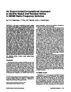
If ψ0 | R0 (g), the computation of v(g(θp )) can be based on the following proposition, which is easily deduced from [HN08, Prop.3.5] and [HN08, Cor.3.2]. Proposition 2.1. Let p, fp (x), θp be as above. Let t be a type of order R dividing fp (x), and let g(x) ∈ Z[x] be a nonzero polynomial. For any 1 ≤ i ≤ R, take a line Lλi of slope λi far below Ni (g), and let it shift upwards till it touches the polygon for the first time. Let S be the intersection of this line with Ni (g), let (s, u) be the coordinates of the left end point of S, and let H = u + s|λi | be the ordinate at the origin of this line. Then, (1) v(g(θp )) ≥ H/e1 · · · ei−1 , and equality holds if and only if Trunci (t) ∤ g(x). (2) If equality holds, then v(g(θp )) = v(Φi (θp )s πi (θp )u ) and   g(θp ) = Ri (g)(zi ) 6= 0. lredp Φi (θp )s πi (θp )u



Figure 1 shows that the segment S may eventually be reduced to a point. In this case, the residual polynomial Ri (g)(y) is a constant [HN08, Def.2.21], so that Trunci (t) ∤ g(x) automatically holds. A Ni (g) HH A H H A• HH S @ @ H•P u P H H Lλ HHi

A Ni (g) H HH A H HH A HAH u •H S H HH H•H P P HH Lλ i s

s

Figure 1 We may compute vp (g(θ)) = e(p/p)v(g(θp )) by applying Proposition 2.1 to the type tp . If for some 1 ≤ i ≤ r + 1, the truncated type Trunci (tp ) does not divide g(x), we compute v(g(θp )) as indicated in item 1 of this proposition. Nevertheless, it may occur that Trunci (tp ) divides g(x) for all 1 ≤ i ≤ r + 1 (for instance, if g(x) is a multiple of φp (x) = φr+1 (x)). In this case, we compute an improvement of the Montes approximation φp (x) by applying the single-factor lift routine [GNP10]; then, we replace the (r + 1)-th level of tp by the invariants (4) determined by the new choice of φr+1 (x) = φp (x), and we test again if tp = Truncr+1 (tp ) divides g(x).

A NEW COMPUTATIONAL APPROACH TO IDEAL THEORY IN NUMBER FIELDS

11

If tp divides g(x), then φp (x) is simultaneously close to a p-adic irreducible factor of f (x) and to a p-adic irreducible factor of g(x); hence, if f (x) and g(x) do not have a common p-adic irreducible factor, after a finite number of steps the renewed type tp will not divide g(x). On the other hand, if f (x) and g(x) have a common p-adic irreducible factor, they must have a common irreducible factor in Z[x] too; since f (x) is irreducible, necessarily f (x) divides g(x) and g(θ) = 0. We may summarize the routine to compute vp (α) as follows. Input: α ∈ K ∗ and a prime ideal p determined by a type tp of order r + 1. Output: vp (α). Write α = ab g(θ), with a, b coprime integers and g(x) ∈ Z[x] primitive. Compute ν = v(a/b). if ψ0 ∤ R0 (g) then return vp (α) = e(p/p)ν. for i = 1 to r + 1 do compute Ni− (g), Ri (g), and the ordinate H of Proposition 2.1. if ψi ∤ Ri (g) then return vp (α) = e(p/p)((H/e1 · · · ei−1 ) + ν). end for. 5. while ψr+1 | Rr+1 (g) do improve φp and compute the new values λr+1 , ψr+1 . − compute Nr+1 (g), Rr+1 (g), and the ordinate H of Proposition 2.1. end while. 6. return vp (α) = e(p/p)((H/e1 · · · er ) + ν).

1. 2. 3. 4.

2.2. Factorization of fractional ideals. For any α ∈ K ∗ , the factorization of the principal ideal generated by α is Y αZK = pvp (α) . p

Let α = (a/b)g(θ), for some positive coprime integers a, b and some primitive polynomial g(x) ∈ Z[x]. Then, vp (α) = 0 for all prime ideals p whose underlying prime number p does not divide the product ab NK/Q (g(θ)) = ab Resultant(f, g). Also, if p is a prime ideal of K and a, b are fractional ideals, we have vp (a + b) = min{vp (a), vp (b)}. Thus, the p-adic valuation of the fractional ideal a generated by α1 , . . . , αm ∈ K ∗ is: vp (a) = min1≤i≤m {vp (αi )}. After these considerations, it is straightforward to deduce a factorization routine of fractional ideals from the routines computing prime ideal decompositions of prime numbers and p-valuations of elements of K ∗ with respect to prime ideals p. Input: a family α1 , . . . , αm ∈ K ∗ of generators Q of a fractional ideal a. Output: the prime ideal decomposition a = p pap .

1. For each 1 ≤ i ≤ m, write αi = (ai /bi )gi (θ), with ai , bi coprime integers and gi (x) ∈ Z[x] primitive; then compute Ni = NK/Q (gi (θ)). 2. Compute N = gcd(a1 N1 , . . . , am Nm ) and M = lcm(b1 , . . . , bm ). 3. Factorize N and M and store all their prime factors in a list P. 4. For each p ∈ P apply Montes algorithm to obtain the prime ideal decomposition of p, and for each p|p, take ap = min1≤i≤m {vp (αi )}. 5. Return the list of pairs [p, ap ] for all p with ap 6= 0.

` GUARDIA, MONTES, AND NART

12

The bottleneck of this routine is step 3. We get a fast factorization routine in the number field K, as long as the integers N , M attached to the ideal a may be easily factorized. 3. Computation of generators In [GMN08, Sec.4] we gave an algorithm to compute generators of the prime ideals as certain rational functions of the φ-polynomials. Some inversions in K, one for each prime ideal, were needed. These inversions dominated the complexity of the algorithm, and they were a bottleneck that prevented the computation of generators for number fields of large degree. In sections 3.1 and 3.2 we construct a two-element representation of prime ideals, which does not need any inversion in K. As a consequence, this construction works extremely fast in practice even for number fields of large degree (see section 6). In section 3.3 we easily derive two-element representations of fractional ideals. For any prime ideal p of K we keep the notations for tp , fp (x), φp (x), Fp , θp , Kp , ZKp , as introduced in section 2. 3.1. Local generators of the prime ideals. Definition 3.1. A pseudo-generator of a prime ideal p of K is an integral element π ∈ ZK such that vp (π) = 1. Let p be a prime number, and let p = [p; φ1 , . . . , φr , φp ] be a prime ideal factor of pZK , corresponding to an f -complete type tp with an added (r + 1)-th level, as indicated in section 1.4. In this section we show how to compute a pseudogenerator of p from the secondary invariants ui , Quoti , of tp , for 1 ≤ i ≤ r, computed along the flow of Montes algorithm as indicated in (2). For each level 1 ≤ i ≤ r, let us denote: Quoti = [Qi,0 (x), . . . , Qi,ei −1 (x)]. Recall that Qi,0 (x) = 1, and for 0 < j < ei , the polynomial Qi,j (x) ∈ Z[x] is the (si − j)-th quotient of the φi -adic development of f (x) (cf. (1)), where si is the abscissa of the right end point of the side of slope λi of Ni− (f ). Also, let us define Hi,0 = 0,

Hi,j =

ui + j(|λi | + vi (φi )) , e1 · · · ei−1

∀ 0 < j < ei .

Proposition 3.2. For each level 1 ≤ i ≤ r and subindex 0 ≤ j < ei : (1) vq (Qi,j (θ)) ≥ e(q/p)Hi,j , for all prime ideals q | p. (2) vp (Qi,j (θ)) = e(p/p)Hi,j . Proof. Item 1 being proved in [GMN09a, Prop.10], let us prove item 2. Fix a level 1 P ≤ i ≤ r and a subindex 0 ≤ j < ei . Let ℓi = ordψi−1 Ri−1 (f ), and let f (x) = s≥0 as φsi be the φi -adic development of f (x). The Newton polygon of i-th order of f (x), Ni (f ), is the lower convex envelope of the cloud of points (s, vi (as φsi )), for all s ≥ 0. The principal part Ni− (f ) is equal to Ni (f ) ∩ ([0, ℓi ] × R); the typical shape of this polygon is illustrated in Figure 2. Let Sλi be the side of slope λi of this polygon, and si the abscissa of the right end point of Sλi .

A NEW COMPUTATIONAL APPROACH TO IDEAL THEORY IN NUMBER FIELDS

• JJ J H....... J

..... J.•.P .

vi (f )

13

N − (f )

i PP S PPλi PP PP P◦P •...... PP..•..h hhhh hhhh •

t

si − ei

0



si

Figure 2

-

ℓi

Ni− (qt φti )

For any 0 ≤ t ≤ ℓi , let qt (x) be the t-th quotient of the φi -adic development (see (1)). We have f (x) = qt (x)φi (x)t + rt (x), with X X rt (x) = as (x)φi (x)s , qt (x)φi (x)t = as (x)φi (x)s . 0≤s 1, we can always find a pseudo-generator of p by computing a suitable product of quotients in the lists Quoti , divided by a suitable power of p.

` GUARDIA, MONTES, AND NART

14

Corollary 3.3. (1) Let j1 , . . . , jr be subindices satisfying, 0 ≤ ji < ei , for all 1 ≤ i ≤ r. Then, the following element belongs to ZK : πj1 ,...,jr := Q1,j1 (θ) · · · Qr,jr (θ)/p⌊H1,j1 +···+Hr,jr ⌋ . (2) If e(p/p) > 1, there is a unique family j1 , . . . , jr as above, for which vp (πj1 ,...,jr ) = 1. This family may be recursively computed as follows: jr ≡ h−1 (mod er ), r resr := (jr hr − 1)/er , jr−1 ≡ −h−1 r−1 (ur + jr vr (φr ) + resr ) (mod er−1 ), resr−1 := (jr−1 hr−1 + ur + jr vr (φr ) + resr )/er−1 , ··· ··· −1 j1 ≡ −h1 (u2 + j2 v2 (φ2 ) + res2 ) (mod e1 ). Proof. Item 1 is an immediate consequence of item 1 of Proposition 3.2. Also, by Proposition 3.2, vp (πj1 ,...,jr ) = e(p/p) (H1,j1 + · · · + Hr,jr − ⌊H1,j1 + · · · + Hr,jr ⌋) . Thus, item 2 states that there is a unique family j1 , . . . , jr such that 1 (mod Z). H1,j1 + · · · + Hr,jr ≡ e(p/p) Since e(p/p) = e1 · · · er and |λi | = hi /ei , this is equivalent to: u1 + j1 v1 (φ1 )+

j1 h1 + u2 + j2 v2 (φ2 ) + ··· e1 jr−1 hr−1 + ur + jr vr (φr ) jr hr 1 ···+ + ≡ (mod Z). e1 · · · er−1 e1 · · · er e1 · · · er

Clearly this congruence has a unique solution j1 , . . . , jr satisfying 0 ≤ ji < ei , for all 1 ≤ i ≤ r, and this solution may be recursively obtained by the procedure described in item 2.  The only property of tp that we used in in Corollary 3.3 is: e1 · · · er = e(p/p). Thus, we don’t need to use all levels of tp to compute a pseudo-generator of p; in practice we take r to be the minimum level such that e1 · · · er = e(p/p). 3.2. Generators of the prime ideals. Let p be a prime number, and P the set of prime ideals of K lying over p. Once we have pseudo-generators πp ∈ p of all p ∈ P, in order to find generators we need only to compute a family of integral elements, {bp ∈ ZK }p∈P , satisfying: (10)

vp (bp ) = 0, ∀ p ∈ P,

vq (bp ) > 1, ∀ q, p ∈ P, q 6= p.

Then, for each p ∈ P, the integral element: X αp := bp πp +

bq ∈ ZK

q∈P,q6=p

clearly satisfies: vp (αp ) = 1, vq (αp ) = 0, for all q 6= p. Therefore, p is the ideal generated by p and αp . The rest of this section is devoted to the construction of these multipliers {bp }.

A NEW COMPUTATIONAL APPROACH TO IDEAL THEORY IN NUMBER FIELDS

15

Let (tp )p∈P be the parameterization of the set P by a family of f -complete types obtained by an application of Montes algorithm. As usual, we suppose that each tp has been conveniently enlarged with an (rp + 1)-th level, as indicated in section 1.4. From now on we provide the invariants of tp with a subscript p to distinguish the prime ideal they belong to: rp , φi,p , mi,p , λi,p , etc. The integral elements bp will be constructed as suitable products of φ-polynomials divided by suitable powers of p. The crucial ingredient is Proposition 3.8, that computes vp (φi,q (θ)) for all p 6= q in P, and all 1 ≤ i ≤ rq + 1. Definition 3.4. For any pair p, q ∈ P, we define the index of coincidence between the types tp and tq as:  0, if ψ0,p 6= ψ0,q , i(tp , tq ) = min {j ∈ Z>0 | (φj,p , λj,p , ψj,p ) 6= (φj,q , λj,q , ψj,q )} , if ψ0,p = ψ0,q . Alternatively, i(tp , tq ) is the least subindex j for which Truncj (tp ) 6= Truncj (tq ). Remark 3.5. By definition, φi,p = φi,q ,

λi,p = λi,q ,

ψi,p = ψi,q ,

∀ i < i(tp , tq ).

Hence, by the definition of the p-adic valuations vi,p , vi,q , and by [HN08, Thm. 2.11], we get: vi,p = vi,q ,

mi,p = mi,q ,

vi,p (φi,p ) = vi,q (φi,q ),

∀ i ≤ i(tp , tq ).

Lemma 3.6. If p, q ∈ P, and p 6= q, then i(tp , tq ) ≤ min{rp , rq }. Proof. Suppose rp ≤ rq and i(tp , tq ) = rp + 1. Then, Truncrp (tp ) = Truncrp (tq ). Since the type Truncrp (tp ) is f -complete, it singles out a unique p-adic irreducible factor of f (x) (item 2 of Definition 1.1). Hence, Truncrp (tq ) is also f -complete and it singles out the same p-adic irreducible factor of f (x). This implies that p = q.  By (7) and (9), for all 1 ≤ i ≤ rp + 1 we have (11)

vp (φi,p (θ)) = e(p/p)

vi,p (φi,p ) + |λi,p | . e1,p · · · ei−1,p

In order to compute the values of vp (φi,q (θ)), for p 6= q, we need still another definition. Definition 3.7. Let p, q ∈ P, q 6= p, and j = i(tp , tq ). Let sp = # Refinementsj,p , and consider the list Ref p obtained by extending the list Refinementsj,p by adding the pair [φj,p , λj,p ] at the last position: i i i h i h hh (s +1) (s +1) (s ) (s ) (1) (1) := [φj,p , λj,p ] . Ref p = φj,p , λj,p , · · · , φj,pp , λj,pp , φj,pp , λj,pp Let Ref q be the analogous list for the prime ideal q. We define the greatest common φ-polynomial of the pair (tp , tq ) to be the more advanced common φ-polynomial in the two lists Ref p , Ref q . We denote it by: (k)

(k)

φ(p, q) := φj,p = φj,q , (k)

(k)

for the maximum index k such that φj,p = φj,q . (k)

(k)

We define the hidden slopes of the pair (tp , tq ) to be: λqp := λj,p , λpq := λj,q .

` GUARDIA, MONTES, AND NART

16

Remarks. (1) By the concrete way the processes of branching, enlarging and/or refining were defined, this polynomial φ(p, q) always exists. In fact, let us show that we must (1) (1) have φj,p = φj,q . Since Truncj−1 (tp ) = Truncj−1 (tq ), this type had some original representative (say) φj . By considering Nφ−j ,vj (f ) and the irreducible factors of all residual polynomials of all sides, we had different branches (λ, ψ) to analyze; if there was only one branch, the algorithm necessarily performed a refinement step, because otherwise we would have i(tp , tq ) > j. After eventually a finite number of these unibranch refinement steps (that were not stored in the list Refinementsj ), we considered some representative, let us call it φj again, leading to several branches. One of these branches led later to the type tp and one of them (maybe still the same) to the type tq . If the p-branch experimented refinement, the list Refinementsj,p had (1) φj,p = φj as its initial φ-polynomial; if the p-branch was f -complete or had to be enlarged, then the list Refinementsj,p remained empty and we had φj,p = φj . In any case, φj is the first φ-polynomial of the list Ref p . (ℓ)

(ℓ)

(2) All φj,p , φj,q are representatives of tj−1 := Truncj−1 (tp ) = Truncj−1 (tq ); in particular, all these polynomials have degree mj . With the obvious meaning for (ℓ) ψj,p , we have necessarily: i i h i h i h h (ℓ) (ℓ) (ℓ) (ℓ) (ℓ) (ℓ) (k) (k) (k) (k) (k) (k) φj,p , λj,p , ψj,p = φj,q , λj,q , ψj,q , φj,p , λj,p , ψj,p 6= φj,q , λj,q , ψj,q , for all 1 ≤ ℓ < k. Thus, φ(p, q) is the first representative of tj−1 for which the branches of tp and tq are different.

(3) Caution: we may have Ref p = Ref q . In this case φ(p, q) = φj,p = φj,q and λqp = λj,p = λj,q = λpq ; the branches of tp and tq are distinguished by ψj,p 6= ψj,q . Proposition 3.8. Let p, q ∈ P, p 6= q, and j = i(tp , tq ). Let φ(p, q) be the greatest common φ-polynomial of the pair (tp , tq ) and λqp , λpq the hidden slopes. For any 1 ≤ i ≤ rq + 1,      0, if j = 0,       vi (φi ) + |λi |   , if i < j,    e1 · · · ei−1   vp (φi,q (θ))  vj (φj ) + |λqp | = , if i = j and φj,q = φ(p, q),  e1 · · · ej−1 e(p/p)      vj (φj ) + min{|λqp |, |λpq |}   , if i = j and φj,q 6= φ(p, q),   e1 · · · ej−1    q p   mi,q vj (φj ) + min{|λp |, |λq |}   · , if i > j > 0.  mj e1 · · · ej−1 In these formulas we omit the subscripts p, q when the invariants of the two types coincide (cf. Remark 3.5). Proof. The case j = 0 was seen in (8). The cases i < j and i = j, φj,q = φ(p, q), are a consequence of (11).

A NEW COMPUTATIONAL APPROACH TO IDEAL THEORY IN NUMBER FIELDS

17

Suppose i > j > 0 and φj,p = φj,q ; we have then, φ(p, q) = φj,p = φj,q and λqp = λj,p , λpq = λj,q . We compute vp (φi,q (θ)) by applying Proposition 2.1 to the polynomial g(x) = φi,q (x) and the type tp . Since vj,p = vj,q and φj,p = φj,q , we have Nj,p (φi,q ) = Nj,q (φi,q ). On the other hand, we saw in the proof of Lemma 1.2 that Nj,q (φi,q ) is one-sided of slope λj,q . Figure 3 shows the three possibilities for the line Lλj,p of slope λj,p that first touches Nj,p (φi,q ) from below. ... ... ... ... H• ... ... @ @ ... ... ...@λj,q ...

... ..

.. H•

@ Lλj,p

vj (φi,q ) 0

@•

mi,q /mj

λj,p < λj,q

vj (φi,q ) 0

@ @ @λj,q @ @•... ..

.. Lλj,p

mi,q /mj

λj,p = λj,q

• @ @ ...... λj,q H .........@ ..... ..@ ...... ..... @.•........Lλj,p vj (φi,q ) ... ..

0

mi,q /mj

λj,p > λj,q

Figure 3 A glance at Figure 3 shows that mi,q mi,q H = vj (φi,q ) + min{|λj,p |, |λj,q |} = (vj (φj ) + min{|λj,p |, |λj,q |}), mj mj the last equality by Lemma 1.2. Now, if λj,p 6= λj,q , the line Lλj,p touches the polygon only at one point, and the residual polynomial Rj,p (φi,q )(y) is a constant. If λj,p = λj,q , then Lλj,p contains Nj,p (φi,q ) and Rj,p (φi,q ) = Rj,q (φi,q ) is a power of ψj,q , up to a multiplicative constant. In this case, necessarily ψj,q 6= ψj,p , by the definition of j = i(tp , tq ). Therefore, Truncj (tp ) never divides φi,q , and Proposition 2.1 shows that v(φi,q (θp )) = H/(e1 · · · ej−1 ). By (7), we get the desired expression for vp (φi,q (θ)). Suppose now i > j > 0, φj,p 6= φj,q , or i = j, φj,q 6= φ(p, q). Consider a new type ˜tp , constructed as follows: if φj,p = φ(p, q), we take ˜tp = tp , and if φj,p 6= φ(p, q), we take ˜tp = (φ1 ; λ1 , φ2 ; · · · , φj−1 ; λj−1 , φ(p, q); λqp , φj,p ; λj,p − λqp , φj+1,p ; λj+1,p , · · · , φrp +1,p ; λrp +1,p , ψrp +1,p ). By [GMN08, Cor.3.6], ˜tp is a type, and it is also f -complete. If φj,p 6= φ(p, q) then ˜tp is not optimal because deg φ(p, q) = deg φj,p , but optimality is not necessary to apply Proposition 2.1. We consider an analogous construction for ˜tq . The new types satisfy i(˜tp , ˜tq ) = j and they have the same j-th φ-polynomial; finally if i = j, the polynomial φi,q is the (j + 1)-th φ-polynomial of ˜tq . Therefore, the computation of vp (φi,q ) is deduced by the same arguments as above.  We are ready to construct the family {bp }p∈P . Consider the following equivalence relation in the set P: p ∼ q ⇐⇒ ψ0,p = ψ0,q , and denote by [p] the class of any p ∈ P. For each class [p], let φ1,[p] (x) ∈ Z[x] be the first φ-polynomial in any list Ref q for some q ∈ [p]; we saw in the first remark following Definition 3.7 that all lists

` GUARDIA, MONTES, AND NART

18

Ref q , for q ∈ [p], have the same initial φ-polynomial. Now, for each q ∈ [p], denote by λ01,q the first slope in the list Ref q . In other words, for any q ∈ [p], we have   (φ1,q , λ1,q ), if Refinements1,q is empty,   (φ1,[p] , λ01,q ) = (1) (1)  φ ,λ if Refinements1,q is not empty. 1,q 1,q , By (8) and (9), (12)

vq (φ1,[p] (θ)) =

(

0, e(q/p)|λ01,q |,

if q 6∈ [p], if q ∈ [p].

Consider now, for each class [p]: B[p] (x) :=

Y

φ1,[q] (x).

[q]6=[p]

Fix a prime ideal p ∈ P. If #[p] = 1, the element bp = (B[p] (θ))2 satisfies (10) already. Suppose now #[p] > 1. For all l ∈ [p], l 6= p, let φl = φrl +1,l be the Montes approximation to fl (x) contained in tl ; consider the least positive numerator and denominator of the rational number vp (φl (θ))/e(p/p) (which has been computed in Proposition 3.8): vp (φl (θ)) nl = , gcd(nl , dl ) = 1. e(p/p) dl We look for an integral element of the form: Q (B[p] (θ))m l∈[p], l6=p φl (θ)dl , (13) bp = pN where the exponents N, m are given by N=

X

nl ,

m=

l∈[p], l6=p

&

max

q∈P, q6∈[p]

(

N e(q/p) + 2 e(q/p)|λ01,q |

)'

.

Take q 6∈ [p]. By (8) and (12), we have   Y φl (θ)dl  = 0, vq (B[p] (θ)) = vq (φ1,[q] (θ)) = e(q/p)|λ01,q|. vq  l∈[p], l6=p

Hence, vq (pN bp ) = m e(q/p)|λ01,q| ≥ N e(q/p) + 2, so that vq (bp ) > 1, as desired. For the prime p itself, we have vp (B[p] (θ)) = 0 and, by construction,   X dl vp (φl (θ)) − N e(p/p) = 0. vp (bp ) =  l∈[p], l6=p

Finally, for a prime l ∈ [p], l 6= p, we have vl (B[p] (θ)) = 0 and X vl (φl′ (θ)dl′ ), V2 := vl (φl (θ)dl ). vl (bp ) = V1 + V2 − N e(l/p), V1 := l′ ∈[p], l′ 6=p,l

Lemma 3.6 and Proposition 3.8 show that V1 (as all invariants we used so far) depends only on the numerical invariants of the types tl , tl′ , of level 1 ≤ i ≤ i(tl , tl′ ) ≤ min{rl , rl′ }, and not on the quality of the Montes approximations φl′ .

A NEW COMPUTATIONAL APPROACH TO IDEAL THEORY IN NUMBER FIELDS

19

On the other hand, V2 depends on the choice of φl as a Montes approximation of fl(x); by (11): V2 = vl (φl (θ)dl ) = dl e(l/p)

vrl +1,l(φl ) + hrl +1,l = dl (vrl +1,l (φl ) + hrl +1,l ). e1,l · · · erl ,l

Hence, for all l ∈ [p], l 6= p, we improve the Montes approximation φl till we get hrl +1,l ≥

2 + N e(l/p) − V1 − vrl +1,l (φl ). dl

This ensures that vl (bp ) > 1, as desired. 3.3. Two-element representation of a fractional ideal. Any fractional ideal a of K admits a two-element representation: a = (ℓ, α), where α ∈ K and ℓ = ℓ(a) ∈ Q is the least positive rational number contained in a. It is straightforward to obtain such a representation from the two-element representation of the prime ideals obtained in the last section. For the sake of completeness we briefly describe the routine. For each prime ideal p of K, we have computed an integral element αp ∈ ZK such that vp (αp ) = 1,

vq (αp ) = 0, ∀ q|p, q 6= p.

These elements are of the form: αp = pνp hp (θ), where νp ∈ Z and hp (x) ∈ Z[x] is a primitive polynomial. Generically, νp ≤ 0, except for the special case p = pZK , where νp = 1, hp (x) = 1. Let us write NK/Q (hp (θ)) = pµp Np , with p ∤ Np . Q Suppose first that a = p|p pap has support only in prime ideals dividing p. We take then:    Y a Y |a | ap p p Np , H := max αp α= . e(p/p) p|p a 0, we look for the first index, 1 ≤ i ≤ r + 1, for which the truncation Trunci (t) does not divide g(x). In the paragraph following Proposition 2.1 we showed that this will always occur, eventually (for i = r + 1) after improving the Montes approximation φp = φr+1 . By Proposition 2.1, there is a computable point (s, u) ∈ Ni (g) such that v(g(θp )) = (shi + uei )/(e1 · · · ei ) = v(Φi (θp )s πi (θp )u ), and   g(θp ) = Ri (g)(zi ) 6= 0. lredp Φi (θp )s πi (θp )u Now, if (shi +uei )/(e1 · · · ei ) > N , we have lredp (g(θp )/pN ) = 0; on the other hand, if (shi + uei )/(e1 · · · ei ) = N , we have     g(θp ) Φi (θp )s πi (θp )u (14) lredp = Ri (g)(zi ) · lredp = Ri (g)(zi ) z1t1 · · · ziti , pN pN

A NEW COMPUTATIONAL APPROACH TO IDEAL THEORY IN NUMBER FIELDS

21

where p−N Φi (θp )s πi (θp )u = γ1t1 · · · γiti , and the vector (t1 , . . . , ti ) ∈ Zi can be found by the procedure of Lemma 1.4, applied to the input vector
log p−N Φi (x)s πi (x)u = (−N, 0, . . . , 0) + s log Φi + u log πi .

Since log Φi , log πi have been stored as secondary invariants of tp , we get in this way a really fast computation of lredp (p−N g(θp )). This ends the computation of the reduction modulo p map redp .

4.2. Chinese remainder theorem. It is straightforward to design a chinese remainders routine once the following problem is solved. Problem. Let p be a prime number, P the set of prime ideals of K lying above p, and (ap )p∈P a family of non-negative integers. Find a family (cp )p∈P of integral elements cp ∈ ZK such that, cp ≡ 1 (mod pap ),

cp ≡ 0 (mod qaq ), ∀ q ∈ P, q 6= p,

for all p ∈ P. There is an easy solution to this problem: take the element bp ∈ ZK satist fying (10), constructed in section 3.2, and consider cp = (bp )p (qp −1) , where qp = NK/Q (p) = #Fp , and t is sufficiently large. However, the element cp constructed in this way is not useful for practical purposes because it may have a huge norm and a huge height (very large numerators or denominators of the coefficients of its standard representation as a polynomial in θ), if qp or t are large. Instead, we shall refine the construction of the element bp to get a small size solution cp to the above problem. First we deal with the particular case ap = 1. The idea is to get an element bp ∈ ZK satisfying vp (bp ) = 0,

vq (bp ) ≥ aq , ∀ q ∈ P, q 6= p,

and then find β ∈ K such that vp (β) = 0, cp := bp β is integral, and cp ≡ 1 (mod p). Since we know the Q two-element representation q = (p, αq ) of the prime ideals, we could take bp = q∈P, q6=p (αq )aq . Again, this might lead to a bp with large size, so that a direct construction of bp is preferable in order to keep its size as small as possible. Thus, we consider an element bp ∈ ZK as in (13): Q (B[p] (x))m l∈[p], l6=p φl (x)dl bp = , pN P P with N = l∈[p], l6=p dl v(φl (θp )) = l∈[p], l6=p nl . By construction, vp (bp ) = 0. Let i = maxq∈P, q6=p {i(tp , tq )}; Lemma 3.6 shows that i ≤ rp . From now on, we use only invariants of the type tp and we drop the subindex p in the notation. Let  if i = 0,  0,   vi+1 (φi+1 )) M= , if i > 0.  e1 · · · ei

Arguing as in section 3.2, we can take m sufficiently large, and each φl (x) sufficiently close to the p-adic irreducible factor fl (x), so that (15)

vq (bp ) ≥ aq + M e(q/p), ∀ q ∈ P, q 6= p,

` GUARDIA, MONTES, AND NART

22

while keeping the denominator pN and the condition vp (bp ) = 0. In particular, bp belongs to ZK . The idea is to multiply bp by some element in K that conveniently modifies its residue class modulo p. We split this task into two parts, that may be considered as a kind of respective inversion modulo p of (B[p] (θ))m and Q p−N l∈[p], l6=p φl (θ)dl . Let h(x) = (B[p] (x))m . Then, ζ := redp (h(θ)) ∈ F1 ⊆ Fp is just the class of h(x) modulo the ideal (p, φ1 (x)). We invert ζ in F1 and represent the inverse ζ −1 = P (z0 ), as a polynomial in z0 of degree less than f0 , with coefficients in the prime field F0 . Take β0 = P (θ), where P (x) ∈ Z[x] is an arbitrary lift of P (x); clearly, h(θ)β0 ≡ 1 (modQ p). Let now g(x) = p−N l∈[p], l6=p φl (x)dl . If [p] = {p}, then i = 0, N = M = 0, g(x) = 1 and we are done. Suppose [p] ! {p}, so that 1 ≤ i ≤ rp . By the definition of the index of coincidence, we have Trunci (tp ) ∤ φl (x), for all l 6= p; by the Theorem of the product [HN08, Thm.2.26], Trunci (tp ) ∤ g(x). Therefore, as we saw in the last section, ξ := lredp (p−N g(θp )) = Ri (g)(zi ) z1t1 · · · ziti ∈ Fi+1 , for some easily computable sequence of integers (t1 , . . . , ti ). Let V = e1 · · · ei M ; by
[HN08, Cor.3.2], v πi+1 (θp )V = M . Compute a vector (t′1 , . . . , t′i ) ∈ Zi such that t′

t′

p−M πi+1 (x)V = γ11 · · · γi i , as indicated in Lemma 1.4, and take t′

t′

ξ ′ := z11 · · · zi i ∈ Fi+1 . Let ϕ(y) ∈ Fi [y] be the unique polynomial of degree less than fi , such that ϕ(zi ) = ℓ V /e zi i i (ξξ ′ )−1 . Let ν = ordy ϕ(y). Clearly, V ≥ vi+1 (φi+1 ) = ei fi vi+1 (φi ), the last equality by [HN08, Thm.2.11]. Therefore, we can apply the constructive method described in [HN08, Prop.2.10] to compute a polynomial P (x) ∈ Z[x] satisfying the following properties: deg P (x) < mi+1 ,

vi+1 (P ) = V,

y ν Ri (P )(y) = ϕ(y).

A look at the proof of [HN08, Prop.2.10] shows that Ni (P ) is one sided of slope λi and its end points have abscissa ei ν and ei deg ϕ (cf. Figure 4). V /ei

H HH •H H Ni (P ) H HH HH H H H•H HH Lλ Hi ei ν

ei deg ϕ

Figure 4 Claim: lredp (p−M P (θp )) = ξ −1 . In fact, since deg P (x) < mi+1 and vi+1 (P ) = V , the Newton polygon Ni+1 (P ) is the single point (0, V ); in particular, Trunci+1 (tp ) does not divide P (x) and Proposition 2.1 shows that v(P (θp )) = M and
lredp P (θp )/πi+1 (θp )V = Ri+1 (P )(zi+1 ) 6= 0.

A NEW COMPUTATIONAL APPROACH TO IDEAL THEORY IN NUMBER FIELDS

23

Actually, Ri+1 (P )(y) has degree 0 and it represents a constant in Fi+1 that we denote simply by Ri+1 (P ). By (14),
lredp p−M P (θp ) = Ri+1 (P ) lredp (p−M πi+1 (θp )V ) = Ri+1 (P ) ξ ′ . By the very definition of the residual polynomial [HN08, Defs.2.20+2.21], we have (ei ν−ℓi V )/ei

Ri+1 (P ) = zi

−ℓi V /ei

Ri (P )(zi ) = zi

ϕ(zi ) = (ξξ ′ )−1 ,

and the Claim is proven. Finally, consider cp = bp β0 (p−M P (θ)). The condition (15) ensures that cp belongs to ZK (although p−M P (θ) might not be integral) and satisfies vq (cp ) ≥ aq , for all q ∈ P, q 6= p. By construction, redp (cp ) = lredp (ιp (cp )) = 1. It remains to solve our Problem when ap > 1. In this case, we find c ∈ ZK such that c ≡ 1 (mod p), c ≡ 0 (mod qaq ), ∀ q ∈ P, q 6= p, and we take cp = (c − 1)m + 1, where m is the least odd integer that is greater than or equal to ap /vp (c − 1). 5. p-integral bases Let p be a prime number and let Fp be the prime field of characteristic p. A p-integral basis of K is a family of n Z-linearly independent integral elements α1 , . . . , αn ∈ ZK such that 


p ∤ ZK : α1 , . . . , αn Z ,

or equivalently, such that the family α1 ⊗ 1, . . . , αn ⊗ 1 is Fp -linearly independent in the Fp -algebra ZK ⊗Z Fp . If the discriminant disc(f ) of f (x) may be factorized, the computation of an integral basis of K (a Z-basis of ZK ) is based on the computation of p-integral bases for the different primes p that divide disc(f ). Anyhow, even when disc(f ) may not be factorized, the computation of a pintegral basis of K for a given prime p is an interesting task on its own. In this section we show how to carry out this task from the data captured by the OkutsuMontes representations of the prime ideals p lying over p. For any such prime ideal we keep the notations for fp (x), φp (x), Fp , θp , Kp , ZKp , as introduced in section 2. 5.1. Local exponent of a prime ideal. Let P be the set of prime ideals lying over p. For any p ∈ P we fix the topological embedding K ֒→ Kp determined by sending θ to θp . Definition 5.1. We define the local exponent of p ∈ P to be the least positive integer exp(p) such that pexp(p) ZKp ⊆ Zp [θp ]. Note that exp(p) is an invariant of the irreducible polynomial fp (x) ∈ Zp [x], but it is not an intrinsic invariant of p.

` GUARDIA, MONTES, AND NART

24

The computation of exp(p) is easily derived from the results of [GMN09b]. Let p = [p; φ1 , . . . , φr , φp ] be the Okutsu-Montes representation of p, as indicated in section 1.4. By [GMN09b, Lem.4.5]: fp (x) ≡ φp (x) (mod m⌈ν⌉ ),

where ν = νp + (hr+1 /e(p/p)),

and νp is the rational number h1 h2 hr + + ···+ . e1 e1 e2 e1 · · · er

νp :=

Caution: this number is not always an invariant of fp (x). If er fr = 1, the Okutsu depth of fp (x) is R = r − 1 (cf. (3)), and hr depends on the choice of φr . Denote φ0 (x) = x, m0 = 1, mr+1 = np := e(p/p)f (p/p). Any integer 0 ≤ m < np can be written in a unique way as: m=

r X

a i mi ,

0 ≤ ai