A New Neural Network Based FOPID Controller Naser Sadati, Alireza Ghaffarkhah, Sarah Ostadabbas Abstract- Fractional order PID controllers are suitable for almost all types of dynamic models. In this paper, a new adaptive fractional order PID controller using neural networks is introduced.The overall performance using the proposed adaptive fractional order PID controller is demonstrated through some examples. It is shown that the new controller scheme can give excellent performance and more robustness in comparison with the conventional controllers like GPC. I. INTRODUCTION
The basic idea of extending the classical integer order calculus to non-integer order cases in control systems is not new. The earliest systematic studies seem to have started in the beginning and middle of the 19th century by Letnikov, Riemann and Liouville, as stated in [1]. Reader can find some examples of common applications of fractional order differentiation in [1]. This new concept has also attracted researchers in applied sciences. Many applications of fractional order differentiation can also be found in engineering[2]-[4]. In control engineering the fractional order differentiation can be used in either controller design or system identification. In the field of system identification, studies on real systems have revealed inherent fractional order dynamic behavior. The resulting fractional order dynamic models can replace the real plants more adequately than the integer order ones. They provide more adequate descriptions of many actual dynamical processes. In the field of automatic control, the fractional order controllers which are the generalization of classical integer order controllers, would lead to more precise and robust control performances. Although it is reasonably true, as also argued in [5], that the fractional order models require the fractional order controllers to achieve the best performance, but in most cases the researchers consider the fractional order controllers applied to regular linear or nonlinear dynamics to enhance the system control performances. Historically there are four major types of fractional order controllers [5]-[6]: - CRONE Controller - Tilted Proportional and Integral(TID) Controller - Fractional Order PID (PITD'D) Controller Naser Sadati is with Faculty of Electrical Engineering and Head of Intelligent Systems Laboratory, Department of Electrical Engineering, Sharif University of Technology, Tehran, Iran sadati@sharif. edu Alireza Ghaffarkhah is with the Intelligent Systems Laboratory, Department of Electrical Engineering, Sharif University of Technology, Tehran, Iran ghaffarkhah@ee. sharif .edu Sarah Ostadabbas is with the Department of Electrical Engineering, Sharif University of Technology, Tehran, Iran
[email protected]
- Fractional Order Lead-Lag Compensator
For a historical note and a comparative introduction of these four fractional order controllers, the readers can refer to [6],[7]. However, PIA D1 controller is the most distinguished controller among them. Meanwhile, many researchers have been trying to find a proper method to design and tune an FOPID controller [8]-[10]. Application of intelligent methods in designing FOPID controllers is quite new. In this paper a new approach for designing FOPID controllers will be introduced. A well-tuned neural network will adaptively change the coefficients of FOPID controller, namely A , ,u and its weights are found in order to minimize a well-defined cost function which is defined to be the overall mean-square error in this case. Finding A , ,u and neural network weights will lead us to a medium-scale unconstrained optimization problem which will be solved numerically. II. A BRIEF INTRODUCTION TO FRACTIONAL ORDER CALCULUS
There are mainly two different types of fractional order derivates. Letnikov, Riemann and Liouville definition (LRL definition) and Caputo definition[II]. These two definitions can be discussed from the view point of its use for the formulation and solution of applied problems leading to the differential equations of the fractional order. Here we will briefly introduce these two definitions knowing that the LRL definition is more distinguished than the Caputo definition. The LRL definition of fractional order derivatives can be expressed as [11]
LDat
a
( d .n
I
t
F(n a) Ut) (n-1 I
O)
(18)
The control signal u(t) can then be expressed in the time domain as
u(t) = Kpe(t) + KID- e(t) + KDD"e(t)
(19) important advantages of the PIADA
One of the most controller is its possibility for better control of fractional order dynamical systems. Another advantage lies in the fact that the PIADA controllers are less sensitive to changes of parameters of a controlled system [15]. This is due to the fact that having two extra degrees of freedom can better adjust the dynamical properties of fractional order control systems. In our controller A , ,u and Neural Network weights are determined optimally in learning phase to minimize a welldefined cost function. After the learning process, A and ,u remain fixed and FOPID coefficients (Kp, KI and KD) are changed adaptively as the error changes.
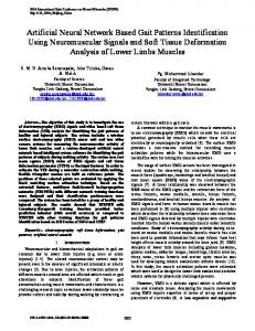
Fig. 1.
The basic architecture of an auto-tuning neuron.
The output ( of neuron is given by Ie -b.net (20) I +e-b.e where the activation function h: R --> R is a modified hyperbolic tangent function, a is the saturated level, and b is the slope of function. In our controller each neuron is dedicated to one of three FOPID coefficients, i.e. one neuron for KP, one for KI and one for KD. So totally there are eleven parameters to be determined including A and ,u . The overall structure of the controller is shown in Fig. 2.
0
=
h(net)
=
a.
brnet
uNs
Adap. FOPti) Cntl
Digitiz.d plant
d
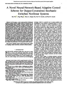
Fig. 2. The overall structure of the control system
As it can be seen in Fig. 2 (after specifying those eleven parameters) the FOPID coefficients are adaptively changed by the Neural Network as the error changes. As we mentioned before, in learning phase, the parameters are determined in order to minimize a previously defined cost function. It's obvious that the cost function we have selected, would affect the overall performance of the controller. Here, the total MSE (mean square error) of the closed-loop system to a unit step input is chosen as the cost function. Now by assuming that in the above closed-loop system, as shown in Fig. 2, we have a unit step input and the error e(k) is calculated for Q samples, the total MSE of the closed-loop system can be written as
MSE
=
Z Ee2(k)
(21)
k=l
where the Ith sample, is the first sample in which y(k) is not zero. Now by choosing a large Q, the overall performance of the controller can be improved; although it also increases
764
the time taken in learning phase. So by choosing Q, it must be a trade-off between performance of the controller and the time we require for the controller design. Now let's look at the closed-loop system as a black box. For a specific Q and unit step as the input reference, the MSE can be calculated for any combination of eleven parameters. As a result, finding A, ,u and also a, b and X of each neuron, will lead to a medium-scale unconstrained optimization problem which can be solved numerically. V. TUNING PARAMETERS USING A NUMERICAL OPTIMIZATION METHOD Generally, two conventional strategies namely analytical and numerical methods can be considered for optimization problems. In analytical method, the analytical formulation of the functions will be used to find gradient and/or Hessian matrix. If the exact formulation of the goal function is given (or can be easily calculated) then this kind of optimization will be much faster than the numerical methods. But in our case, it's too difficult to find the analytical formulation of the goal function, i.e. it is analytically hard to write MSE as a function of A, ,u and also a, b and X of each neuron. Consequently we decided to use the numerical methods of optimization. For this purpose, a simple version of NelderMead simplex search method and the BFGS (Broyden, Fletcher, Goldfarb, and Shanno) quasi-Newton method introduced in MATLAB optimization toolbox [17] was used. Different choices of line search strategies can be used for unconstrained minimization problems. The line search strategies use the safeguarded cubic and quadratic interpolation and extrapolation methods. Almost the most favored approach that uses the gradient information, is the quasi-Newton method. Actually this method builds up curvature information at each epoch to formulate a quadratic model of the problem. Newton-type methods calculate H (Hessian Matrix) directly and proceed in a selected direction of descent to find the minimum after a number of iterations. Calculating H directly involves a large amount of computation. Quasi-Newton methods avoid this by using the observed behavior of the goal function and its gradient, to build up the curvature information to make an approximation of H using an appropriate updating technique. A large number of Hessian updating methods have been developed ever since. MATLAB optimization toolbox uses the formula of Broyden [18], Fletcher [19] Goldfarb [20], and Shanno [21] (BFGS) to update the Hessian matrix when the gradient information is not provided. Using this updating formula, the authors have developed a toolbox which can find the minimums of the special goal functions much faster than MATLAB optimization toolbox. As we mentioned before, In BFGS quasi-Newton method we can focus on computing the Hessian matrix more cheaply than the other numerical methods. Lets assume Sk
=
Xm1+ -Xm
=
amvm
(22)
be the change in the parameters in the current iteration. Also
Tim
gm+ I -gm
(23)
be the change of the gradients, where
6'm
=
ifd (Xm)]I
(Xm)
(24)
and am is the so called step length. Then a natural estimate of the Hessian matrix at the next iteration, Hm±1+, would be the solution of the system of linear equations
Hm+Ism
(25)
Ti Tm
That is, Hmi+ is the ratio of the change in the gradient to the change in the parameters. This is called the quasi-Newton condition. There are many solutions to this set of equations. Broyden suggested a solution in the following form
Hm±+
=
(26)
Hm + uVT
Further works have also suggested to use the other types of updates, the most important of which are the DFP (Davidon, 1959, and Fletcher and Powell, 1963), and the BFGS. The BFGS is generally regarded as the best performing technique, written as T
THm
Hm Sm S
H±i =Hm + Tm m ST Hm Sm TmS'M
7171T TITM
H
Hm
+
(27)
gmmT
mgm mT CmHm5m. However, the update
Tim Sn m
T
with the fact that Hmsm = is made to the Cholesky factorization of H rather than to the Hessian itself, that is to R where H = RTR. The direction
6m is also computed to find a solution to the following relation (28) RTRmTm = gm
where Rm is the Cholesky factorization of Hm. In each epoch of optimization a line search algorithm must be used. The line search is used to find the value of am, such that
f (xm -amm) < (xm) Some common line search methods are; Fibonacci, Golden Section and Polynomial methods involving interpolation or extrapolation (e.g., quadratic, cubic). The line search is an essential part of the quasi-Newton optimization. In our preferred line search algorithm (simplex method or mixed Cubic/Quadratic polynomial method), at first step, am = 1 is tried. Then if the reduction of the function is sufficient, that is
If(XTn -6) -f(XTn)116'
gTn < -0001
(29)
The step length is set to one and the iterations continue. If not, a quadratic function is fit to f (xm -amm) using f(xm),gm and f(xm -m) , i.e. using the values of f(.) 0 and am = 1 and the gradient evaluated where am where am 0. If the value of am at the minimum of that quadratic passes the criterion, that value is selected for the step length. But if not, a cubic is fit to the above information plus an additional evaluation of the function with am set to a specified value. If that fails, new evaluations of the function with trial values of the step length are set to the value found
765
in the cubic fitting. This process continues either until a step length is found that satisfies the criteria, or until a specified number of attempts (for example 40 attempts) have been made. If this number of attempts have been made without finding a satisfactory step length, we try a random search. In the random line search, random trial values of the step length from within a set radius are tried. If any leads to the reduction of the function, then it is selected as the step length. For more precise explanation of this method and other line search methods, one can see[22]. VI. SIMULATION RESULTS In the following, two different popular chemical control processes are used to evaluate the control performance of the proposed controller scheme. In each example, the performance of the proposed controller is compared to the performance of GPC, a kind of model predictive controller, which widely used to control the chemical processes. To choose the GPC parameters, the manipulated inputs are assumed to vary in acceptable ranges. 1) Simulated exothermic batch reactor: The proposed controller is first tested on an exothermic batch reactor which is also studied by Cott and Macchietto[23]. The schematic diagram of the batch reactor is shown in Fig. 3. After discretization of the approximate model described by Cott and Macchietto, the following discrete transfer function is obtained 0.0172z- 1+ 0.0132z-2 Tr (Z- 1) (30) TW (z- 1) 1- 1.425z- 1 + 0.4553z-2 where the manipulated variable, Tw, is the temperature of the fluid fed into the jacket for heating and cooling and is confined within 20 -120 'C. The output variable, Tr, is the reactor temperature.
quality have the same weights in GPC. For the proposed controller, by setting TI = 12s and Q = 100, after learning, the parameters (a, b and b of each neuron plus A and ,u), are obtained, as shown in Table I. TABLE I THE ADAPTIVE FOPID PARAMETERS aKp aK1 aKD
bKp
bK[
bKD
AKT XbKD
1.0987 1.3261 1.0169 1.0884 1.3682 1.0971 -0.0904 -0.7310 -0.0005 0.4175 1.1773
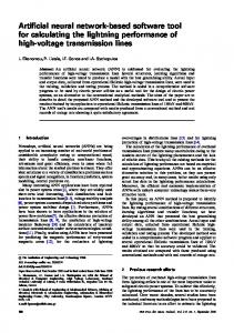
Fig.4 shows the step response of the batch reactor closedloop system using both adaptive FOPID and GPC controllers.
----------------
Fig. 4. Step responses of the closed-loop system of the batch reactor. Circles represent the adaptive FOPID and solid line represents the GPC controller.
As it is shown in Fig. 4, better performance has been achieved using adaptive FOPID controller.
ReicAdtr
H>
ErchaO
2) Tank temperature control: The next example is the temperature control in a tank, which has a typical continuous time transfer function, given by
G(s)
Fig. 3. Schematic diagram of a batch reactor
The sampling time chosen here is TI = 12s, which is the same as the one used in [23]. The GPC parameters are also selected to be:
TI =12s, M =5, P= 7andy =1 where M is the control horizon and P is the prediction horizon. Also -y = 1 shows that, the control effort and the
50+ (0.41e
--s(1 + 50s)
(31)
The manipulated variable in this case is the duty cycle of the heating resistor. The process has integral effect and was identified around the nominal operating condition (500C). The delay of this process is also common in the most chemical processes and cause ordinary controllers to fail in many cases. In the case study presented in here, The GPC parameters are set to be
766
Ts
=
10s, M
=
6, P
=
5 and a
=
1.2
Now, using Ts = 10s and Q = 100, for the proposed adaptive FOPID controller, the following parameters, as shown in table II, have been achieved after learning process. TABLE II ADAPTIVE FOPID PARAMETERS
-0.1078 -1.1492 1.1245 bKp 1.5167 1.2736 bK1 4.4541 bKD KKp 0.0012 -0.0002 0.0002 A -2.3444 0.4985 AI
aKp
aK1 aKD
Fig. 5 shows the output of the system after applying the proposed adaptive FOPID controller and also the GPC.
Fig. 5. Step responses of the closed-loop tank temperature control system.Circles represent the adaptive FOPID and solid line represents the GPC controller.
Using Fig. 5, it can be seen that the purposed controller has a better control performance than the GPC. VII. CONCLUSIONS
In this paper, a new adaptive FOPID controller based on auto-tuning neurons has been presented. The proposed structure and algorithm leads to much better performance than the other conventional schemes, like GPC. Although, for improving the performance of the overall control system, some other appropriate factors could also be added to the cost
REFERENCES [1] M. Axtell and M.E. Bise, "Fractional calculus applications in control systems," in Proc. IEEE National Aerospace and Electronics Conference, New York, USA, pp. 563-566, 1990. [2] N. Engheta, "On fractional calculus and fractional multipoles in electromagnetism," IEEE Trans. Antennas Propagat, vol. 44, pp. 554566, 1996. [3] M. Unser and T. Blu, "Wavelet theory demystified," IEEE Trans. on Signal Processing, vol. 51, pp. 470-483, 2003. [4] I. Podlubny, "Fractional-order systems and PIA D/ controllers," IEEE Trans. Automatic Control, vol. 44, pp. 208-214, 1999. [5] Y. Q. Chen, D. Xue, and H. Dou. "Fractional Calculus and Biomimetic Control," IEEE Int. Conf. on Robotics and Biomimetics (ROBIO 04), Shengyang, China, Aug 2004. [6] Y. Q. Chen and D. Xue, "A comparative introduction of four fractional order controllers," in Proc. of The 4th IEEE World Congress on Intelligent Control and Automation (WCICA02), Shanghai, China, Jun 2002, pp. 3228-3235. [7] Y. Q. Chen, "Fractional order dynamic system control; A historical note and a comparative introduction of four fractional order controllers," Tutorial Workshop on Fractional Order Calculus in Control and Robotics, IEEE International Conference on Decision and Control (IEEE CDC2002), Las Vegas, NE, USA, Dec. 2002. [8] W.K. Ho, K.W. Lim, and W. Xu, "Optimal gain and phase margin tuning for PID controllers," Automatica, vol.34, no.8, pp.1009-1014, 1998. [9] R. Caponetto, L. Fortuna, and D. Porto, "A new tuning strategy for a non integer order PID controller," IFAC2004, Bordeaux, France, 2004. [10] C.A. Monje, B.M. Vinagre, Y.Q. Chen, V. Feliu, P. Lanusse and J. Sabatier, "Proposals for fractional PIA D tuning," The First IFAC Symposium on Fractional Differentiation and its Applications 2004, Bordeaux, France, July 2004. [11] I. Podlubny, L. Dorcak, I. Kostial,"On fractional derivatives,fractional order dynamic systems and PIAD/I controllers," in Proc. of the 36th IEEE CDC, San Diego, CA. [12] Duarte Pedro Mata de Oliveira Valrio, "ninteger v. 2.3 fractional control toolbox for MatLab," UNIVERSIDADE TECNICA DE LISBOA INSTITUTO SUPERIOR TECNICO. [13] G.E. Carlson, C.A. Halijak, "Approximation of fractional capacitors (1ls) 11 by a regular Newton process,"IEEE Transactions on Circuit Theory, pp. 210-213, 1964. [14] M.A. CHADO, J.A. Tenreiro, "Discrete-time fractional-order controllers," Journal of Fractional Calculus and Applied Analysis, pp. 47-66, 2001. [15] K.B. Oldham and J. Spanier,The Fractional Calculus, Academic Press, New York, 1974. [16] Wei-Der Changa, Rey-Chue Hwangb, Jer-Guang Hsieh, "A multivariable on-line adaptive PID controller using auto-tuning neurons," Engineering Applications of Artificial Intelligence, Elsevier Science Ltd., pp. 5763, 2001. [17] MATLAB Optimization Toolbox User's Guide, Mathworks Inc. 2004. [18] C.G. Broyden, "The convergence of a class of double-rank minimization algorithms," J. Inst. Maths. Applics., vol. 6, pp. 76-90, 1970. [19] R. Fletcher, "A new approach to variable metric algorithms," Computer Journal, vol. 13, pp. 317-322, 1970. [20] D. Goldfarb, "A family of variable metric updates derived by variational means," Mathematics of Computing, vol. 24, pp. 23-26, 1970. [21] D.F. Shanno, "Conditioning of quasi-newton methods for function minimization," Mathematics of Computing, vol. 24, pp. 647-656, 1970. [22] R. Schoenberg, "Optimization with the quasi-newton method," Aptech Systems Inc., Maple Valley, WA, Sep. 2001. [23] B. Cott, F. Macchietto, "Temperature control of exothermic batch reactor using generic model control ," Industrial and Engineering Chemistry Research, pp. 1177-1184, 1989.
function. Moreover, the evolutionary algorithms could have been used for optimization purposes instead, which is also under investigation by the authors.
767