A New Neural Network for Solving Nonlinear Programming Problems

A New Neural Network for Solving Nonlinear Programming Problems Yun Gao, Xianyun Xu, and Yongqing Yang School of Science, Jiangnan University, Wuxi 214122, PR China

Abstract. In this paper a new neural network is proposed to solve nonlinear convex programming problems. The proposed neural network is shown to be asymptotically stable in the sense of Lyapunov. Comparing with the existing neural networks, the proposed neural network has fewer state variables and simpler architecture. Numerical examples show that the proposed network is feasible and efficient. Keywords: asymptotical stability, neural network, nonlinear programming.

1

Introduction

Nonlinear programming problems are commonly encountered in modern science and technology, such as optimal control, signal processing, pattern recognition[1]. In many engineering applications, the real-time solution of optimization problems is required. However, traditional algorithms may not be efficient since the computing time required for a solution is greatly dependent on the dimension and structure of the problems. One possible and very promising approach to real-time optimization is to apply artificial neural networks[2, 3]. In 1985 Tank and Hopfield first proposed the neural network for linear programming problems [4]. Their work has inspired many researchers to investigate other neural network models for solving programming problems. Over the years, neural network models have been developed to solve nonlinear programming problems. Kennedy and Chua [5] presented a neural network for solving nonlinear programming problems. It is known that the neural network model contains finite penalty parameters and generates approximate solutions only. To avoid using penalty parameters, many other methods have been done in recent years. Zhang and Constantinides developed [6] a Lagrange neural network for a nonlinear programming problem with equality constrains. Xia [7] presented some primal neural networks for solving convex quadratic programming problems and nonlinear convex optimization problems with limit constraints. In order to simplify the architecture of the dual neural network, a simplified dual neural network was introduced for solving convex quadratic programming problems [8]. Leung[9] and Yang[10]presented a feedback neural network for solving convex nonlinear programming problems. Based on the idea of successive approximation, the equilibrium point sequence of subnetworks can converge to an exact optimal solution. D. Liu et al. (Eds.): ISNN 2011, Part I, LNCS 6675, pp. 565–571, 2011. c Springer-Verlag Berlin Heidelberg 2011

566

Y. Gao, X. Xu, and Y. Yang

In [11, 12], Liu and Wang proposed some one-layer recurrent neural networks for solving linear and quadratic programming problems. The one-layer recurrent neural networks have more simply architecture complexity than the other neural networks such as Lagrangian network and projection network. Recently, several projection neural networks were developed for solving general nonlinear convex programming problems [13–21], which were globally convergent to exact optimal solutions. In this paper, we present a new neural network for solving nonlinear programming problems. The proposed neural network is asymptotically stable in the sense of Lyapunov. Compared with existing neural networks for such problems, the proposed neural network has fewer state variables, simpler architecture and weaker convergence conditions. This paper is divided into 5 sections. In section 2, the nonlinear convex programming problem is described. A new neural network model is proposed to solve this problem. In section 3, we prove the stability of the proposed neural network. Two examples are provided to show the effectiveness of the proposed neural network in section 4. Finally, some conclusions are found in section 5.

2

Problem and the Neural Network Model

In this section,we describe the nonlinear convex programming problem and its equivalent formulation. Then we construct a new neural network for solving this problem. Consider the following nonlinear convex programming problem: min f (x) subject to Ax = b g(x) ≥ 0.

(1)

where x = (x1 , x2 , · · · , xn )T ∈ Rn , g(x) = (g1 (x), g2 (x), · · · , gp (x))T ∈ Rp , f (x), −gi (x) (i = 1, 2, · · · , p) are continuously differentiable and convex form Rn to R, A ∈ Rm×n , and rank(A) = m (0 < m < n), b ∈ Rm . According to the Karash-Kuhn-Tucker (KKT ) conditions for convex optimization [1], the following set of equations has the same solutions as the problem(1). (2) ∇f (x) + AT λ − g (x)T y = 0 Ax = b

(3)

g(x) ≥ 0, y ≥ 0, y g(x) = 0 T

(4)

From(2) and (3), we have [I − AT (AAT )−1 A][∇f (x) − g (x)T y] + AT (AAT )−1 (Ax − b) = 0 Let P = AT (AAT )−1 A, then the above equation can be written as (I − P )[∇f (x) − g (x)T y] + P x − Q = 0 where Q = AT (AAT )−1 b.

(5)

A New Neural Network for Nonlinear Programming

567

By the projection theorem , (4) is equivalent to solving the following equation: (y − g(x))+ − y = 0

(6)

where (y)+ = ([y1 ]+ , · · · , [yn ]+ )T , [yi ]+ = max{0, yi }. Based on (5) and (6), we propose a neural network for solving (1) as follows: dx dt dy dt

= −2{(I − P )[∇f (x) − g (x)T (y − g(x))+ ] − P x + Q} = −y + (y − g(x))+

(7)

Remark 1. From above analysis, it is obvious that x∗ is an optimal solution of (1) if and only if (x∗ , y ∗ )T is an equilibrium point of system (7). Remark 2. Comparing with the existing neural networks for solving problem (1). It is easy to see the neural network in [19], has n + m + p state variables. However, our neural network has only n + p state variables. Remark 3. In [16, 17], Xia proposed recurrent neural networks for nonlinear convex optimization subject to linear or nonlinear constraints. Under the conditions that f (x) or gi (x) are assumed to be strictly convex, the convergence of the proposed neural network are obtained. However, our neural network can converge to the optimal solution if only f (x) and −gi (x) are convex.

3

Stability Analysis

In this section, we prove the global asymptotical stability of the neural network(7). Lemma 1. Assume f (x) and −gi (x) are convex. Let (x∗ , y ∗ ) be an equilibrium point of neural network (7) and ϕ(x, y) = f (x) + 12 (y − g(x))+ 2 , then (I) ϕ(x, y) is a differential convex function and ∇f (x) − g (x)T (y − g(x))+ ∇ϕ(x, y) = (y − g(x))+ (II) ϕ(x, y) − ϕ(x∗ , y ∗ ) − (x − x∗ )T (∇f (x∗ ) − g (x∗ )T y ∗ ) − (y − y ∗ )T y ∗ ≥ 0. The proof of this Lemma is easy and we omit it. Theorem 1. The neural network (7) is asymptotically stable in the sense of Lyapunov for any initial point (x(t0 ), y(t0 )) ∈ Rn+p . Proof. Let (x∗ , y ∗ )T be an equilibrium of (7), considering the following Lynapov function V (x, y) = ϕ(x, y) − ϕ(x∗ , y ∗ ) − (x − x∗ )T ∇ϕx (x∗ , y ∗ ) − (y − y ∗ )T ∇ϕy (x∗ , y ∗ ) 1 1 + x − x∗ 2 + y − y ∗ 2 2 2

568


By Lemma 1, we can obtain the following inequality 1 1 V (x, y) ≥ x − x∗ 2 + y − y ∗ 2 . 2 2 Calculating the derivative of V along the solution of (7), dV dt

(8)

∂V dy dx = ∂V ∂x dt + ∂y dt = −2[∇f (x) − g (x)T (y − g(x))+ − ∇f (x∗ ) + g (x∗ )T y ∗ + x − x∗ ]T {(I − P )[∇f (x) − g (x)T (y − g(x))+ ] − P x + Q} −[y − (y − g(x))+ ]T [(y − g(x))+ − 2y ∗ + y] = −[∇f (x) − ∇f (x∗ ) + x − x∗ + g (x∗ )T y ∗ − g (x)T (y − g(x))+ ]T {(I − P )[∇f (x) − ∇f (x∗ )] + (I − P )[g (x∗ )T y ∗ − g (x)T (y − g(x))+ ] +P (x − x∗ )} −[y −(y − g(x))+ ]T [y − (y − g(x))+ + 2(y − g(x))+ − 2y ∗ ]

= −2 [∇f (x) − ∇f (x∗ )]T (I − P )[∇f (x) − ∇f (x∗ )] +[∇f (x) − ∇f (x∗ )]T (I − P )[g (x∗ )T y ∗ − g (x)T (y − g(x))+ ] +[∇f (x) − ∇f (x∗ )]T P (x − x∗ ) +(x − x∗ )T (I − P )[∇f (x) − ∇f (x∗ )] +(x − x∗ )T (I − P )[g (x∗ )T y ∗ − g (x)T (y − g(x))+ ] +(x − x∗ )T P (x − x∗ ) +[g (x∗ )T y ∗ − g (x)T (y − g(x))+ ]T (I − P )[∇f (x) − ∇f (x∗ )] ∗ T ∗ T + +[g (x∗ )T y ∗ − g (x)T (y − g(x))+ ]T (I − P )[g (x ) y − g (x) (y − g(x)) ]

+[g (x∗ )T y ∗ − g (x)T (y − g(x))+ ]T P (x − x∗ ) − y − (y − g(x))+ 2 −2[y − (y − g(x))+ ]T [(y − g(x))+ − y ∗ ]

Noting that (I − P )2 = I − P , P 2 = P and P (I − P ) = 0, we have dV ∗ T 2 ∗ dt = −2 [∇f (x) − ∇f (x )] (I − P ) [∇f (x) − ∇f (x )] +2[∇f (x) − ∇f (x∗ )]T (I − P )2 [g (x∗ )T y ∗ − g (x)T (y − g(x))+ ] +[g (x∗ )T y ∗ − g (x)T (y− g(x))+ ]T (I − P )2 [g (x∗ )T y ∗ − g (x)T (y − g(x))+ ]

+(x − x∗ )T P 2 (x − x∗ ) − 2(x − x∗ )T [∇f (x) − ∇f (x∗ )] −2(x − x∗ )T [g (x∗ )T y ∗ − g (x)T (y − g(x))+ ] − y − (y − g(x))+ 2 −2[g(x) − (g(x) − y)+ ]T [(y − g(x))+ − y ∗ ] = −2 (I − P )[∇f (x) − ∇f (x∗ )] + (I − P )[g (x∗ )T y ∗ − g (x)T (y − g(x))+ ] +P (x − x∗ ) 2 −2(x − x∗ )T [∇f (x) − ∇f (x∗ )] − 2(x − x∗ )T g (x∗ )T y ∗ −2(x − x∗ )T g (x)T (y − g(x))+ − y − (y − g(x))+ 2 −2g(x)T (y − g(x))+ + 2g(x)T y ∗ −2[(g(x) − y))+ ]T (y − g(x))+ − 2[(y − g(x))+ ]T y ∗ = −2 (I − P )[∇f (x) − g (x)T (y − g(x))+ ] − P x + Q 2 − y − (y − g(x))+ 2 −2(x − x∗ )T [∇f (x) − ∇f (x∗ )] − [(y − g(x))+ ]T y ∗ −2(x − x∗ )T g (x∗ )T y ∗ − 2(x − x∗ )T g (x)T (y − g(x))+ − 2g(x)T (y − g(x))+ +g(x)T y ∗ = −2 (I − P )[∇f (x) − g (x)T (y − g(x))+ ] − P x + Q 2 − y − (y − g(x))+ 2 −2(x − x∗ )T [∇f (x) − ∇f (x∗ )] − [(y − g(x))+ ]T y ∗ +2[g(x) − g(x∗ ) − g (x∗ )(x − x∗ )]T y ∗ + g(x∗ )T y ∗ +2[g(x∗ ) − g(x) − g (x)(x∗ − x)]T (y − g(x))+ − 2g(x∗ )T (y − g(x))+


569

Since f (x) and −gi (x) are convex function, we have (x − x∗ )T [∇f (x) − ∇f (x∗ )] ≥ 0 g(x∗ ) − g(x) − g(x)(x∗ − x) ≤ 0 g(x) − g(x∗ ) − g(x∗ )(x − x∗ ) ≤ 0

(9)

In addition, it is easy to verify [(g(x) − y)+ ]T (y − g(x))+ = 0, g(x∗ )T y ∗ = 0, and [(g(x) − y)+ ]T y ∗ ≥ 0, g(x∗ )T [y − (g(x))+ ]T ≥ 0. Thus, dV dt

≤ −2 (I − P )[∇f (x) − g (x)T (y − g(x))+ ] − P x + Q 2 − y − (y − g(x))+ 2 < 0, ∀ (x, y) = (x∗ , y ∗ ).

(10)

Thus, the neural network is asymptotically stable for any initial points. This completes the proof.

4

Numerical Examples

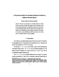
In this section, we will give two examples to demonstrate the effectiveness of the proposed neural network. Example 1. Consider the following nonlinear programming problem. minimize subject to

f (x) = x41 + (x2 − 2)2 + (x2 − x3 )2 3x1 − x2 + 4x3 = 6 −x1 + 2x2 + 3x3 = 10 g1 (x) = x21 + x22 + x23 − 8 ≤ 0 g2 (x) = 2x21 + 2x22 + x23 − 12 ≤ 0

This problem has an optimal solution x∗ = (0, 2, 2)T . The simulation result shows the neural network (7) converges to the optimal solution. The Fig. 1 is the state trajectory of neural network (7). 3 2 1 0 −1 −2 −3 −4 −5

0

10

20

30

40

50

Fig. 1. Transient behavior of (7) in Example 1

570


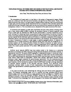
Example 2. Consider the following nonlinear programming problem. minimize subject to

f (x) = (x1 − 1)4 + (x1 − 2x2 )4 + (4x2 − x3 )4 + (x4 − x5 )4 2x3 − x4 + x5 = 4 −x1 + 2x2 + 2x3 + x4 + x5 = 4 g1 (x) = x21 + x23 + x24 − 5 ≤ 0 g2 (x) = x21 + 4x22 + 4x25 − 3 ≤ 0

This problem has an optimal solution x∗ = (1, 0.5, 2, 0, 0)T . The simulation result shows the neural network (7) converges to the optimal solution. The Fig. 2 is the state trajectory of neural network (7). 3

2

1

0

−1

−2

−3

−4

0

10

20

30

40

50

Fig. 2. Transient behavior of (7) in Example 2

5

Conclusion

In this paper, we present a new neural network for solving nonlinear convex programming problems. The proposed neural network is asymptotically stable in sense of Lyapunov. Comparing with other neural networks for nonlinear convex optimization, the proposed neural network has fewer neurons and simpler architecture. Some examples are given to illustrate the effectiveness of the proposed neural network.

Acknowledgement This work was jointly supported by the National Natural Science Foundation of China under Grant 60875036, the Key Research Foundation of Science and Technology of the Ministry of Education of China under Grant 108067, and supported by Program for Innovative Research Team of Jiangnan University.

References 1. Bazaraa, M., Sherali, H., Shetty, C.: Nonlinear programming: Theory and algorithms. Wiley, New York (1993) 2. Hopfield, J., Tank, D.: Neural computation of decisions in optimization problem. Biol. Cybern. 52, 141–152 (1985)


571

3. Cichocki, A., Unbehauen, R.: Neural networks for optimization and signal processing. Wiley, New York (1993) 4. Tank, D., Hopfield, J.: Simple neural optimization networks: an A/D converter, signal decision circuit. IEEE Trans. Cir. Sys. 33(5), 533–541 (1986) 5. Kennedy, M., Chua, L.: Neural network for nonlinear programming. IEEE Trans. Cir. Sys. 35(5), 554–562 (1988) 6. Zhang, S., Constantinides, A.: Lagrange programming neural networks. IEEE Trans. Cir. Sys. 39(7), 441–452 (1992) 7. Xia, Y.: A new neural network for solving linear and quadratic programming problems. IEEE Trans. Neural. Net. 7(6), 1544–1547 (1996) 8. Liu, S., Wang, J.: A simplified dual neural network for quadratic programming with its KWTA application. IEEE Trans. Neu. Net. 17(6), 1500–1510 (2006) 9. Leung, Y., Gao, X.: A high-performance feedback neural network for solving convex nonlinear programming problems. IEEE Trans. Neu. Net. 14, 1469–1477 (2003) 10. Yang, Y., Cao, J.: A feedback neural network for solving convex constraint optimization problems. App. Mathe. Compu. 201(1-2), 340–350 (2008) 11. Liu, Q., Wang, J.: A one-layer recurrent neural network with a discontinuous activation function for linear programming. Neur. Compu. 20(5), 1366–1383 (2008) 12. Liu, Q., Wang, J.: A one-layer recurrent neural network with a discontinuous hardlimiting activation function for quadratic programming. IEEE Trans. Neu. Net. 19(4), 558–570 (2008) 13. Tao, Q., Cao, J., Xue, M., Qiao, H.: A high performance neural network for solving nonlinear programming problems with hybrid constraints. Phys. Let. A 288, 88–94 (2001) 14. Effati, S., Baymani, M.: A new nonlinear neural network for solving quadratic programming problems. Appl. Mathe. Compu. 165, 719–729 (2005) 15. Xia, Y., Leung, H., Wang, J.: A projection neural network and its application to constrained optimization problems. IEEE Trans. Cir. Sys. 49(4), 447–458 (2002) 16. Xia, Y., Wang, J.: A recurrent neural network for nonlinear convex optimization subject to nonlinear inequality constraints. IEEE Trans. Cir. Sys. 51(7), 1385–1394 (2004) 17. Xia, Y., Wang, J.: A recurrent neural network for nonlinear convex optimization subject to linear constraints. IEEE Trans. Cir. Sys. 16(2), 379–386 (2005) 18. Liang, X.: A recurrent neural networks for nonlinear continuously differentiable optimization over a compact convex subset. IEEE Trans. Neur. Net. 12, 1487–1490 (2001) 19. Gao, X.: A novel neural network for nonlinear convex programming. IEEE Trans. Neu. Net. 15, 613–621 (2004) 20. Hu, X., Wang, J.: Solving pseudomonotone variational inequalities and pseudoconvex optimization problems using the projection neural network. IEEE Trans. Neu. Net. 17(6), 1487–1499 (2006) 21. Hu, X.: Applications of the general projection neural network in solving extended linear-quadratic programming problems with linear constraints. Neurocom. 72, 1131–1137 (2009) 22. Avriel, M.: Nonlinear programming: Analysis and Methods. Prentice-Hall, Englewood Cliffs (1976) 23. Miller, R., Michel, A.: Ordinary differential equations. Academic, New York (1982)