A Note on the Implementation of Hierarchical Dirichlet Processes
Recommend Documents
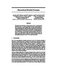
We propose the hierarchical Dirichlet process (HDP), a nonparametric. Bayesian model for clustering problems involving multiple groups of data. Each group of ...
Jul 28, 2010 - may first appear in blogs, and then spread to news and message boards. Fig. .... To the best of our knowledge, there are four works that seem- ingly involve ...... We follow the dependencies of different sets of variables and ...
restaurant process that we refer to as the âChinese restaurant franchise. .... where the Ïk are independent random variables distributed ac- cording to G0, where ...
detection of abnormal behaviours that in isolation appear normal. Pragmatic ... ing behaviour temporally, which models which behaviours occur together, and ...
Mar 24, 2009 - We prove an asymptotic formula for the fourth power mean of Dirichlet ... puting the fourth moment for prime moduli q with a power saving in the ...
A gentle tutorial ... Dirichlet distribution, and Dirichlet Process introduction ..... ―A
Bayesian Analysis of Some Nonparametric Problems‖ Annals of Statistics.
the case of the generalized Dirichlet distribution thanks to some interesting mathematical ..... Batch variational inference for the proposed model ...... This paper has presented a unified framework for simultaneous clustering and ..... [2] Heusch G
or topic mixtures. Making use of a nested Chinese Restaurant Franchise ..... Inner restaurants are assigned to the tables of each outer restaurant ac- cording to ...
convergence on PX, the wellâknown de Finetti representation theorem leads to a mixture representation ...... Indeed, they are the key for devising Blackwell-MacQueen type al- gorithms for ..... MR2197664. [26] Rao, V.A. and Teh, Y.W. (2009).
Sep 17, 2015 - 4 Inference by Gibbs Sampling ... Next we describe a Gibbs sampler for the DFP. .... Cor J. Veenman, Marcel J. T. Reinders, and Eric Backer.
May 12, 2014 - HDSP uses the distances between labels and top- ics to scale the topic proportions such that the topics closer to the observed labels in a document ..... complex metric learning problems (Xing et al., 2002) or the kernel based ...
For a given weakly convergent sequence fX ng of Dirichlet processes we show weak convergence of the sequence of the corresponding quadratic variation ...
We exhibit a trigonometric identity wich implies a link between the kernels of ... has to be restricted to a definite class of functions f(y) verifying the known Dirichlet.
Apr 19, 2010 - t is the Ï-algebra generated by the history X0,..., Xt. If the initial distribution ..... 2nd Edition, Cambridge University Press, Cambridge. [7] Pollard ...
Roberts (2008) and Walker (2007) for Dirichlet mixture models are ... Walker (2007) makes the neat observation that, in the spirit of slice sampling, rather.
Mar 15, 2014 - X =Ï#(A)P# + P#API + PIAP# + PIAPI + aPN\I , ... [3] Ben Ghorbal A. Schurmann M. Quantum stochastic calculus on Boolean Fock space, Infin.
Giulio Trichilo. Department of Artificial Intelligence (E3) Jozef Stefan Institute, Ljubljana. [Internship] ..... 1, the restaurants referred to on its table's cards are at level 2, and so on. [7]. Department of Artificial ..... _____,i ____ ........
Sep 22, 2011 - FEDERICO BASSETTI, ROBERTO CASARIN, AND FABRIZIO LEISEN. Abstract. Time series data may exhibit clustering over time and, in a ...
Computer Science Department, Indiana University ... [email protected]. Abstract ... Each newly allocated node in javar is linked in a list using the eld.
clauses. We describe these features and their. 1Linear logic is an important example of the family of relevance logics 12]. 2This name is not acronym; its origin is.
Depts. of Neurology and Bioengineering, University of Pennsylvania, ... a patient hasâ and âwhich other patients is this pa- ...... Springer-Verlag, Berlin, 2006.
Bayesian non parametric extension of the classical Hidden Markov Model (HMM)
... (HMMs) [1] have been applied for learning and recognition of time-series.
Springer International Publishing AG, part of Springer Nature 2018 ... Manual segmentation is time consuming and not possible for a large acoustic ..... demo: http://sabiod.univ-tln.fr/workspace/MTAP/bird.zip. .... a tutorial review and prospectus.
ing algorithms PCM and PCQ, by incorporating the tempo- ral smoothness to ..... [24] to quantitatively compare the clustering performances among all the four ...
A Note on the Implementation of Hierarchical Dirichlet Processes
Department of Informatics University of Edinburgh Edinburgh, EH8 9AB, UK
†
Department of Cognitive and Linguistic Sciences Brown University Providence, RI, USA
Abstract
correction, the approximation is poor for hierarchical models, which are commonly used for NLP applications. We derive an improved O(1) formula that gives exact values for the expected counts in non-hierarchical models. For hierarchical models, where our formula is not exact, we present an efficient method for sampling from the HDP (and related models, such as the hierarchical PitmanYor process) that considerably decreases the memory footprint of such models as compared to the naive implementation. As we have noted, the issues described in this paper apply to models for various kinds of NLP tasks; for concreteness, we will focus on n-gram language modeling for the remainder of the paper, closely following the presentation in GGJ06.
The implementation of collapsed Gibbs samplers for non-parametric Bayesian models is non-trivial, requiring considerable book-keeping. Goldwater et al. (2006a) presented an approximation which significantly reduces the storage and computation overhead, but we show here that their formulation was incorrect and, even after correction, is grossly inaccurate. We present an alternative formulation which is exact and can be computed easily. However this approach does not work for hierarchical models, for which case we present an efficient data structure which has a better space complexity than the naive approach.
1
2
Introduction
The Chinese Restaurant Process
GGJ06 present two nonparametric Bayesian language models: a DP unigram model and an HDP bigram model. Under the DP model, words in a corpus w = w1 . . . wn are generated as follows:
Unsupervised learning of natural language is one of the most challenging areas in NLP. Recently, methods from nonparametric Bayesian statistics have been gaining popularity as a way to approach unsupervised learning for a variety of tasks, including language modeling, word and morpheme segmentation, parsing, and machine translation (Teh et al., 2006; Goldwater et al., 2006a; Goldwater et al., 2006b; Liang et al., 2007; Finkel et al., 2007; DeNero et al., 2008). These models are often based on the Dirichlet process (DP) (Ferguson, 1973) or hierarchical Dirichlet process (HDP) (Teh et al., 2006), with Gibbs sampling as a method of inference. Exact implementation of such sampling methods requires considerable bookkeeping of various counts, which motivated Goldwater et al. (2006a) (henceforth, GGJ06) to develop an approximation using expected counts. However, we show here that their approximation is flawed in two respects: 1) It omits an important factor in the expectation, and 2) Even after
G|α0 , P0 wi |G
∼ DP(α0 , P0 ) ∼G
where G is a distribution over an infinite set of possible words, P0 (the base distribution of the DP) determines the probability that an item will be in the support of G, and α0 (the concentration parameter) determines the variance of G. One way of understanding the predictions that the DP model makes is through the Chinese restaurant process (CRP) (Aldous, 1985). In the CRP, customers (word tokens wi ) enter a restaurant with an infinite number of tables and choose a seat. The table chosen by the ith customer, zi , follows the distribution: ( z nk−i i−1+α0 , 0 ≤ k < K(z−i ) P (zi = k|z−i ) = α0 i−1+α0 , k = K(z−i ) 337
Proceedings of the ACL-IJCNLP 2009 Conference Short Papers, pages 337–340, c Suntec, Singapore, 4 August 2009. 2009 ACL and AFNLP
a
b
c
d
e
f
The
cats
cats
1
2
3
h
meow 4
g
Expectation Antoniak approx. Empirical, fixed base Empirical, inferred base
cats 5
100
Mean number of lexical entries
Figure 1. A seating assignment describing the state of a unigram CRP. Letters and numbers uniquely identify customers and tables. Note that multiple tables may share a label.
where z−i = z1 . . . zi−1 are the table assignments z of the previous customers, nk−i is the number of customers at table k in z−i , and K(z−i ) is the total number of occupied tables. If we further assume that table k is labeled with a word type `k drawn from P0 , then the assignment of tokens to tables defines a distribution over words, with wi = `zi . See Figure 1 for an example seating arrangement. Using this model, the predictive probability of wi , conditioned on the previous words, can be found by summing over possible seating assignments for wi , and is given by
10
1
0.1 1
10 100 Word frequency (nw)
1000
Figure 2. Comparison of several methods of approximating the number of tables occupied by words of different frequencies. For each method, results using α = {100, 1000, 10000, 100000} are shown (from bottom to top). Solid lines show the expected number of tables, computed using (3) and assuming P1 is a fixed uniform distribution over a finite vocabulary (values computed using the Digamma formulation (7) are the same). Dashed lines show the values given by the Antoniak approximation (4) (the line for α = 100 falls below the bottom of the graph). Stars show the mean of empirical table counts as computed over 1000 samples from an MCMC sampler in which P1 is a fixed uniform distribution, as in the unigram LM. Circles show the mean of empirical table counts when P1 is inferred, as in the bigram LM. Standard errors in both cases are no larger than the marker size. All plots are based on the 30114word vocabulary and frequencies found in sections 0-20 of the WSJ corpus.
w
nw −i + α0 P0 P (wi = w|w−i ) = (1) i − 1 + α0 This prediction turns out to be exactly that of the DP model after integrating out the distribution G. Note that as long as the base distribution P0 is fixed, predictions do not depend on the seating arrangement z−i , only on the count of word w w in the previously observed words (nw −i ). However, in many situations, we may wish to estimate the base distribution itself, creating a hierarchical model. Since the base distribution generates table labels, estimates of this distribution are based on the counts of those labels, i.e., the number of tables associated with each word type. An example of such a hierarchical model is the HDP bigram model of GGJ06, in which each word type w is associated with its own restaurant, where customers in that restaurant correspond to words that follow w in the corpus. All the bigram restaurants share a common base distribution P1 over unigrams, which must be inferred. Predictions in this model are as follows:
these kinds of models, the counts are constantly changing over multiple samples, with tables going in and out of existence frequently. This can create significant bookkeeping issues in implementation, and motivated GGJ06 to present a method of computing approximate table counts based on word frequencies only.
h
P2 (wi |h−i ) =
n(w−ii−1 ,wi ) + α1 P1 (wi |h−i )
3
h
n(w−ii−1 ,∗) + α1
Approximating Table Counts
h
P1 (wi |h−i ) =
tw−i i + α0 P0 (wi ) h
t∗ −i + α0
(2)
Rather than explicitly tracking the number of tables tw associated with each word w in their bigram model, GGJ06 approximate the table counts using the expectation E[tw ]. Expected h h counts are used in place of tw−i and t∗ −i in (2). i The exact expectation, due to Antoniak (1974), is nw X 1 E[tw ] = α1 P1 (w) (3) α1 P1 (w) + i − 1
h
where h−i = (w−i , z−i ), tw−i is the number of i h tables labelled with wi , and t∗ −i is the total number of occupied tables. Of particular note for our discussion is that in order to calculate these conditional distributions we must know the table assignments z−i for each of the words in w−i . Moreover, in the Gibbs samplers often used for inference in
i=1
338
Explicit table tracking: customer(w i ) → table(zi ) n
Antoniak also gives an approximation to this expectation:
a : 1, b : 1, c : 2, d : 2, e : 3, f : 4, g : 5, h : 5
nw + α1 P1 (w) E[tw ] ≈ α1 P1 (w) log (4) α1 P1 (w) but provides no derivation. Due to a misinterpretation of Antoniak (1974), GGJ06 use an approximation that leaves out all the P1 (w) terms from (4).1 Figure 2 compares the approximation to the exact expectation when the base distribution is fixed. The approximation is fairly good when αP1 (w) > 1 (the scenario assumed by Antoniak); however, in most NLP applications, αP1 (w) < 1 in order to effect a sparse prior. (We return to the case of non-fixed based distributions in a moment.) As an extreme case of the paucity of this approximation consider α1 P1 (w) = 1 and nw = 1 (i.e. only one customer has entered the restaurant): clearly E[tw ] should equal 1, but the approximation gives log(2). We now provide a derivation for (4), which will allow us to obtain an O(1) formula for the expectation in (3). First, we rewrite the summation in (3) as a difference of fractional harmonic numbers:2 H(α1 P1 (w)+nw −1) − H(α1 P1 (w)−1)
table(zi ) → label(`) n o 1 : T he, 2 : cats, 3 : cats, 4 : meow, 5 : cats Histogram: n o word type → table occupancy → frequency n
T he : {2 : 1}, cats : {1 : 1, 2 : 2}, meow : {1 : 1}
o
Figure 3. The explicit table tracking and histogram representations for Figure 1.
(5)
Using the recurrence for harmonic numbers: h 1 E[tw ] ≈ α1 P1 (w) H(α1 P1 (w)+nw ) − α1 P1 (w) + nw i 1 (6) − H(α1 P1 (w)+nw ) + α1 P1 (w) We then use the asymptotic expansion, 1 HF ≈ log F + γ + 2F , omiting trailing terms −2 which are O(F ) and smaller powers of F :3 1 P1 (w) E[tw ] ≈ α1 P1 (w) log nwα+α + 1 P1 (w)
o
nw 2(α1 P1 (w)+nw )
Omitting the trailing term leads to the approximation in Antoniak (1974). However, we can obtain an exact formula for the expectation by utilising the relationship between the Digamma function and the harmonic numbers: ψ(n) = Hn−1 − γ.4 Thus we can rewrite (5) as:5
A significant caveat here is that the expected table counts given by (3) and (7) are only valid when the base distribution is a constant. However, in hierarchical models such as GGJ06’s bigram model and HDP models, the base distribution is not constant and instead must be inferred. As can be seen in Figure 2, table counts can diverge considerably from the expectations based on fixed P1 when P1 is in fact not fixed. Thus, (7) can be viewed as an approximation in this case, but not necessarily an accurate one. Since knowing the table counts is only necessary for inference in hierarchical models, but the table counts cannot be approximated well by any of the formulas presented here, we must conclude that the best inference method is still to keep track of the actual table counts. The naive method of doing so is to store which table each customer in the restaurant is seated at, incrementing and decrementing these counts as needed during the sampling process. In the following section, we describe an alternative method that reduces the amount of memory necessary for implementing HDPs. This method is also appropriate for hierarchical Pitman-Yor processes, for which no closed-form approximations to the table counts have been proposed.
4
Efficient Implementation of HDPs
As we do not have an efficient expected table count approximation for hierarchical models we could fall back to explicitly tracking which table each customer that enters the restaurant sits at. However, here we describe a more compact representation for the state of the restaurant that doesn’t require explicit table tracking.6 Instead we maintain a histogram for each dish wi of the frequency of a table having a particular number of customers. Figure 3 depicts the histogram and explicit representations for the CRP state in Figure 1. Our alternative method of inference for hierarchical Bayesian models takes advantage of their
The authors of GGJ06 realized this error, and current implementations of their models no longer use these approximations, instead tracking table counts explicitly. 2 Fractional harmonic numbers between 0 and 1 are given R1 F by HF = 0 1−x dx. All harmonic numbers follow the 1−x recurrence HF = HF −1 + F1 . 3 Here, γ is the Euler-Mascheroni constant. 4 Accurate O(1) approximations of the Digamma function are readily available. 5 (7) can be derived from (3) using: ψ(x+1)−ψ(x) = x1 .
6 Teh et al. (2006) also note that the exact table assignments for customers are not required for prediction.
339
5
Algorithm 1 A new customer enters the restaurant 1: 2: 3: 4:
w: word type P0w : Base probability for w HDw : Seating Histogram for w procedure INCREMENT(w, P0w , HDw ) w nw −1 w−1 nw +α0 α0 ×P0w w−1 nw +α0
5:
pshare ←
6:
pnew ←
7: 8: 9: 10:
We’ve shown that the HDP approximation presented in GGJ06 contained errors and inappropriate assumptions such that it significantly diverges from the true expectations for the most common scenarios encountered in NLP. As such we emphasise that that formulation should not be used. Although (7) allows E[tw ] to be calculated exactly for constant base distributions, for hierarchical models this is not valid and no accurate calculation of the expectations has been proposed. As a remedy we’ve presented an algorithm that efficiently implements the true HDP without the need for explicitly tracking customer to table assignments, while remaining simple to implement.
. share an existing table . open a new table
r ← random(0, pshare + pnew ) w if r < pnew or nw −1 = 0 then HDw [1] = HDw [1] + 1 else . Sample from the histogram of customers at tables w r ← random(0, nw −1 ) for c ∈ HDw do . c: customer count r = r − (c × HDw [c]) if r ≤ 0 then HDw [c] = HDw [c] + 1 Break w−1 w nw = nw + 1 . Update token count
11: 12: 13: 14: 15: 16: 17:
Acknowledgements
Algorithm 2 A customer leaves the restaurant 1: w: word type 2: HDw : Seating histogram for w 3: procedure DECREMENT(w, P0w , HDw ) 4: r ← random(0, nw w) 5: for c ∈ HDw do . c: customer count 6: r = r − (c × HDw [c]) 7: if r ≤ 0 then 8: HDw [c] = HDw [c] − 1 9: if c > 1 then 10: HDw [c − 1] = HDw [c − 1] + 1 11: Break w 12: nw . Update token count w = nw − 1
The authors would like to thank Tom Griffiths for providing the code used to produce Figure 2 and acknowledge the support of the EPSRC (Blunsom, grant EP/D074959/1; Cohn, grant GR/T04557/01).
References D. Aldous. 1985. Exchangeability and related topics. In ´ ´ e de Probabiliti´es de Saint-Flour XIII 1983, 1– Ecole d’Et´ 198. Springer.
exchangeability, which makes it unnecessary to know exactly which table each customer is seated at. The only important information is how many tables exist with different numbers of customers, and what their labels are. We simply maintain a histogram for each word type w, which stores, for each number of customers m, the number of tables labeled with w that have m customers. Figure 3 depicts the explicit representation and histogram for the CRP state in Figure 1.
C. E. Antoniak. 1974. Mixtures of dirichlet processes with applications to bayesian nonparametric problems. The Annals of Statistics, 2(6):1152–1174. J. DeNero, A. Bouchard-Cˆot´e, D. Klein. 2008. Sampling alignment structure under a Bayesian translation model. In Proceedings of the 2008 Conference on Empirical Methods in Natural Language Processing, 314–323, Honolulu, Hawaii. Association for Computational Linguistics. S. Ferguson. 1973. A Bayesian analysis of some nonparametric problems. Annals of Statistics, 1:209–230. J. R. Finkel, T. Grenager, C. D. Manning. 2007. The infinite tree. In Proc. of the 45th Annual Meeting of the ACL (ACL-2007), Prague, Czech Republic.
Algorithms 1 and 2 describe the two operations required to maintain the state of a CRP.7 When a customer enters the restaurant (Alogrithm 1)), we sample whether or not to open a new table. If not, we sample an old table proportional to the counts of how many customers are seated there and update the histogram. When a customer leaves the restaurant (Algorithm 2), we decrement one of the tables at random according to the number of customers seated there. By exchangeability, it doesn’t actually matter which table the customer was “really” sitting at.
7
Conclusion
S. Goldwater, T. Griffiths, M. Johnson. 2006a. Contextual dependencies in unsupervised word segmentation. In Proc. of the 44th Annual Meeting of the ACL and 21st International Conference on Computational Linguistics (COLING/ACL-2006), Sydney. S. Goldwater, T. Griffiths, M. Johnson. 2006b. Interpolating between types and tokens by estimating power-law generators. In Y. Weiss, B. Sch¨olkopf, J. Platt, eds., Advances in Neural Information Processing Systems 18, 459–466. MIT Press, Cambridge, MA. P. Liang, S. Petrov, M. Jordan, D. Klein. 2007. The infinite PCFG using hierarchical Dirichlet processes. In Proc. of the 2007 Conference on Empirical Methods in Natural Language Processing (EMNLP-2007), 688–697, Prague, Czech Republic. Y. W. Teh, M. I. Jordan, M. J. Beal, D. M. Blei. 2006. Hierarchical Dirichlet processes. Journal of the American Statistical Association, 101(476):1566–1581.
A
C++ template class that implements the algorithm presented is made available at: http://homepages.inf.ed.ac.uk/tcohn/