A Novel algorithm for Blind Source Separation Based ...

(IJEECS) International Journal of Electrical, Electronics and Computer Systems. Vol: 13 Issue: 02, 2013

A Novel algorithm for Blind Source Separation Based on Fast Nonlinear Autocorrelation Function and Discrete Wavelet Transform Niloufar Rajabiyoun1, Behzad Mozaffri Tazekand2, Davood Ghaderi 3 Department of Electrical and Electronic Engineering, Roshdiyeh higher education institution, Tabriz, Iran Faculty of Electrical and Computer Engineering University of Tabriz, Tabriz, Iran 3 Department of Electrical and Electronic Engineering, Islamic Azad University, International Jolfa Branch, Jolfa, Iran 1

Abstract— In many applications in various fields of science and engineering Independent Component Analysis (ICA), efficiently blind source separation technique, has been received a great interest of researchers. It is well known that the statistical properties of original sources play an important role in ICA and BSS techniques, such as non-Gaussianity. unlike STFT that obtain uniform time resolution for all frequencies, the DWT provides high time resolution and low frequency resolution for high frequencies and high frequency resolution for low frequencies In this paper we will use the nonlinear autocorrelation function as an objective function to separate the source signals. Using Newton iteration to maximize the objective function, we run our algorithm in wavelet domain. Simulation reports better accuracy and high speed convergence of separation.

II. NONLINEAR AUTOCORRELATION TO BSS A. Blind Source Separation blind source separation (BSS) can be explained as follow: assume that there is a party and microphones recorded sounds. The recorded signals can be named as mixtures and shown by X (t )  ( x1 (t ),...., x M (t ))T . The goal is to find an inverse system to recover original source s( t )  (s1 ( t ),...., s n ( t )) T from records. x(t )  As(t ) (1)

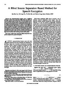
where A is an unknown matrix called the mixing matrix and x(t), s(t) are the two vectors representing the observed signals and source signals respectively. In this system we have no information about sources and how they mixed. Keywords— BSS, Discrete Wavelet Transform, Newton Method, To estimates sources, ICA present the “unmixing matrix” W, Nonlinear Autocorrelation, Speech processing where, W  A 1 (2) I. INTRODUCTION Now, the independent sources can be obtained: We are closured by sounds. Living in such a noisy places and sˆ(t )  Wx(t ) (3) obtain desired speech, makes it important to be able to The diagram in Figure 1 demonstrates both the mixing and separate and extract original speech signals from their mixtures in both man–machine and human–human unmixing process discussed in BSS. The independent sources communication. There is not enough information about are mixed with the matrix A. The goal is finding ‘'y’ that sources and channel characteristics, so any available approximates ‘s’ by estimating the unmixing matrix W. If the information must used to solve the problem. The problem of estimate of the unmixing matrix is precise, we receive a good estimating the sources from their mixtures can be expressed approximation of the sources. The described ICA model is as problems related to BSS. Using statistical properties of the simple model because it ignores all kind of noises and any original sources, ICA is one of the most used techniques for time delay in the recordings [2]. BSS. In BSS the word blind refers to the fact that we do not know how the signals were mixed or how they were generated. There are many algorithms for BSS using the statistical properties of source signals such as non-gaussianity, smoothness , linear autocorrelation ,temporal algorithms , nonstationarity ,sparsity , nonnegativity, and nonlinear autocorrelation. Zhenewi Shi also proposed a fast method for Fig1. Mixing and unmixing process involved in BSS solving the BSS problems using the non- Gaussianity and nonlinear temporal autocorrelation structure assumption. They applied Newton algorithm in time-domain as an iterative method for signal separation [11]. In compare with the well-known linear autocorrelation, nonlinear autocorrelation is a novel statistical property for BSS. In this paper, we have proposed a nonlinear BSS B. Whitening algorithm. It is based on nonlinear autocorrelation function. Run in wavelet domain accessed better separation accuracy and high speed convergence than Shi’s algorithm. ©IJEECS

(IJEECS) International Journal of Electrical, Electronics and Computer Systems. Vol: 13 Issue: 02, 2013 Another step for BSS is prewhitening the observation vector x. It can be expressed that whitening solves half of the ICA problem. It is very useful step and significantly reduces the computational complexity of ICA. Our another step to obtain better separation is prewhiten vector x, too. when signal whitened, its components are uncorrelated and have unit variance [27]. Let x w denote the whitened

vector,

then

we

have

following

equation:

E{x w x }  I T w

(4)

where E{x x } is the covariance matrix of x w . As you know ICA framework is insensitive to the variances of the independent components, so without loss of generality, the source vector, s, is white, i.e. E{ss T }  I Using the eigenvalue decomposition (EVD) of x, one can easily perform the whitening transformation. That is, we decompose the covariance matrix of x as follows: E{ xx T }  VDV T (5)

The Newton algorithm requires the inverse of Hessian matrix in 12 which is generally difficult to compute. Based on the BSS assumption the Hessian matrix becomes diagonal and can easily be invert.

 2 E{G( ~ y (t ))G( ~ y (t  ))}  I (where  E{g( ~ y (t ))G( ~ y (t  )) 2 w  G( ~ y (t ))g( ~ y (t  ))  g ( ~ y (t ))g ( ~ y (t  ))  g ( ~ y (t ))g ( ~ y (t  ))} (13) Where the function g is the derivative of G.

T w w

T

where V is the matrix of eigenvectors of E{xx } , and D is the diagonal matrix of eigenvalues, i.e. D  diag{1 , 2 ,..., n } . Now we have whitened signal as follow:

III. DISCRETE WAVELET TRANSFORM To overcome the problems of short time Fourier Transform (STFT) which are related to its frequency and time resolution properties wavelet transform was developed. In this transform unlike STFT that provides uniform time resolution for all frequencies, the DWT provides high time resolution and low frequency resolution for high frequencies and high frequency resolution for low frequencies [8]. The (DWT) is defined by the following equations:

W ( j, k )    x(k )Q j k



j 2

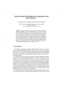
(14) where y(t) is a function with finite energy and fast decay (6) called mother wavelet. The DWT analysis accomplished It is uncorrelated and has unit variance. using a fast, pyramidal algorithm related to multi rate filter bank and presented as a constant Q filter bank with octave C. Objective Function spacing between the centres of the filters. If we decompose As it has been described above, in BSS problem the object is the signal into a coarse estimation, each sub-band contains estimating the separating matrix W. half the samples of the neighboring higher frequency bands T y( t )  w x ( t ) (7) with different resolution. Because of equalization between the number of resulting y (t   )  wT x(t   ) (8) wavelet coefficient and the number of input points in down Where ‘W’ is the unknown vector that must be acquired sampling, the Discrete Wavelet Transform (DWT) can be using ICA and  is some lag constant, usually equal to 1. expressed as a relatively recent and computationally efficient First of all, the measured signals x has been whitened using technique for extracting information and spectral properties matrix V, ~ x (t ) have unit of non-stationary signals like audio. x (t )  vx(t ) . So the components of ~ variance and uncorrelated. To obtaining the ‘W’ vector we Another step is using the process known as inverse discrete will use the nonlinear autocorrelation of estimated signals as waveform transform and reconstructing coefficient back into the original signal. Much like the DWT, the IDWT can be an object function and maximized it. ~ ~ explained by using filter bank theory, so the process is simply max w 1  ( w)  E{G ( y (t ))G ( y (t   ))} reversed [3]. Figure 2 shows DWT and IDWT process where:  E{G ( w T ~ x (t ))G ( w T ~ x (t   ))} (9) Where G is a differentiable nonlinear function, that measure X z  - Input signal the desired source’s nonlinear autocorrelation degree [11]. Xˆ  z  - Reconstructed signal H- Decomposition filter D. Learning Algorithm F- Decomposition filter To maximizing the objective function defined by 9 Newton X z  X 0 z  V z  ---------0 iteration described as follow: H0 F0 3 3 2 ~ ~  E{G ( y (t ))G ( y (t   ))} 1 V1 z  w  w( ) X 1 z  --------H1 F1  3 3 w2 ~ ~ E{G ( y (t ))G ( y (t   ))} V2 z  X 2 z  Xˆ z  ( ) (10) --------H2 F2  3 3 w (11) w  w/ w 1  2

x w  VD V T x

Where, E{G ( ~ y (t ))G ( ~ y (t   ))} w  E{g ( ~ y (t ))G ( ~ y (t   )) ~ x (t )G ( ~ y (t )) g ( ~ y (t   )) ~ x (t   )}

Fig2. DWT and IDWT process

(12)

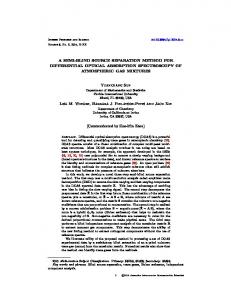
IV. SIMULATION REZULT The block diagram shows in figure 3 explains the overview of our nonlinear algorithm. The input signal is taken as mixed signal.

©IJEECS

(IJEECS) International Journal of Electrical, Electronics and Computer Systems. Vol: 13 Issue: 02, 2013 It is assumed that source signals are zero mean and unit variances, which shown as figure 4. These signals are mixed using a random mixing matrix and the mixing signals are obtained as an observation signals. The mixing signals are plotted in figure 5. The mixed signals are whitened to possess unit variance and then decomposed using DWT. The next step is to apply nonlinear autocorrelation algorithm based Newton method. Now the separated signals are reconstructed using IDWT. At last Signal to Noise Ratio (SNR) and Performance Index (PI) are measured. These parameters are defined as the following equations [11]:  var s t    SNR  10 log   var s t   sˆ t   (15)



amplitude

0 -10 0

amplitude

(16)

n  1n rPIi  cPIj  2  n  i1 j 1 

10

 n n  pij pij 1  n  n     1  1      n2  i1  j 1 maxk pik  j 1  i1 maxk pkj      

1

10

2 time

3

2 time

3

2 time

3

4

4

x 10

0 -10 0

amplitude

PI 

Fig5. Mixing Signals

1

20

4

4

x 10

0 -20 0

1

4

4

x 10

Fig6. Estimated Speech Signals 0.1 time domain wavelet domain

0.09 0.08 0.07 0.06 0.05 0.04 0.03 0.02 0.01

Fig3. Block diagram of proposed algorithm

0

In the PI parameter p ij is the i, j th element of P=W×V×A

amplitude amplitude amplitude

0

20

2 time

3

2 time

3

10

2 time

3

4

4

x 10

amplitude amplitude ude

SNR ( db ) 1

SNR ( db ) 2

SNR ( db ) 3

Time

21.45574

38.4581

22.1589

33.2001

54.4592

31.5840

domain

0 -10 0

1

4

4

x 10

0 1

10

2 time

3

V. CONCLUTION In this paper we use a nonlinear algorithm based on Newton algorithm to separate source signals and run our algorithm in wavelet domain. As described above, Discrete Wavelet Transform and running algorithms in wavelet domain increase efficiency of the algorithm. Mixing signals are observed signals. First, mixed speech signals were whitened to have unit variance and be uncorrelated; then, they were decomposed into different frequency domains by DWT and the sub bands of speech signals were separated using the proposed algorithm in each wavelet domain.

4 x 104

©IJEECS

0

10

30

4

10

-10 0

25

domain

x 10

Fig4. Speech Source Signals

-10 0

20

Method

Wavelet 1

15

4

0 -20 0

10

Table 1. SIR parameter of Estimated Speech Signals for both methods

10

1

5

Fig7. PI parameter for time and wavelet domain

matrix. The larger value PI is the poorer statistical performance of the BSS algorithm. In figure 7-8 the PI Parameter for both methods are plotted. Also, in table 1 SNR parameter for the estimated source signal are shown.

-10 0

0

1

2 time

3

4 x 104

(IJEECS) International Journal of Electrical, Electronics and Computer Systems. Vol: 13 Issue: 02, 2013 At last, source signals were reconstructed from single branches. To obtaining of accuracy of the proposed algorithm, the performance index and SIR parameter are calculated. It is shown that the proposed algorithm gets better results than the other methods. The sampling rate of signals is 16000 samples per second which selected from TIMIT database.

VI. REFRENCES [1]. M.S. Lewicki, T.J. Sejnowski, “Learning over complete representations”, Neural Computation Vol. 12, Issue 2, 2000, pp. 337–365. [2]. Ganesh R. Naik, Dinesh K Kumar, “An Overview of Independent Component Analysis and Its Applications”, Informatica 35 Vol. 63, Issue 81, 2011, pp. 63-81 [3]. A.Wims Magdalene Mary, Anto Prem Kumar, Anish Abraham Chacko, “blind source separation using wavelets”, IEEE International Conference on Computational Intelligence and Computing Research, 2010 [4]. Fabian J. Theis, Peter Gruber, Ingo R. Keck, Anke Meyer-Base, Elmar W. Lang, “spatiotemporal blind source separation using double-side approximate joint diagonalization” [5]. Z. Shi, H. Tang, Y. “Tang, Blind source separation of more sources than mixtures using sparse mixture models”, Pattern Recognition Letters Vol. 26, Issue 16, 2005, pp. 2491–2499. [6]. M. Zibulevsky, B.A. Pearlmutter, “Blind source separation by sparse decomposition in a signal dictionary”, Neural Computation Vol. 13 , 2001, pp. 863–882. [7]. E. Oja, M.D. Plumbley, “Blind separation of positive sources by globally convergent gradient search”, Neural Computation Vol. 16, Issue 9, 2004, pp. 1811–1825. [8]. M.D. Plumbley, E. Oja, A “non-negative PCA” algorithm for independent component analysis”, IEEE Transactions on Neural Networks Vol. 15, Issue 1, 2004, pp. 66–76. [9]. Z. Shi, C. Zhang, “Nonlinear innovation to blind source separation”, Neurocomputing Vol. 71, 2007, pp. 406–410. [10]. Z. Shi, Z. Jiang, F. Zhou, “A fixed-point algorithm for blind source separation with nonlinear autocorrelation”, Journal of Computational and Applied Mathematics Vol. 223, Issue 2, 2008, pp. 908-915 [11]. Zhenwei Shi, Changshui Zhang, “Fast nonlinear autocorrelation algorithm for source separation”, Pattern Recognition, 2008, doi: 10.1016/j.patcog.2008.12.025. [12]. Zhenwei Shi _, Zhiguo Jiang, Fugen Zhou, Jihao Yin, “Blind source separation with nonlinear autocorrelation and non- Gaussianity”, Journal of Computational and Applied Mathematics Vol. 229, Issue 1, 2009, pp. 240_247 [13]. Z.Y. Liu, K.C. Chiu, L. Xu, “One-bit-matching conjecture for independent component analysis”, Neural Computation Vol. 16, 2004, pp. 383–399 [14]. A.K. Barros, A .Cichocki, “Extraction of specific signals with temporal structure”, Neural Computation Vol. 13, Issue 9, 2001, pp.1995–2003. [15]. L. Tong, R.-W. Liu, V. Soon, Y.-F. Huang, “Indeterminacy and identifiability of blind identification”, IEEE Transactions on Circuits and Systems Vol. 38, Issue 5, 1991, pp. 499–509. [16]. A. Belouchrani, K.A. Meraim, J.-F. Cardoso, E.Moulines, “A blind source separation technique based on

second order statistics”, IEEE Transactions on Signal Processing Vol. 45, Issue 2, 1997, pp. 434–444. [17]. J.V. Stone, “Blind source separation using temporal predictability”, Neural Computation Vol. 13, 2001, pp. 1559– 1574. [18]. S.I. Amari, A. Cichocki, H.H. Yang, A new learning algorithm for blind source separation, Advances in Neural Information Processing Systems Vol. 8, 1996, pp. 757–763. [19]. A. Bell, T. Sejnowski, “An information-maximization approach to blind separation and blind deconvolution”, Neural Computation vol. 7, Issue 6, 1995, pp. 1129–1159. [20]. Ganesh R. Naik, Dinesh K Kumar, “An Overview of Independent Component Analysis and Its Applications”, Informatica 35 Vol. 63, Issue 81, 2011, pp. 63-81 [21]. A.Wims Magdalene Mary, Anto Prem Kumar, Anish Abraham Chacko, “blind source separation using wavelets”, IEEE International Conference on Computational Intelligence and Computing Research, 2010 [22]. Fabian J. Theis, Peter Gruber, Ingo R. Keck, Anke Meyer-Base, Elmar W. Lang, “spatiotemporal blind source separation using double-side approximate joint diagonalization” [23]. J.-F.Cardoso, B.H. Laheld, Equivariant “adaptive source separation”, IEEE Transactions on Signal Processing vol. 44, Issue 12, 1996, pp. 3017–3030. [24]. A.Cichocki, S.-I. Amari, “Adaptive Blind Signal and Image Processing: Learning Algorithms and Applications”, Wiley, NewYork

©IJEECS