A Parallel Software-Only Video Effects Processing System

A Parallel Software-Only Video Eects Processing System by Ketan Dasharath Mayer-Patel B.A. (University of California, Berkeley) 1992 M.S. (University of California, Berkeley) 1997 A dissertation submitted in partial satisfaction of the requirements for the degree of Doctor of Philosophy in Computer Science in the GRADUATE DIVISION of the UNIVERSITY of CALIFORNIA at BERKELEY Committee in charge: Professor Lawrence A. Rowe, Chair Professor Steven Ray McCanne Professor Ray Larson

Fall 1999

The dissertation of Ketan Dasharath Mayer-Patel is approved:

Chair

Date

Date

Date

University of California at Berkeley Fall 1999

A Parallel Software-Only Video Eects Processing System

Copyright 1999 by Ketan Dasharath Mayer-Patel

1

Abstract A Parallel Software-Only Video Eects Processing System by Ketan Dasharath Mayer-Patel Doctor of Philosophy in Computer Science University of California at Berkeley Professor Lawrence A. Rowe, Chair Video is playing an increasingly important role as an Internet media data type. Internet video use, however, typically means streaming live or on-demand material without manipulation. One important class of operations is video eects processing such as titling, compositing, and blending. Experience from the television, video, and lm industries shows that video eects are an important tool for communicating information and maintaining audience interest. In most applications, video is created in traditional studio settings, edited with special purpose hardware, and nally digitized and compressed for Internet streaming. We envision that streaming video on the Internet will become a rst-class data type that can be manipulated in real-time. As such, a network-based model centered around a compressed packet stream representation is needed instead of the traditional model centered around an uncompressed synchronous stream representation. In this new model, video sources will be compressed packet video streaming across a network from cameras connected to computers and video-on-demand archives. The destination of the processed video will include archival systems, content indexing systems, and viewers watching the video. In this way, video eects processing will be incorporated into a variety of applications including distance learning, collaborative virtual meetings, remote training, news and entertainment. This dissertation describes a software-only video eects processing system designed for the compressed packet video environment. We call this system the Parallel Software-only Video Eects Processing system (PSVP). A software-only solution using

2 commodity hardware provides the exibility required to handle compressed video sources. Variable frame rates, packet loss, and jitter which are attributes of Internet video can be handled gracefully with dynamic adaptation. A software solution provides exibility to adapt to new video formats and communication protocols and bene t from continuing improvements in processor and networking technology. The key to a software solution is exploiting parallelism. Currently, a single processor cannot produce a wide variety of real-time video eects which is why conventional systems and early research systems use custom-designed hardware. Even as processors become faster, the demand for more complicated eects, larger images, and higher quality will increase the video eects processing requirements. A scalable software solution is required to meet these growing application demands. The quality of video used on the Internet today is quite poor and is unlike CD quality audio which is near the limits of human perception. PSVP is a parallel solution that can incorporate additional computing resources to meet increased demands for higher quality. Fortunately, video processing algorithms contain a high degree of parallelism. Three types of parallelism can be exploited when implementing these algorithms: functional, temporal, and spatial. Functional parallelism can be exploited by decomposing the video eect task into smaller subtasks and mapping these subtasks onto dierent computational resources. Temporal parallelism can be exploited by demultiplexing the stream of video frames to dierent processors and multiplexing the processed output. For example, one processor may deal with all odd numbered frames while another deals with all even numbered frames. Spatial parallelism can be exploited by assigning regions of the video stream to dierent processors. For example, one processor may process the left half of all video frames while another deals with the right half. Taking advantage of these types of parallelism requires the solution of dierent problems. This dissertation describes our solution to some of these problems. Speci cally:

 A framework was developed to explore and implement parallel video eects using a network of workstations distributed computing system.

 Mechanisms were developed to exploit temporal and spatial parallelism.  A distributed control protocol was developed that provides per-message, receiverdriven reliability semantics.

3 Another problem encountered during this research is that video compression formats were designed for storage and transmission and not for manipulation. Transport protocols for packet video often assume that a video source originates from a single point in the network. These assumptions con ict with how a distributed software system, such as PSVP, might produce the video stream. The design choices made in building PSVP were heavily in uenced and sometimes constrained by the earlier design choices made by those who developed these standards and protocols. The dissertation describes these in uences and constraints. The overall lesson learned from developing PSVP is that video formats and protocols developed with transmission and storage as the primary applications create arti cial constraints for applications that manipulate packet video data.

Professor Lawrence A. Rowe Dissertation Committee Chair

iii

To Christine, whose love and support made all of this possible.

iv

Contents List of Figures List of Tables 1 Introduction 2 Background

2.1 Parallel Processing . . . . . . . . . . . . . 2.2 Multicast Protocols . . . . . . . . . . . . . 2.2.1 IP-Multicast . . . . . . . . . . . . 2.2.2 Real-Time Transport Protocol . . 2.2.3 Reliable Multicast Protocols . . . . 2.3 Video Compression and Transmission . . 2.3.1 Color Representation . . . . . . . . 2.3.2 Discrete Cosine Transform . . . . . 2.3.3 Intercoding . . . . . . . . . . . . . 2.3.4 Entropy Coding . . . . . . . . . . 2.4 Video Processing Hardware . . . . . . . . 2.5 Video Processing Software . . . . . . . . . 2.5.1 Language and Development Tools 2.5.2 Parallel Video Processing Software 2.6 Summary . . . . . . . . . . . . . . . . . .

3 System Design and Architecture 3.1 3.2 3.3 3.4 3.5 3.6 3.7 3.8

System Components . . Resource Model . . . . . Data Model . . . . . . . Software Architecture . Eect-Plan Abstraction Control Issues . . . . . . Evaluation Metrics . . . Summary . . . . . . . .

. . . . . . . .

. . . . . . . .

. . . . . . . .

. . . . . . . .

. . . . . . . .

. . . . . . . .

. . . . . . . .

. . . . . . . .

. . . . . . . .

. . . . . . . .

. . . . . . . . . . . . . . .

. . . . . . . . . . . . . . .

. . . . . . . . . . . . . . .

. . . . . . . . . . . . . . .

. . . . . . . . . . . . . . .

. . . . . . . . . . . . . . .

. . . . . . . . . . . . . . .

. . . . . . . . . . . . . . .

. . . . . . . . . . . . . . .

. . . . . . . . . . . . . . .

. . . . . . . . . . . . . . .

. . . . . . . . . . . . . . .

. . . . . . . . . . . . . . .

. . . . . . . . . . . . . . .

. . . . . . . . . . . . . . .

. . . . . . . . . . . . . . .

. . . . . . . . . . . . . . .

. . . . . . . . . . . . . . .

. . . . . . . . . . . . . . .

. . . . . . . .

. . . . . . . .

. . . . . . . .

. . . . . . . .

. . . . . . . .

. . . . . . . .

. . . . . . . .

. . . . . . . .

. . . . . . . .

. . . . . . . .

. . . . . . . .

. . . . . . . .

. . . . . . . .

. . . . . . . .

. . . . . . . .

. . . . . . . .

. . . . . . . .

. . . . . . . .

. . . . . . . .

vi ix 1 10 10 11 12 12 13 13 13 14 14 17 17 19 20 21 22

23

24 29 33 35 42 53 54 55

v

4 Implementation

4.1 FX Processor . . . . . . . . . . . . . . . . . . . . 4.1.1 MASH . . . . . . . . . . . . . . . . . . . . 4.1.2 Dali . . . . . . . . . . . . . . . . . . . . . 4.2 Execution Example . . . . . . . . . . . . . . . . . 4.3 FX Mapper . . . . . . . . . . . . . . . . . . . . . 4.3.1 Operators, Parameters, and Video Buers 4.3.2 Code Generation . . . . . . . . . . . . . . 4.4 Summary . . . . . . . . . . . . . . . . . . . . . .

5 Temporal Parallelism 5.1 5.2 5.3 5.4 5.5

Temporal Parallelism Mechanics . Selector Function . . . . . . . . . . Interleaver Function . . . . . . . . Temporal Mechanism Performance Summary . . . . . . . . . . . . . .

. . . . .

. . . . . . . .

. . . . . . . .

. . . . . . . .

. . . . . . . .

. . . . . . . .

. . . . . . . .

. . . . . . . .

. . . . . . . .

. . . . . . . .

. . . . . . . .

. . . . . . . .

. . . . . . . .

. . . . . . . .

. . . . . . . .

. . . . . . . .

57

57 58 60 62 69 70 72 76

77

. . . . .

. . . . .

. . . . .

. . . . .

. . . . .

. . . . .

. . . . .

. . . . .

. . . . .

. . . . .

. . . . .

. . . . .

. . . . .

. . . . .

. . . . .

. . . . .

. . . . .

. . . . .

. . . . .

. . . . .

. . . . .

. 78 . 81 . 89 . 97 . 102

6.1 Input Distribution . . . . . . . . . . . 6.2 Output Reconstruction . . . . . . . . . 6.3 Format Details . . . . . . . . . . . . . 6.3.1 Format Measurements . . . . . 6.3.2 SC Format Size . . . . . . . . . 6.3.3 Encoder/Decoder Performance 6.4 Performance . . . . . . . . . . . . . . . 6.5 Summary . . . . . . . . . . . . . . . .

. . . . . . . .

. . . . . . . .

. . . . . . . .

. . . . . . . .

. . . . . . . .

. . . . . . . .

. . . . . . . .

. . . . . . . .

. . . . . . . .

. . . . . . . .

. . . . . . . .

. . . . . . . .

. . . . . . . .

. . . . . . . .

. . . . . . . .

. . . . . . . .

. . . . . . . .

. . . . . . . .

. . . . . . . .

. . . . . . . .

. 106 . 112 . 114 . 119 . 119 . 121 . 123 . 127

FX Processor Organization . . . . . . . Type and Structure of Control Messages Control Requirements . . . . . . . . . . SRM and SNAP . . . . . . . . . . . . . PSVP Control . . . . . . . . . . . . . . . Control Mapping Feature . . . . . . . . Summary . . . . . . . . . . . . . . . . .

. . . . . . .

. . . . . . .

. . . . . . .

. . . . . . .

. . . . . . .

. . . . . . .

. . . . . . .

. . . . . . .

. . . . . . .

. . . . . . .

. . . . . . .

. . . . . . .

. . . . . . .

. . . . . . .

. . . . . . .

. . . . . . .

. . . . . . .

. . . . . . .

. . . . . . .

. 128 . 134 . 138 . 140 . 141 . 143 . 151

. . . .

. . . .

. . . .

. . . .

. . . .

. . . .

. . . .

. . . .

. . . .

. . . .

. . . .

. . . .

. . . .

. . . .

. . . .

. . . .

. . . .

. . . .

. . . .

. 152 . 155 . 156 . 157

6 Spatial Parallelism

7 Control Protocol 7.1 7.2 7.3 7.4 7.5 7.6 7.7

8 Conclusions and Future Work 8.1 8.2 8.3 8.4

Review of Motivations and Design Research Contributions . . . . . . Future Research Directions . . . . Summary . . . . . . . . . . . . . .

Bibliography

. . . .

. . . .

. . . .

103

128

152

159

vi

List of Figures 1.1 1.2 1.3 1.4

Sample Video Eects . . . . . . . . . . . . . . . A Video Production Switcher . . . . . . . . . . Typical Broadcast Production Model . . . . . . Network-based Packet Video Production Model

. . . .

. . . .

. . . .

. . . .

. . . .

. . . .

. . . .

. . . .

. . . .

. . . .

. . . .

. . . .

. . . .

. . . .

. . . .

. . . .

2 3 4 5

2.1 DCT Encoding Process . . . . . . . . . . . . . . . . . . . . . . . . . . . . . 15 2.2 MPEG Interframe Dependencies . . . . . . . . . . . . . . . . . . . . . . . . 16 3.1 3.2 3.3 3.4 3.5 3.6 3.7 3.8 3.9 3.10 3.11 3.12 3.13 3.14 3.15 3.16 3.17 3.18 3.19

PSVP System Architecture . . . . . . . . . . . . . . . . . . . . . . . . Distance Learning Scenario Components . . . . . . . . . . . . . . . . . VVPS User Interface . . . . . . . . . . . . . . . . . . . . . . . . . . . . RTP Packet Format . . . . . . . . . . . . . . . . . . . . . . . . . . . . PSVP Software Architecture . . . . . . . . . . . . . . . . . . . . . . . Cross-Dissolve Eect . . . . . . . . . . . . . . . . . . . . . . . . . . . . Simple Cross-Dissolve Graph Representation . . . . . . . . . . . . . . Cross-Dissolve Eect Using Functional Parallelism . . . . . . . . . . . Cross-Dissolve Eect Using Temporal Parallelism . . . . . . . . . . . . Cross-Dissolve Eect Using Spatial Parallelism . . . . . . . . . . . . . Legend for Symbols in Eect-Plans . . . . . . . . . . . . . . . . . . . . Cross-Dissolve Eect-Plan Representation . . . . . . . . . . . . . . . . Cross-Dissolve Eect-Plan Representation with Temporal Parallelism . Cross-Dissolve Eect-Plan Representation with Spatial Parallelism . . Cross-Dissolve Eect-Plan Representation with Functional Parallelism Hierarchical Cross-Dissolve Plan, Level 1 . . . . . . . . . . . . . . . . . Hierarchical Cross-Dissolve Plan, Level 2 . . . . . . . . . . . . . . . . . Hierarchical Cross-Dissolve Plan, Level 3 . . . . . . . . . . . . . . . . . Eect-Plan Hierarchy for Cross-Dissolve Example . . . . . . . . . . . .

. . . . . . . . . . . . . . . . . . .

. . . . . . . . . . . . . . . . . . .

. . . . . . . . . . . . . . . . . . .

24 26 27 35 36 37 38 39 40 41 42 44 45 47 48 50 51 52 53

4.1 4.2 4.3 4.4 4.5 4.6

FX Processor Object Block Diagram . . . . . . . . . . . . . . . . . . . . . . Picture-in-Picture Subprogram Init Method . . . . . . . . . . . . . . . . . . Picture-in-Picture Subprogram Trigger Method, Part 1 . . . . . . . . . . . . Picture-in-Picture Subprogram Trigger Method, Part 2 . . . . . . . . . . . . Initialization Code Fragment For An Integer Parameter . . . . . . . . . . . Execution Code Fragment For The Uncompressed Scalar Multiply Operator

59 65 66 67 73 75

vii 5.1 5.2 5.3 5.4 5.5 5.6 5.7 5.8 5.9 5.10 5.11 5.12 5.13 5.14 5.15 5.16 5.17 5.18

Idealized Model for Temporal Parallelism . . . . . . . . . . . . . . . . . . . 78 Idealized Model for Temporal Parallelism with Varied Processing Times . . 80 An RTP Header . . . . . . . . . . . . . . . . . . . . . . . . . . . . . . . . . 82 Illustration of Non-Uniform Packet Loss Among Peer Processors . . . . . . 83 Full Cross-Dissolve Plan Representation with Temporal Parallelism . . . . . 88 Interleaver Buering Latency vs. , = 1:0 . . . . . . . . . . . . . . . . . . 93 Interleaver Frame Drop Percentage vs. , = 1:0 . . . . . . . . . . . . . . . 94 Interleaver Buering Latency and Frame Drop Percentage vs. , = 1:0, Sequence SD = 120 ms . . . . . . . . . . . . . . . . . . . . . . . . . . . . . . 94 Interleaver Buering Latency vs. , Varying , Sequence SD = 120 ms . . . 95 Interleaver Buering Frame Drop Percentage vs. , Varying , Sequence SD = 120 ms . . . . . . . . . . . . . . . . . . . . . . . . . . . . . . . . . . . 95 Achieved Frame Rate for 590 kb/s MJPEG Video with Temporal Parallelism 97 Achieved Frame Rate for 900 kb/s MJPEG Video with Temporal Parallelism 98 Achieved Frame Rate for 1.2 Mb/s MJPEG Video with Temporal Parallelism 98 Achieved Frame Rate for 1.5 Mb/s MJPEG Video with Temporal Parallelism 99 Achieved Frame Rate for 280 kb/s H.261 Video with Temporal Parallelism 100 Achieved Frame Rate for 560 kb/s H.261 Video with Temporal Parallelism 100 Achieved Frame Rate for 750 kb/s H.261 Video with Temporal Parallelism 101 Achieved Frame Rate for 900 kb/s H.261 Video with Temporal Parallelism 101

6.1 Idealized Models for Spatial Parallelism For 1, 2, and 4 Processes . . . . . . 104 6.2 Partial Output Regions and Corresponding Input Regions For A Rotation Eect . . . . . . . . . . . . . . . . . . . . . . . . . . . . . . . . . . . . . . . 107 6.3 Partial Output Regions and Corresponding Input Regions For A PictureIn-Picture Eect . . . . . . . . . . . . . . . . . . . . . . . . . . . . . . . . . 108 6.4 Example Eect-Plan Using Spatial Parallelism . . . . . . . . . . . . . . . . 111 6.5 SC Packet Format . . . . . . . . . . . . . . . . . . . . . . . . . . . . . . . . 115 6.6 RTP Header . . . . . . . . . . . . . . . . . . . . . . . . . . . . . . . . . . . . 115 6.7 SC Header . . . . . . . . . . . . . . . . . . . . . . . . . . . . . . . . . . . . . 116 6.8 Block Addressing . . . . . . . . . . . . . . . . . . . . . . . . . . . . . . . . . 117 6.9 Block Encoding . . . . . . . . . . . . . . . . . . . . . . . . . . . . . . . . . . 118 6.10 Ratio of SC frame size to M-JPEG frame size vs. Bytes Per M-JPEG Block.120 6.11 SC Encoding Time Per Block in Microseconds vs. Quality Factor . . . . . . 121 6.12 SC Encoding Time In Milliseconds vs. Quality Factor For Various Region Sizes . . . . . . . . . . . . . . . . . . . . . . . . . . . . . . . . . . . . . . . . 122 6.13 Time Required To Transcode From SC to M-JPEG . . . . . . . . . . . . . . 122 6.14 Performance of Spatial Mechanism . . . . . . . . . . . . . . . . . . . . . . . 124 6.15 Performance of Hybrid Temporal/Spatial Mechanism . . . . . . . . . . . . . 126 7.1 7.2 7.3 7.4 7.5

Cross-Dissolve Eect-Graph . . . . . . . . . . . . . . . . . . . Cross-Dissolve Eect-Plan . . . . . . . . . . . . . . . . . . . . Legend for Symbols in Eect-Plans . . . . . . . . . . . . . . . Cross Dissolve Execution Plan Adding Temporal Parallelism Cross-Dissolve Execution Plan Adding Spatial Parallelism . .

. . . . .

. . . . .

. . . . .

. . . . .

. . . . .

. . . . .

. . . . .

. 129 . 130 . 131 . 132 . 133

viii 7.6 7.7 7.8 7.9 7.10 7.11 7.12

Cross-Dissolve Execution Plan Adding Function Parallelism . . . . . . . . . 135 Cross-Dissolve Execution Plan Hierarchy . . . . . . . . . . . . . . . . . . . . 136 Overview of Control Information Flow . . . . . . . . . . . . . . . . . . . . . 136 Control Namespace for Cross-Dissolve . . . . . . . . . . . . . . . . . . . . . 142 Control Relationships With Temporal Parallelism . . . . . . . . . . . . . . . 144 Control Relationships With Temporal Parallelism After Control Mapping . 148 Time required to distribute control messages to a shallow hierarchy of varying width. . . . . . . . . . . . . . . . . . . . . . . . . . . . . . . . . . . . . . 150 7.13 Time required to distribute control messages to a binary hierarchy of varying depth. . . . . . . . . . . . . . . . . . . . . . . . . . . . . . . . . . . . . . . . 150 8.1 PSVP System Architecture . . . . . . . . . . . . . . . . . . . . . . . . . . . 153 8.2 PSVP Software Architecture . . . . . . . . . . . . . . . . . . . . . . . . . . 154

ix

List of Tables 4.1 4.2 4.3 4.4 4.5

Dali Buer Types . . . . . . . . . Example Dali Commands . . . . VidRep Members and Methods . Examples of Operator Types . . Parameter Types and Attributes

. . . . .

. . . . .

. . . . .

. . . . .

. . . . .

. . . . .

. . . . .

. . . . .

. . . . .

. . . . .

. . . . .

. . . . .

. . . . .

. . . . .

. . . . .

. . . . .

. . . . .

. . . . .

. . . . .

. . . . .

. . . . .

. . . . .

. . . . .

. . . . .

60 61 63 70 71

6.1 Uncompressed Video Sizes and Bitrates . . . . . . . . . . . . . . . . . . . . 113 7.1 Common Attributes For Inputs, Outputs, and Parameters. . . . . . . . . . . 137 7.2 Description of Trigger Types . . . . . . . . . . . . . . . . . . . . . . . . . . 138 7.3 Description of map commands currently implemented. . . . . . . . . . . . . 147

x

Acknowledgements Acknowledging everyone who helped, guided, and supported me through the process of producing this dissertation would be a document twice as long as the dissertation itself. To all of those that I could not mention by name, accept my apologies and rest assured I appreciate everything you all have done for me. I would like to speci cally thank a number of people. I thank Larry Rowe for his guidance and friendship. Years ago he oered me a chance to demonstrate what I could accomplish and an environment in which I could grow. Brian Smith took time to mentor me as a young researcher and continues to provide me with excellent advice. Steve McCanne taught me how to evaluate the world of research with a critical eye and I appreciate his friendship and candor. Ray Larson was an excellent dissertation committee member and I have enjoyed interacting with him both in and out of the classroom. To all of the members of Alexis and Birk Club (and you know who you are), thanks for helping me relax and enjoy the graduate school experience to its fullest. To Mom, Dad, Mom Mayer, and Dad Mayer, thank you for your support, love, and encouragement. To Bhai, your advice to come to California for college started it all. Thank you for everything you've done for me. To Christine, you are my world and I love you very much. Go Bears! Beat Stanford!

1

Chapter 1

Introduction Video is playing an increasingly important role as an Internet multimedia data type. The growth of the World Wide Web (WWW) has given rise to a market for network technologies that provide high-speed access to the home. These technologies include ISDN, xDSL, and cable modems. As more homes have high-speed access, the importance of video increases. Even in the absence of high-speed access, low bit-rate encodings of video are prevalent. The emergence of video as a data type has also been caused by the creation of standardized compression schemes and transport protocols in combination with advances in processor technology that make software-only video decoding possible. Today, the uses of video as a data type on the Internet are many and varied. These uses include:

 Information. Television news stories from CNN, MSNBC, PBS, and other major television networks are available on a video-on-demand basis. Some television stations are beginning live broadcasts of news programs as well [15].

 Entertainment. Movies, non-news television shows, and other forms of entertainment

are available both on a subscriber basis and on an advertising supported basis. Broadcast.com, for example, provides free access to hundreds of movies, pre-recorded television shows, and live sporting events.

 Promotion. Advertisements for products are freely available for viewing through the

companies that produce them. Most movie production companies provide access to previews and trailers for newly released and upcoming movies.

2

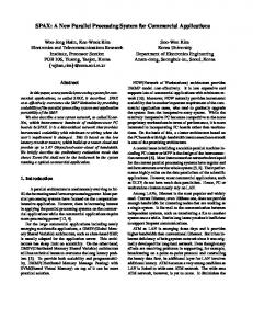
Titling

Transition Effect

Compositing

Figure 1.1: Sample Video Eects

 Distance Learning. Several major universities are experimenting with distance learn-

ing by providing lecture material over the Internet. For example, the Berkeley Multimedia Research Center at the University of California produces broadcasts of several dierent classes. These classes can be viewed live and can also be accessed through an archive system for on-demand replay [10, 59].

 Video Conferencing. The Multicast Backbone (MBone) conferencing tools vic and

vat as well as NetMeeting from Microsoft and ProShare from Intel are examples of Internet packet video conferencing tools.

Use of video on the Internet, however, has not yet included manipulation of video data. In most of the above application areas, video is created in traditional studio settings, edited with special purpose hardware, and nally digitized and compressed for Internet streaming purposes. Typically, the video data was not originally produced for Internet streaming purposes. For example, most on-line video content available from the major television networks and from services like Broadcast.com are subsampled and digitized versions of video originally transmitted for television. Video conferencing and distance learning are notable exceptions. In these cases, raw video (i.e., unedited) is transmitted directly from a camera. One important subclass of video manipulation is video eects processing. Experience from the television, video, and lm industries shows that special eects are an important tool for communicating and maintaining audience interest [43]. Almost all edited video contains some sort of video eect. Video eects are ubiquitous because they are eective. Titling, for example, is used to identify speakers and topics in a video presentation. Compositing eects that combine two or more video images into one image

3

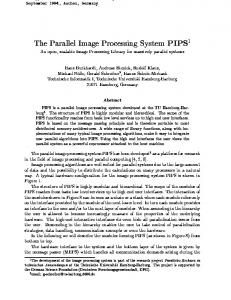
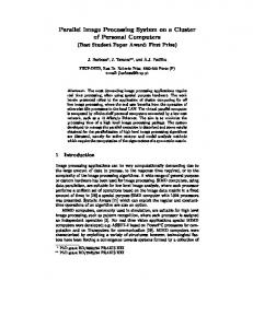
Figure 1.2: A Video Production Switcher are used to present simultaneous views of people or events at dierent locations. Blends, fades, and wipes are transition eects that ease viewers from one video source to another. Figure 1.1 shows examples of some of these eects. Traditionally, video eects are created using a video production switcher (VPS). A VPS is a specialized hardware device that manipulates analog or digital video signals to create video eects. It is usually operated by a technician or director at a VPS control console. Figure 1.2 shows a Composium VPS produced by DF/X. Figure 1.3 depicts a typical production model for creating a live video broadcast with eects and the role of a VPS in that process. Live video sources are produced by studio cameras, eld cameras, or remote locations transmitted to the studio via satellite. Stock footage, commercials, and other pre-recorded and edited material are accessed from archival systems (e.g., video tape recorders). In this setting, video data travels between components on specially designed analog or digital networks that are typically not packet based. A director, possibly working with a team of production technicians and cameramen, operates the VPS and other special-purpose hardware to create video eects and produce the broadcast. The resulting video data may be compressed and transmitted on an internet or intranet in a packet-based video format. The role of packet-based video formats in this production model is strictly as a transport for a nished product. Manipulation of the video after being encoded in a packet video format is rare. We envision that packet video data will become a rst-class multimedia data type that can be manipulated in real-time. As such, a network-based packet video manipulation model is needed instead of a traditional broadcast or o-line

4

Television broadcast.

Remote video signals via sattelite. Archived, pre-recorded video material.

VTR

VTR

Video Production Switcher

Camera source. Analog or digital video distribution network.

Capture and Compression

Figure 1.3: Typical Broadcast Production Model

Streaming packet video.

5 Effects Processor

Effects Processor

Effects Server Processed Video Output

Local Network Live Internet Video Source

Application Live Internet Video Source

Video Archive Server Video Control

Figure 1.4: Network-based Packet Video Production Model editing model centered around a special-purpose hardware VPS. In this new manipulation model, video sources will be compressed packet video streaming across a network from cameras connected to computers and video-on-demand archives. Figure 1.4 shows the network-based packet video manipulation model that we envision. Sources are compressed packet video streams generated either in the local environment or from across the Internet. Pre-recorded and edited material is accessed from video-on-demand archives. Software processes provide resource management and video processing capabilities. Using this environment, we enable a number of new and interesting applications using streaming compressed packet video. Distance learning environments can be enhanced with video eects to provide improved production quality. Multiple streams can be composited into new streams. For example, a stream showing a professor can be inset using a picture-in-picture eect within a stream showing the contents of a whiteboard or other instructional material. Another application might manipulate and process video streams from a set of security cameras to recognize interesting \events" (i.e., excessive motion, sudden change in lighting, etc.) and bring them to the attention of a security guard. A third application might be internationalization of video-on-demand

6 service by automatically inserting subtitles in a number of dierent languages depending on user preference. Instead of storing multiple copies of the video stream, each with subtitles already produced, the subtitles and information on when they appear can be stored compactly and separately from the video itself. When the user accesses the video, subtitles can be inserted into the stream as needed. One way to create a compressed packet video production system is to simply convert the compressed streams into a traditional video signal, use a VPS to manipulate the video, and recompress the resulting output. A conventional VPS, however, is not well matched for the packet video environment. An analog VPS requires signals with very tight timing constraints which are not present with compressed packet video. A digital VPS requires uncompressed signals and uses communication protocols not suitable for the Internet. Moreover, hardware VPS solutions can be very expensive. A VPS can cost anywhere from $1000 for a low-end model with very limited capabilities to $250,000 for a full-featured digital VPS like the Composium pictured in Figure 1.2. Compressed packet video is characterized by variable frame rates, bit rates, and jitter. Traditional hardware, whether analog or digital, depends on constant frame rates, constant bit rates, and tightly synchronized signaling. The goal of the work reported in this dissertation is to develop a software-only video eects processing system designed for the compressed packet video environment. We call this system the Parallel Software-only Video Eects Processing system (PSVP). A software-only solution using commodity hardware provides the exibility required to handle compressed video sources. Variable frame rates, packet loss, and jitter can be handled gracefully with dynamic adaptation. A software system can be written to handle compressed video formats already in use and extended for new formats as they are developed. And, standard multicast communication protocols (e.g., RTP [49]) can be used. Using general-purpose processors allows the system to bene t from continuous improvements in processor and networking technology. The key to a software solution is exploiting parallelism. Currently, a single processor cannot produce a variety of real-time video eects which is why conventional VPS systems and early research systems (e.g., Cheops [8]) use custom-designed hardware. Even as processors become faster, the demand for more complicated eects, larger images (e.g., HDTV), and higher quality will raise the bar for performance expected of a commodity hardware solution. The complexity of video eects processing is arbitrary because the

7 number, size, data rate, and quality of video streams is variable. Unlike CD quality audio, which is near the limits of human perception, the quality of video used on the Internet is quite poor. Improvements in processor and networking technology will be met with greater application demands. Fortunately, video processing contains a high degree of parallelism that can be exploited to solve this problem. Three types of parallelism can be used for video eects processing: functional, temporal, and spatial. Functional parallelism decomposes a video eect task into smaller subtasks and maps these subtasks onto the available computational resources. Temporal parallelism can be exploited by demultiplexing the stream of video frames to dierent processors and multiplexing the processed output. For example, one processor may deal with all odd numbered frames while another deals with all even numbered frames. Spatial parallelism can be exploited by assigning regions of the video frame image to dierent processors. For example, one processor may process the left half of all video frames while another deals with the right half. Taking advantage of these types of parallelism requires the solution of dierent problems. Exploiting functional parallelism requires the application of compilation techniques to produce an ecient decomposition of the processing task into smaller components. Temporal and spatial parallelism require mechanisms for distributing input video streams to the appropriate processor and recombining the resulting output stream. Another problem is caused by the fact that video compression formats were designed for storage and transmission and not for manipulation. Transport protocols for packet video often assume that a video source originates from a single point in the network. This assumption con icts with how a distributed software system might produce the video data stream. The design choices we made in building our system were heavily in uenced and sometimes constrained by earlier design choices made by groups that developed these standards and protocols. The major contributions of our work are:

 A framework was developed for exploring and implementing parallel video eects us-

ing a network of workstations. We integrated work done in multimedia toolkits, network-of-workstation parallel computing environments, and video manipulation languages into a system (i.e., PSVP) capable of expressing and executing complex video transformations. We

8 believe this system will serve as a basis for future research into how video can be manipulated and used as a rst class data type.

 A framework was developed for expressing video eect tasks as a directed acyclic

graph of operators. We developed a notation for expressing video eects as directed graphs of operators. These operators can be composed in dierent ways to create new eects. Given this graph notation, we have implemented a \compiler" that can generate an implementation of the eect that executes on our system. Although our compilation of an eect implementation is currently done in a straightforward and simple manner, the notation was designed to allow future research that can bring to bear optimization strategies that incorporate cost models for automatically and dynamically parallelizing video eect implementations.

 Mechanisms were developed for exploiting temporal parallelism with support for media

speci c temporal dependencies. We show how the design of these temporal parallelism mechanisms are in uenced and constrained by the design of media transport protocols and compression formats that did not foresee the need to pull apart, manipulate, and create video streams. In particular, we developed an adaptive buer management algorithm that allows a trade-o between buer latency and frame rate to be eectively managed.

 Mechanisms were developed for exploiting spatial parallelism.

As with the temporal mechanisms, we show how the design of spatial parallelism mechanisms are in uenced and constrained by current standards. We motivate and describe our development of a new compressed packet video format designed to allow several streams to describe spatially dierent areas of the same video stream. This new format was designed speci cally to facilitate integrating multiple partial streams (e.g., a stream describing the left half of a video frame and a stream describing the right half of a video stream) into one coherent stream. In particular, we show how techniques found in nearly every packet video standard complicate this type of manipulation and must be avoided.

 A distributed control protocol was constructed based on IP-Multicast using scalable reliable multicast technologies.

9 To support dynamic recon guration of video eect implementations, we deliberately chose a network technology that provides an abstraction between the communication channel and the location of participants (i.e., IP-Multicast). Delivering control messages with varying degrees of reliability in such an environment is problematic. We developed a control protocol on top of scalable reliable multicast technologies that provides a lightweight, highly exible solution. The remainder of this dissertation is organized as follows. Chapter 2 reviews related background work in a number of dierent areas including parallel processing, multicast protocols, video compression, video processing, and distributed multimedia toolkits. Chapter 3 describes the overall design of the PSVP system and each of its components. In Chapter 4, we describe speci c implementation details about some of these components. These details are necessary to understand how the design of the system was in uenced by the environment in which it was implemented. Chapter 5 describes the design and implementation of mechanisms used to exploit temporal parallelism, and Chapter 6 describes the design and implementation of mechanisms used to exploit spatial parallelism. Chapter 7 addresses the problem of distributing control messages using multicast technologies. Finally, Chapter 8 summarizes the dissertation and discusses a variety of interesting research areas and problems that remain to be studied using our system.

10

Chapter 2

Background The PSVP system incorporates ideas from numerous technologies including: parallel processing, multicast protocols, video compression and processing, and distributed multimedia toolkits. In this chapter, we review relevant work in each of these areas to provide a background for the rest of the dissertation.

2.1 Parallel Processing Parallel processing occurs when a collection of processing elements cooperatively operate on parts of a problem at the same time. In our case, the problem is computing video eects in real-time. Researchers have explored how parallel processing elements can be organized and programmed for more than thirty years. Recently, dierent parallel processing architectures have converged. This section introduces a taxonomy useful for describing parallel processing architectures, discusses the recent convergence of dierent architectures, and describes the Network-of-Workstations (NOW) architecture used by the PSVP system. Flynn developed a taxonomy for categorizing dierent parallel architectures in 1972 [25]. In his taxonomy, parallel architectures are distinguished by the number of dierent instructions performed and the number of data elements manipulated. A traditional processor that sequentially performs a single instruction on a single data element is classi ed as SISD (Single Instruction, Single Data). Parallel architectures are generally classi ed as either SIMD (Single Instruction, Multiple Data) or MIMD (Multiple Instruction, Multiple Data) architectures. Shared memory processors and message-passing

11 machines are two examples of MIMD parallel architectures. Data parallel machines and vector processors are categorized as SIMD architectures. Parallel machine architectures are converging to a generic MIMD architecture. The generic architecture is comprised of a collection of processors coupled with local memory and interconnected by a high-speed, low-latency communications network. Culler and Singh trace the history of this convergence and highlight the technological and economic pressures that caused it [17]. In the PSVP system, the \cooperating processing elements" are independent software components which communicate by transmitting streams of video data and control signals to each other. In this respect, the PSVP system is well suited for a generic MIMD architecture. Culler proposes that technological advances in network and processor technology allow high-performance parallel computers to be built from a collection of desktop machines [16]. Because the volume of desktop computers sold worldwide is large, the costs for development and innovation for desktop computers is smaller on a per unit basis than for tightly integrated massively parallel processors (MPP). Given smaller per unit innovation costs, the rate of improvement is faster for desktop machines. Constructing parallel computers from desktop machines capitalizes on this rate of innovation. The fruition of this work was the Berkeley Network-Of-Workstations (NOW) system [16]. The Berkeley NOW is a collection of 128 Sun UltraSPARC-1 workstations connected by a switched 10Mb/s Ethernet and a 160 MB/s Myrinet. The Ethernet network provides general connectivity among the workstations and to the rest of the Internet, while the Myrinet provides a highspeed, low-latency experimental network. Processing resources are managed on the NOW through a layer of software called the Global Layer UNIX (GLUnix) [26]. The PSVP system was built using GLUnix on the Berkeley NOW.

2.2 Multicast Protocols The software components of the PSVP system transmit video streams and control signals to each other as they cooperate to compute video eects. Because the same video and control data is often required by two or more components, the system uses communication protocols based on IP-Multicast. In this section, we review IP-Multicast and the IP-Multicast based protocols used by PSVP.

12

2.2.1 IP-Multicast The Internet Protocol (IP) is the basis for delivering packets of data on the Internet. The IP service model provides no guarantee of delivery. In addition, packets may arrive out of order. Packets are routed from source to destination based on the 32-bit destination IP address speci ed in the packet header. All possible sources and destinations have a unique IP address. This simple model is the basis for other protocols which provide additional services. The Transmission Control Protocol (TCP), for example, provides a reliable, congestion-controlled, byte-stream communication protocol that is implemented using IP. The User Datagram Protocol (UDP) provides a connectionless, datagram delivery protocol with error checking that is also implemented using IP. The IP-Multicast model, rst proposed by Deering [18], extends the traditional IP service model to deliver packets to multiple destinations eciently. Similar to IP, IP-Multicast makes no delivery guarantee. Any subset of the group may receive any given data packet. Order is also not guaranteed. The IP-Multicast delivery mechanism is ecient because packets are replicated in the network as necessary to reach members of the group. Thus, the sender of a multicast packet transmits only one copy of the data and does not need to know how large the group is nor where the group members are located. The network is responsible for delivering packets to group members no matter where they are located. Groups are identi ed by an IP-Multicast address. These addresses represent a communication session which users can join or leave at any time. IP-Multicast addresses are dynamically allocated from a reserved range of IP addresses.

2.2.2 Real-Time Transport Protocol The Real-Time Transport Protocol (RTP) is an Internet Engineering Task Force (IETF) standard for streaming transmission of media data [49]. Although independent of the underlying network technology, PSVP uses RTP with UDP and IP-Multicast to send and receive video data. Each RTP packet is comprised of an RTP header followed by a format speci c payload. The RTP header provides basic information about the data including the format of the payload, a media speci c timestamp for synchronization, a packet sequence number for detecting lost or duplicate packets, and a source identi er to distinguish between dierent sources. The RTP protocol is discussed in more detail later in this dissertation.

13

2.2.3 Reliable Multicast Protocols The Scalable Reliable Multicast (SRM) protocol provides reliable multicast packet delivery and is implemented using IP-Multicast [24]. PSVP uses SRM to receive and transmit control messages. SRM is a receiver-based protocol. Receivers detect lost packets and request repairs using negative acknowledgments (NACKs). Receivers listen for other NACKs and limit NACK transmission based on timers to avoid NACK implosion (i.e., all receivers transmitting a NACK) caused by a packet lost close to the source. The PSVP control protocol described later in this dissertation requires more than just reliable delivery. The system needs a way to send a control message to processing elements without knowing what elements might want to receive the message. To build message-speci c mechanisms, such as selective reliability and predicated delivery (i.e., message delivery based on the receipt of a previous message), PSVP uses the Scalable Naming and Announcement Protocol (SNAP) [45]. SNAP provides a general mechanism for hierarchically naming application data units (in our case, control messages) and allowing dierent reliability and delivery semantics to be associated with these units. SNAP is implemented on SRM.

2.3 Video Compression and Transmission The PSVP system is designed to manipulate and produce compressed video streams in standard Internet formats. Many of these formats use similar compression techniques which in uenced the design of the PSVP data structures. In this section, we review common compression techniques found in these formats. Although there are numerous video formats available on the Internet, we concentrate our discussion of compression techniques to three speci c formats: a variant of the Joint Pictures Expert Group (MJPEG) format, a variant of the ITU H.261 standard (Intra-H.261) format, and the Motion Pictures Expert Group (MPEG-1) format.

2.3.1 Color Representation In this subsection, we brie y review terminology used to describe a video frame. A video frame is a 2D array of color pixel values. Each pixel has three components: Y, U, and V. The Y component of a pixel represents its luminance value and the U and

14 V components contain color information. All three formats represent a video frame as three separate planes of pixel components (i.e., one plane each for Y, U, and V). Since the human visual system is less sensitive to changes in chrominance than to changes in luminosity, all three formats subsample the U and V planes to some degree, typically a factor of two in one or both dimensions.

2.3.2 Discrete Cosine Transform At the center of these compression standards is the Discrete Cosine Transform (DCT). The DCT approximates the Karhunen-Loeve transform that produces optimally decorrelated coecients for continuous tone images [47]. The coecients of the DCT can then be quantized independently. The quantization of the DCT coecients controls the tradeo between compression and error. All three formats use an 8x8 2D DCT. In other words, at some level each plane of the video frame is decomposed into 8x8 pixel blocks, and the DCT is applied to each block. For each block, 64 DCT coecients are produced. The coecients are quantized, run-length encoded to remove coecients with a value of 0, and nally the run-length encoded coecients are entropy encoded. Figure 2.1 illustrates this process. One characteristic of the DCT coecients is that lower frequency coecients are visually more signi cant than higher frequency coecients. By quantizing the coecients based on position, higher frequency coecients are more heavily quantized resulting in greater compression with less visual distortion.

2.3.3 Intercoding Another compression technique is interframe coding or intercoding. Intercoding techniques use information from one frame of video data to encode a dierent frame of video data. These techniques create a dependency between frames. In this subsection, we review the intercoding techniques used by Intra-H.261 and MPEG-1. The M-JPEG standard uses no intercoding techniques of any kind. Each frame of video is encoded independently. Intra-H.261 uses a variant of intercoding called \conditional replenishment." The video frame is dissected into 16x16 pixel regions. Each region is encoded as 4 8x8 luminance blocks and 2 8x8 chrominance blocks. These encoded blocks are sent as part of the video

15

Original Image

96 -54

33

32 -16 -42 26 -14

1 -110 -118 7 -48 -46 -102 133 -1

8x8 Block Subdivisions

83

14

6

50

4

-15 -5

161 -11 -53 25 -43 19

-9

19

-76 -45 28 -20 -10 -10

6

14

44 -18 31 -27 10

-3

-56 30

139 -13 -18 -18

3

-4

10 -12

-80 -36 26

0

16

0

-9

-20

Lower Right Block

0

3

-10 -11

2

0

-2

0

0

0

-3

-3

2

0

-10 12

0

5

0

0

0

0

12

0

-3

0

-1

0

0

0

-4

-1

0

0

0

0

0

0

-2

0

0

0

0

0

0

0

3

0

0

0

0

0

0

0

-1

0

0

0

0

0

0

0

Quantized DCT Coefficients

Run

Value

0 0 1 0 0

12 -5 -10 -10 3 ...

12 -5

...

DCT Coefficients

Run Length Encoded Coefficients

Figure 2.1: DCT Encoding Process

10010101101011... Entropy Encoded Output

16

Frame Type:

I

B

B

P

B

B

P

B

B

I

Display Order:

1

2

3

4

5

6

7

8

9

10

1

3

4

2

6

7

5

9

10

8

Transmission Order:

Figure 2.2: MPEG Interframe Dependencies frame only if the region signi cantly diers from the last time the region was sent. The standard requires a region to be encoded and transmitted at least every 31 frames. The conditional replenishment scheme creates dependencies between video frames because not all regions are encoded in each frame. MPEG-1 uses a more complicated intercoding technique. Each MPEG-1 frame is one of three types: I, P, or B. Each frame is dissected into 16x16 pixel macroblocks consisting of 4 8x8 luminance blocks and either 2 or 4 8x8 chrominance blocks depending on the chrominance subsampling factor. I frames use no intercoding techniques so all macroblocks are encoded independently. Macroblocks in P frames can be encoded in one of two ways. The P frame macroblock is either encoded independently as with macroblocks in I frames, or the dierence between the macroblock pixel values and the pixel values of a macroblock-sized region in the previous I or P frame is encoded. If only the dierence is encoded, the region position used for dierencing is also encoded with the macroblock as a motion vector. Macroblocks in B frames can be encoded in one of four ways: independently; as a dierence from a region in the previous I or P frame; as a dierence from a region in the next I or P frame; or as a dierence with the average of two regions, one each from the previous I or P frame and the next I or P frame. Because B frame macroblocks can use regions from the next I or P frame as a base for dierencing, the transmission order of frames is dierent than the display order. Figure 2.2 illustrates the relationship between I, P, and B frames and how transmission order diers from display order.

17

2.3.4 Entropy Coding After applying intercoding techniques and the DCT, the encoded coecients for each transmitted block of video are entropy encoded. All three formats use a dierent predetermined Human code. MPEG-1 allows a dierent Human code to be speci ed within the data stream, but this feature is rarely used. Since the Human codes vary in bit length, the encoded coecients are rarely byte aligned and distinguishing between coecients requires decoding the Human codes. Consequently, locating the coecients of a particular region within the video frame is dicult.

2.4 Video Processing Hardware In this section we review several hardware video processing systems. First, we describe a typical video production switcher used in a studio setting to generate video eects on analog and uncompressed digital signals. Several parallel digital signal processing systems are then described. Traditionally, video eects are created using a video production switcher (VPS). A VPS is a specialized hardware device that manipulates analog or digital video signals to create video eects, usually operated by a technician or director at a control console. A Composium VPS is shown in Figure 1.2 of Chapter 1. A VPS is built with special purpose hardware designed speci cally for the studio environment. The number and format of video signals that a VPS can manipulate is limited by the number of physical connections provided by the hardware. The capabilities of the VPS (i.e., the number and type of eects generated) is similarly predetermined. High-end VPS's provide extensive programmatic control over eect parameters. The cost of VPS hardware is related to its capabilities. A low-end VPS that provides a small set of precon gured eects on two analog video signals costs around $1000. A high-end VPS capable of manipulating up to four uncompressed digital signals with a full set of programmable eects costs around $100,000. Although a VPS can create the type of eects we want to apply to Internet video sources, they are ill-suited for the Internet packet video environment. A VPS requires tightly synchronized uncompressed video signals. Packet video on the Internet is compressed and loosely synchronized.

18 Many researchers have built parallel digital signal processing systems using specialpurpose hardware to experiment with creating and manipulating compressed video signals. Work by Dutta et al. [19], De Greef et al. [27], and Evans and Yates [23] all discuss various aspects of video processing circuitry design including datapath design, cache architectures, and parallel ALU design. Numerous projects built hardware systems for speci c video compression schemes [1, 4, 20, 32, 33, 58, 60]. Most systems exploited parallelism by utilizing pipelined architectures and interconnecting simple homogenous processing elements. Enomoto et al. [20], for example, interconnected 36 identical custom-designed video signal processors to compress video for a teleconferencing system. Lai et al. [32] designed parallel circuitry usable for any DCTbased and/or motion compensated image or video compression scheme. Lee et al. [33] and Yagi et al. [60] both created high-de nition television (HDTV) video codecs by interconnecting multiple hardware video processors. Programmable video processing systems for creating video-eects have been built, amongst others, by Bove et al. [9], Chin et al. [12], Epstein et al. [21], and Ikedo [30]. The Princeton Engine developed by Chin et al. [12] interconnects up to 2048 customdesigned processing elements in a SIMD architecture. The design of the processing element focused on specialized instructions speci cally for video processing. The GVIP graphics processor developed by Ikedo [30] uses multiple custom-designed hardware modules. Each module has its own specialized function. The basic GVIP system includes three custom designed chips. The largest of these chips integrates many dierent types of processing circuitry interconnected in a tree topology. This chip includes a general-purpose 32 bit RISC processor, shading and texture mapping circuitry, anti-aliasing circuitry, and other image-processing-speci c circuitry. The Cheops system developed by Bove et al. [9, 6, 7] interconnects small function-speci c hardware processors built from commercially available chips. The system includes processors for transposing memory, executing a discrete cosine transform, motion estimation, color space conversion, superpositioning, and ltering. The IBM Power Visualization System (PVS) described by Epstein et al. [21] is worth special attention because it comes very close to being an extensible software solution. A PVS is composed of up to 32 Intel i860XR processors connected by a 1.28 GB/s global bus. In all respects, PVS is a general-purpose parallel computer though speci cally designed for video processing. The IBM EFX video editing and eects software described by Alpert [2] provides a post-production video editing environment. EFX also provides

19 a high-level eects speci cation language for the creation of new eects. Although the EFX software coupled with the PVS system seems to meet the functional requirements of a software-only parallel video-eects processor, there are several drawbacks. First, the system is proprietary. How eects are actually implemented on the PVS is unknown and uncontrollable. Thus, the PVS cannot be used as a research infrastructure for exploring the issues of exploiting dierent types of parallelism and compressed domain processing. Second, the video processing software is tightly integrated with the post-production application. The system described in this dissertation separates the functionality of the software video processor from the application requiring video eects processing. Finally, the parallel programming libraries utilized by the EFX software depend on a special-purpose operating system written speci cally for the PVS. This dependency does not allow EFX to exploit improvements made in general-purpose computers. As processor and network speeds increase, the EFX software will have to be changed to take advantage of these advances. In the worst case, it might have to be re-implemented from scratch. These hardware solutions will have to be reengineered to accommodate new video formats and streaming network protocols. Although some of these systems are highly programmable and could be extended at the software level, none can take immediate advantage of processor improvements. The economics of redesigning and reengineering these special-purpose hardware solutions are similar to the economics of developing new tightly integrated parallel processors. The same economic pressures that caused the convergence of parallel architectures and motivates the development of the Berkeley NOW, points to a software-only video processing solution decoupled from any speci c parallel video processing hardware.

2.5 Video Processing Software In this section, we review related work in software video processing. We begin by examining language and development tools designed to facilitate the development of multimedia applications. Next, we describe a parallel MPEG-1 decoder that exploits both spatial and temporal parallelism. Finally, we describe a parallel media processing system being developed at MIT with similar goals to our own.

20

2.5.1 Language and Development Tools The Resolution Independent Video Language (RIVL) is a high-level language for describing video eects irrespective of format and resolution developed by Smith [54]. RIVL is a set of extensions to Tcl that incorporates video, audio, and images as rst class data types. The central idea is to provide high-level operators to manipulate these data types independent of their actual format and resolution. The RIVL interpreter executes these operations and resolves any format- and resolution-speci c issues. While RIVL is useful for expressing video processing algorithms at a high level, its implementation is extremely complex. Extending and debugging RIVL is dicult. Based on the RIVL experience, Smith developed Dali which is a programming language, a compiler, and a virtual machine [52]. The compiler reads a Dali program and produces Dali Virtual Machine (DVM) code. An implementation of the Dali Virtual Machine executes the code. The DVM provides low-level, high-performance primitives for manipulating video, audio, and media data that are format speci c. The intention of Dali is to serve as an underlying \assembly language" for higher level languages like RIVL. The current implementation of Dali is a set of extensions to Tcl/Tk. PSVP uses Dali to manipulate video data and implement video eects. To support the development of networked multimedia applications, researchers have built toolkits with reusable and extensible software components. Examples of these toolkits include: DAVE [44], SCOOT [11], DirectX [31], VuSystem [34], CMT [37], and MASH [41]. In general, multimedia toolkits provide task speci c objects that are con gured and linked together to implement multimedia applications. For example, a toolkit may provide objects for sending and receiving data on a network, decoding and encoding video data, and synchronizing multiple media streams. PSVP uses the MASH toolkit because it provides comprehensive support for IP-Multicast and protocols based on IPMulticast (e.g., RTP, SRM, SNAP, etc.). The MASH toolkit was the result of continuing development of the MBone tools vic and vat [42]. MASH extends Tcl/Tk using OTcl and C++ to provide the programmer with a split object architecture. Each object in the MASH toolkit has both a C++ and OTcl component. Object methods written in C++ can be invoked through OTcl and object methods in OTcl can be invoked through C++. The split object architecture allows object functionality to be developed quickly at the OTcl level and moved to C++ for

21 performance if necessary. Applications are implemented using MASH scripts that create, con gure, and link task-speci c objects together. Unlike previous toolkits that provided course heavy-weight objects, MASH objects are thin. For example, CMT provided a single object for decoding and displaying M-JPEG frames, while the same functionality in MASH is implemented by four separate objects which handle defragmentation, decoding, dithering, and rendering independently. Although thinner objects create additional complexity for the programmer, the system is more exible.

2.5.2 Parallel Video Processing Software In the previous section we reviewed the multimedia toolkit and language tools that PSVP uses. This section reviews research that takes similar approaches to the problem of parallel video processing. First we review early software decoder research that explored the interplay between exploiting both spatial and temporal parallelism. Second, we describe a general media processing system with goals similar to PSVP. Bilas, Fritts, and Singh implemented an MPEG-2 decoder on an SGI Challenge shared memory multiprocessor comparing the use of temporal parallelism with the use of spatial parallelism [5]. They achieved excellent speedup with temporal parallelism while spatial parallelism led to slight load imbalances. The load imbalances encountered with spatial parallelism were mostly due to the granularity of the spatial subdivision. Shen and Delp implemented an MPEG-1 encoder on an Intel Paragon exploiting both temporal and spatial parallelism simultaneously [50]. In this implementation, groups of processors were given subsequences of the video to encode. Within each group of processors, the video frame was subdivided spatially into slices that were compressed by each processor, reassembled into a single compressed frame, and written to disk. Two dierent strategies for interprocess communication within a processor group were compared. One strategy dedicated a processor within a processor group to I/O while the other strategy allowed all processors within a group to perform computation and I/O tasks. The dedicated I/O processor strategy achieved nearly linear speedup as the number of total processors increased from 16 to 512. The second strategy resulted in progressively smaller speedups as the number of processors increased past 64. The spatio-temporal approach combined with the rst I/O strategy overcame the limiting performance factor of previous work done by the same group that exploited only temporal parallelism [51].

22 More recent work by Bove and Watlington describes a general system for abstractly describing media streams and processing algorithms that can be mapped to a set of networked hardware resources [56]. In this system, hardware resources may be special-purpose media processors or general-purpose processors. The system is centered around an abstraction for media streams that describes any multi-dimensional array of data elements. The system achieves parallelism by discovering overlaps in access patterns and scheduling subtasks and data movement among processors to exploit them. The system uses a general approach that is not speci c to video or packet video formats and that is independent of networking protocols. This research shares some of the same goals and solutions that we are working toward. Our system is dierent in that we are taking advantage of representational structure present in compressed video formats, and we are constrained to standard streaming protocols and formats for video on the Internet. We will show that these protocols and formats directly in uence the design and implementation of mechanisms for exploiting parallelism.

2.6 Summary This chapter described a wide variety of related work ranging from parallel processing architectures to video compression techniques. Our work is at the intersection of these dierent technologies. Our goal is to synthesize these technologies into a system capable of manipulating compressed packet video streams in standardized video formats using general-purpose processors and widely available network protocols. By taking this approach, we expose the ways in which these dierent technologies come together. In some cases these technologies are leveraged to provide exibility and adaptability, while in other cases the design of PSVP is constrained and limited by features of the underlying building blocks that were developed without this application in mind.

23

Chapter 3

System Design and Architecture This chapter describes the high-level design of the PSVP system and de nes the resource, data, and control models upon which the design is based. We begin by describing the intended environment for PSVP and identifying major components of the system and their relationships to each other. Using the major design goals of the system as a guide, we develop a target model for computational and network resources. With this model in place, we describe the actual computing and networking environment used to develop the system. Packet video data sources are characterized to model the system inputs and outputs, and the speci c video formats and transport protocols used by the implementation are brie y described. Following this, the system architecture and each component of the architecture are described. How video eects are expressed and realized strongly in uences the design and implementation of the system and is described next. We describe how PSVP exploits three dierent types of parallelism and how they are incorporated into our video eect representation. This representation naturally maps into a set of hierarchically organized processes that implement the desired video eect. This strategy raises a number of issues for how control information is exchanged between dierent software components of the system. We describe these issues and identify a set of requirements for the mechanism used by PSVP for disseminating control information. Finally, we discuss evaluation metrics for measuring system performance.

24 Effects Processor

Effects Processor

Effects Server Processed Video Output

Local Network Live Internet Video Source

Application Live Internet Video Source

Video Archive Server Video Control

Figure 3.1: PSVP System Architecture

3.1 System Components The PSVP system is designed for environments where a set of general-purpose computers are connected with a local network or intranetwork. We often nd these environments at university campuses and within corporate intranetworks. These networked computer resources may not primarily be intended for use as a distributed or parallel computing environment (e.g., the individual computers on the desks of graduate students and/or employees). Alternatively, these resources may be speci cally organized to be used for distributed and parallel computing. We designed the PSVP system to operate in either environment. In this section, we describe the high-level components of PSVP without regard to how the computing resources are organized and what their capabilities are. In the next section we develop a resource model that characterizes the computing resources required by the system. Figure 3.1 shows a high level picture of the PSVP system components. The ovals labeled \Eects Server" and \Eects Processor" represent components of the PSVP system. Solid lines and arrows represent video data and dashed lines and arrows represent

25 control information. Also represented are live Internet video sources and the resulting processed video. The oval labeled \Video Archive Server" represents stored video data that may be used as input to the system. The oval labeled \Application" represents a software process that requires video eects processing { it is using the PSVP system. The application and the video archive server are not part of the PSVP system. They represent external applications that interact with the system. These components are executed by software processes on a set of computers. The local network connecting these computers is represented by the cloud in the center of the gure. A cloud is used to represent the network because we are not concerned with the details of how these computers are connected although the network interconnect and message passing capabilities may impact on system performance. We outline basic network resource requirements for the system in the next section. An example scenario for how PSVP might be used illustrates the roles of each of the system components and their relationship to each other. Consider how PSVP might be used for the production of a lecture in a distance learning application. A professor is giving a lecture in a studio classroom. Some students attend remotely by receiving streaming video and audio sources being generated in the classroom. There are three cameras in the room. One camera is focused on the professor, a second is pointed at the audience, and a third is capturing the professor's slides as he projects them onto a screen (e.g., using an overhead document camera). We will refer to these video streams as Stream P (for Professor), Stream A (for Audience), and Stream S (for Slides), respectively. Three computers capture, digitize, and transmit these video sources onto the local network. The video streams are transmitted using IP-multicast. Each stream is associated with a dierent multicast address. A director controls the lecture broadcast by using a software application. We will refer to this application as the \Virtual Video Production Switcher" (VVPS). Figure 3.2 illustrates this scenario. Figure 3.3 shows the user interface to the VVPS. The VVPS has two functions. First, it allows the director to control one or more video eects that produce new video sources. These new sources are each multicast on a unique multicast address. Second, the director uses the VVPS to select one video source from the three original video streams and the streams produced by PSVP to multicast to the remote participants. The remote participants join a well-known multicast group and receive whichever stream is currently selected by the director. From their perspective, the

26

Effects Server

Effects Processor

Effects Processor

PSVP

Capture, Compress, Transmit

Stream P

Capture, Compress, Transmit

Remote Audience

Local Network

Stream A

Virtual Video Production Switcher Stream S

Capture, Compress, Transmit

Video Control

Figure 3.2: Distance Learning Scenario Components transmission is only one video stream even though in reality this video stream is selected by the director from a variety of sources. Relating this scenario to Figure 3.1, VVPS is the \Application." VVPS uses the PSVP system to instantiate a video eect and create new video streams as output using one or more video sources as input. In our scenario, suppose the director has chosen the video source from Stream P. If the director wants to cross-dissolve (i.e., slowly fade from one video source into another) from Stream P to Stream S, he takes the following actions. First, he uses the VVPS to select the cross-dissolve eect from the set of video eects that the VVPS can create. The VVPS contacts the PSVP \Eects Server" (see Figure 3.1) and speci es that a fade eect should be instantiated. The \Eects Server" allocates a number of \Eects Processors" that are currently available for executing the eect. Processes are started on each of the allocated processors. The processes coordinate with each other and exploit parallelism to produce the desired eect in real-time. The \Eects Server" returns a control address to the VVPS. The VVPS constructs a user interface for the director to control the eect. In this case, the VVPS provides the director with commands to select which two sources to use as inputs and a slider to control the eect. The slider control is shown in Figure 3.3. When the slider is set to one end, the processed video is exactly the same as the rst

27

Output Stream

Stream P

Stream A

Stream S

Stream C

Cross-Dissolve User Interface

Figure 3.3: VVPS User Interface

28 input video stream. As the slider is moved to the other end, the processed video is a proportional blend of the two input streams. When the cross-dissolve slider is completely to the other end, the processed video is exactly the same as the second input video stream. Thus, the director can cross-dissolve from one stream to the other by slowly moving the slider. In our example, the director selects Stream P as the rst input and Stream S as the second input and sets the slider to the left (i.e., the output video is Stream P). The VVPS translates these interactions from the interface into control messages that it sends to the control address provided by the \Eects Server." These control messages are received by the processes running on the \Eects Processors." The resulting video stream appears on the VVPS interface as a possible video source. We will refer to this video stream as Stream C (for Cross-dissolve). Until this point, the VVPS has been transmitting Stream P to the remote participants. Now that the cross-dissolve eect is producing Stream C, the director can use the VVPS to select Stream C as the video source to send to the remote participants. Since the slider controlling the eect is set to the left, the remote participants do not see any visual dierence when this occurs because Stream C looks exactly the same as Stream P at this point. The director moves the slider slowly to the other end which signals the processors producing Stream C to make the video look more and more like Stream S. When the slider is completely to the right, Stream C now looks exactly like Stream S. The director can now switch to Stream S. VVPS can then send a command to terminate the eect to the \Eects Server" because the eect is over and Stream C is no longer needed. Stream C is removed from the list of video sources on which VVPS can issue commands. A more likely scenario is that the director will want to use and reuse several dierent eects over the course of the lecture. The procedure described above can be used to instantiate and control each eect. Since the eects will be reused, the director may choose not to destroy a particular eect but instead have several eects instantiated at all times from which he can choose as required. Once instantiated, an eect may be reused with dierent inputs. For example, the fade eect may rst be used to transition from Stream P to Stream S as in our example and then later used to transition from Stream S to Stream A. In some cases the results of one eect may be used as the input to another eect. The VVPS is only one example of an application that can use the PSVP system. The example highlights the interactions between the \Application," \Eects Server," and

29 the \Eects Processors" depicted in Figure 3.1. Speci cally, the \Eects Server" acts as a manager of resources, instantiating processes on \Eects Processors" to execute eects on the behalf of the \Application." Once instantiated, the \Application" communicates and controls the \Eects Processors" directly. This scenario raises a number of design issues that we must address. 1. How are eects represented by the \Eects Server"? 2. How are \Eects Processors" organized? 3. How does the \Application" communicate control information to the \Eects Processors"? 4. How do \Eects Processors" coordinate themselves? 5. What types of parallelism can be exploited? 6. And, what mechanisms are required to implement these types of parallelism? To answer these questions, we must develop a model for the computing and network resources in our target environment.

3.2 Resource Model This section describes the PSVP computing and network resources model. We review basic design goals for the system, and from these develop a description of the PSVP computing environment. The actual experimental environment in which PSVP was developed is described and compared against this model. Finally, we discuss advanced computing features that are not part of the model but may be present in some environments. Because we do not want to preclude the use of these advanced features, we determine additional goals and constraints for the design and implementation of PSVP. One of the design goals for PSVP is to use general-purpose processors as computational resources, in other words, commodity hardware. The motivation for this goal stems from two arguments. First, the high demand for commodity processors amortizes the cost of research and development for the next generation of processors. This argument is used by Culler and others to explain the consistent performance improvements

30 of personal computers as compared to high performance tightly-coupled parallel processors, mainframes, and minicomputers. Second, general-purpose computing resources can use exible software solutions that can be adapted to new video formats and streaming technologies as well as dierent application needs. Another design goal for PSVP is to use standard Internet streaming video formats and network protocols. As illustrated in the example scenario described in the previous section, PSVP provides an application service, namely, the ability to combine and manipulate packet video streams. In this respect, PSVP does not have direct control over the streaming video sources themselves. These sources may or may not be generated within the local PSVP environment. Because PSVP is positioned between applications requiring video eects processing and applications producing video streams, PSVP must use standard formats and protocols. A primary research issue is how these protocols and formats constrain and in uence the design of PSVP because streaming video formats and protocols are designed for storage and transmission of video data and not for manipulation. PSVP uses the Real-Time Protocol (RTP) which is an IETF standard for streaming media. RTP packets can be encapsulated in unicast or multicast UDP packets. Given these two basic design goals, we can construct a model for the resources available to PSVP. This model includes:

 A possibly dynamic set of general-purpose computers.  An IP-based packet network connecting this set of computers.  IP-Multicast support so that all computers in this set can communicate with each other.

 The ability to start a software process on any of these computers.  Sucient bandwidth between any two computers in this set to support multiple video streams.

This resource model has several important characteristics that arise from its simplicity. The model does not specify that the computers available need to be homogenous in type. This means that the set of computers used by PSVP may have dierent performance characteristics. Because the number of computers available may change dynamically, the set of computing resources may vary. The model assumes the computers can be shared

31 with other applications although in practice a set of computers may be dedicated to PSVP to guarantee resource availability during a real-time broadcast. In addition, no speci c real-time support is expected of the operating system. Network resource reservation is also not part of the model, although sucient bandwidth to support multiple video streams is assumed. This last assumption re ects the idea that these resources are expected to be part of the same local environment (e.g., a university department) but not necessarily all on the same local area network. This dissertation focuses on the mechanisms and algorithms required to overcome the computational complexity of creating video eects with streaming packet video sources. By assuming sucient network resources between the processors of the system, we free ourselves from the issues of bandwidth management and network topology which are outside of our primary research interest. PSVP was developed on the Berkeley Network-of-Workstations (NOW) system because it provided an environment that matched this resource model. The rst Berkeley NOW is composed of 128 Sun UltraSPARC-1 computers, called the \SPARC-NOW." These resources are shared by a variety of research projects. The computers all use Solaris as their operating system. Although these resources happen to be homogenous, processing load often varies from one machine to the next creating varied performance characteristics. Load balancing and other resource allocation mechanisms are made available through a set of software libraries and utilities called GLUnix [26]. Connecting the SPARC-NOW machines are two networks: a 10 Mb/s switched Ethernet and a 160MB/s Myrinet. PSVP development and experimentation uses only the Ethernet for data and control communication. Each of the NOW machines is capable of communicating to all of the other machines using IP and IP-Multicast. Recently, a second NOW system composed of dual processor Pentium computers has been built, called the \Pentium-NOW". The Pentium-NOW uses a 100 Mb/s switched Ethernet network and the Linux operating system. GLUnix has not yet been ported to this environment. Although all of the work described in this dissertation was completed using the original SPARCNOW, we anticipate porting PSVP to the Pentium-NOW in the near future. Although PSVP was developed with a simple model of computation and communication resources in mind, we are aware of other distributed systems research that may provide advanced features. For example, a mechanism for load balancing that involves process migration might be available. Even though the PSVP resource model does not include these advanced features, we do not want to make design decisions that preclude

32 their use. The remainder of this section describes several advanced system features that might be available in a distributed computing environment and the implications these features might have for the design of PSVP. The resource model assumes that processes can be assigned to some available processor but does not assume control for how that assignment is made. One advanced feature of a distributed programming environment may be that process location is determined dynamically to achieve balanced CPU load among processors. The NOW GLUnix environment provides this feature with the glurun facility. Glurun allows a process to be started on the least loaded processor. Once started, the location of the process is static despite any future CPU load imbalances that might occur. Dynamic process migration is another advanced service that can be used to achieve load balance among shared resources. Unlike glurun, a process migration service dynamically relocates a process to another processor after it has been started to maintain a load balance. The Condor system developed at the University of Wisconsin provides dynamic process migration to take advantage of idle processing resources [35]. Another service that might be present is an automatic process restart mechanism that provides process robustness. This service monitors a running process. If the process fails for some reason (e.g., the processor crashes or is disconnected from the network), the service restarts the process on a dierent processor. The Active Services (AS-1) research project at UC Berkeley provides a version of this service [3]. Although none of these advanced services are part of the resource model, the design of PSVP should not preclude the use of these types of services. In general, these services provide a layer of indirection between the location of computing resources and the application. We identify two additional design goals for PSVP in light of these advanced services. First, we want to eliminate or at least minimize any location dependent state within the PSVP mechanisms for exchanging data and control. Second, whatever state PSVP does maintain should be \soft" which means that PSVP processes should be able to reconstruct any state information even if restarted on a dierent processor. With an understanding of the PSVP resource model in place, we now turn our attention to the PSVP data model. The next section characterizes the types of packet video streams PSVP manipulates.

33

3.3 Data Model The system operates on video data delivered on a packet network. Although many formats and protocols exist for delivering packet video, we can characterize these data sources and describe how they are delivered. Essentially all Internet packet video is compressed. In Chapter 2, we described the most commonly used techniques for compressing packet video data. Compression presents a formidable barrier to manipulating video data because often the video data must be completely uncompressed to achieve the desired video eect. Packet video data may be temporally dependent as a result of interframe coding techniques. Consequently, data for one frame of video is dependent on the successful reception of another frame of video. Dierent packet video formats may have dierent degrees of temporal dependency. Other characteristics of packet video are variable frame and data rates. Most packet video data sources are either variable bit rate (VBR) sources that allow the data rate to uctuate while trying to maintain a particular frame rate, or constant bit rate (CBR) sources that allow the frame rate to vary while maintaining an average data rate. Although CBR sources can achieve both average frame and data rates by varying quality on a frame-by-frame basis, this approach is rare. Even if the data and/or frame rate is constant, this limitation is achieved only in the average over some length of time (typically 1 second). Network transmission of packet video data introduces variable delay and jitter to the video stream. Finally, packet video streams generally suer some amount of packet loss. Almost all packet video streams are delivered using unreliable datagram protocols (e.g., UDP over IP-Multicast). Lost packets can be detected but are not retransmitted in most interactive or real-time applications because a retransmitted packet typically arrives after the time it was required. Given these characteristics, we developed the following characterization for video streams that PSVP uses:

 Video streams are compressed.  The frame and data rate for any stream is variable and unbounded.  Interpacket and interframe jitter is variable and unbounded.  Packet loss is detectable but not recoverable.

34

 The video data for a frame may be spread over many packets.  The video stream format is xed and independent of the format of other streams. Consequently, dierent video streams involved in the same video eect may have dierent formats.

 Temporal dependencies between video frames may exist. PSVP is intended to work with standardized Internet streaming video formats and protocols. Specifying which protocols and formats were used to develop PSVP is important because many of the mechanisms used by PSVP are format speci c. Although these speci c mechanisms may be inappropriate for other formats and protocols, the techniques employed generalize for packet video streams with similar characteristics. We developed PSVP to work with the H.261 and Motion-JPEG video formats. We chose these two formats because the MASH multimedia application toolkit provided excellent support for them [29]. These formats represent two dierent types of packet video that are both within the data model. While M-JPEG has no temporal dependencies between frames, H.261 uses a technique called conditional replenishment which creates temporal dependencies that can extend for several frames. Even though these temporal dependencies exist in H.261, each and every packet in an H.261 stream provides valid video data for some region of the frame which makes it robust against packet loss. Conversely, an M-JPEG frame is encoded into many packets, all of which are required to reconstruct the frame. Thus, if any packet for a particular M-JPEG frame is lost, the entire frame is lost. Both formats use the DCT and entropy encoding as explained in Chapter 2. The IETF has de ned the RTP for the delivery of streaming media. PSVP uses RTP for all input, output, and intermediate video streams. RTP uses UDP for delivering packets of media data. UDP is an unreliable datagram protocol that delivers packets using IP or IP-Multicast. Figure 3.4 shows the basic format for an RTP packet. Each packet is comprised of an RTP header followed by a format-speci c header and payload. PSVP uses the IETF de ned standards for streaming H.261 and M-JPEG data using RTP. Because the information available within the RTP header is independent of the actual format of the video, PSVP mechanisms that operate using only this information can be generalized for other video formats. The elds of the RTP header provide information for ordering packets, associating packets with a particular video frame, and detecting lost packets.

35

RTP Header (12 bytes)

Format Specific Header (varies according to format)

Format Payload (typically up to 1K)

Figure 3.4: RTP Packet Format

3.4 Software Architecture This section describes the software architecture of PSVP. We identify the major software components and their relationship to each other. The components are placed within the system architecture described above. The system is composed of three major software components: the FX Compiler, the FX Mapper, and the FX Processor. The relationship between these components is shown in Figure 3.5. The FX Compiler translates a high-level description of a video eect into an intermediate representation suitable to exploit parallelism. The FX Mapper takes the intermediate representation and maps it onto the available resources. The FX Mapper produces eect \subprograms" that are executed on a particular computational resource. The FX Processor executes these subprograms and responds to control signals sent from the application. Placing these components in the overall system architecture depicted in Figure 3.1, the FX Compiler and FX Mapper are part of the \Eects Server" and the FX Processor is the software executing on an \Eects Processor." Figure 3.5 shows the FX Compiler as a compile-time component, the FX Pro-

36

Compile-Time

High Level Effect Specification

FX Compiler

Directed Graph Representation

Control Interface Description

FX Mapper

Run-Time

Description of Available Resources

Subprogram 1

Subprogram N

FX Processor

FX Processor

Control & Data

Interface between PSVP and application.

Figure 3.5: PSVP Software Architecture

37

Video A

Video B

50% Cross-Dissolve of A and B

Figure 3.6: Cross-Dissolve Eect cessor as a run-time component, and the FX Mapper as both a compile- and run-time component. Compile-time refers to parts of the system that do not depend on knowing exactly how many processors are available or speci cally which video streams will be inputs. Run-time refers to components that are used when a video eect is instantiated and executed. The FX Compiler is the bridge between high-level eect descriptions speci ed in a language like RIVL, which was discussed in Chapter 2, and an intermediate form appropriate for mapping onto parallel computation resources. PSVP uses a directed acyclic graph (DAG) representation for this intermediate form. The nodes of the graph represent primitive video operators. The video operators are the \instruction set" available to the FX Compiler. For example, consider the cross-dissolve video eect shown in Figure 3.6. A DAG representation of this eect is shown in Figure 3.7. The DAG is made up of three nodes. Each node represents a video operator. Two of the nodes represent the operation of multiplying each pixel by a scalar value. The third node represents the function of adding two frames together. The cross-dissolve is implemented by varying the parameter p from 0.0 to 1.0. In Section 3.5, we describe this DAG representation for video eects in greater detail. The FX Mapper determines how the video eect is parallelized and generates the code executed on the Eects Processors to produce the video eect. Three types of

38 Video A

Video B

Multiply by p

Multiply by 1-p

Add

Cross-Dissolved Output

Figure 3.7: Simple Cross-Dissolve Graph Representation parallelism are exploited for video eects processing: functional, temporal, and spatial. Functional parallelism can be exploited by decomposing the video eect task into smaller subtasks and mapping these subtasks onto the available computational resources. Temporal parallelism can be exploited by demultiplexing the stream of video frames to dierent processors and multiplexing the processed output. For example, one processor may deal with all odd numbered frames while another deals with all even numbered frames. Spatial parallelism can be exploited by assigning regions of the video stream to dierent processors. For example, one processor may process the left half of all video frames while another processor deals with the right half. The eect graph produced by the FX Compiler is augmented by the FX Mapper with nodes that represent mechanisms for managing the use of temporal, spatial, and functional parallelism. The result is an eect-plan. An eect-plan is an enhanced version of the eect graph that includes representations for control elements. Eect-plans are described in greater detail in Section 3.5. We will use the term eect-graph to refer to the highly abstract eect representation produced by the FX Compiler and the term eectplan to refer to the more concrete eect representation produced by the FX Mapper which includes representations for control elements. The eect-graph is parallelized by partitioning it into subgraphs that are mapped

39 Video A

Video B

Multiply by p

Multiply by 1-p Processor 2

Processor 3

Processor 1

Add

Cross-Dissolved Output

Figure 3.8: Cross-Dissolve Eect Using Functional Parallelism to computational resources. Consider the cross-dissolve example illustrated in Figure 3.7. Figure 3.8 shows one possible partitioning of this graph using functional parallelism. In this example, each video operator is mapped to a dierent processor. Figure 3.9 shows another possible partitioning using temporal parallelism. In this example, the graph is augmented with mechanisms for controlling the temporal subdivision and interleaving of video frame. Figure 3.10 shows the same example using spatial parallelism. The graphs shown in Figures 3.8, 3.9, and 3.10 are examples of eect-graphs which are then used by the FX Mapper to generate an eect-plan. The eect-plan is used by the FX Mapper to generate a set of eect implementation subprograms. The FX Processor is the execution agent for the subprograms generated by the FX Mapper. The execution environment is implemented using the MASH toolkit [41] which is described in Chapter 4.

40

Video B

Processor 1

Video A

of B es ram

me

dF

so

Od

fA

fB

Multiply by 1-p

Multiply by p

Add Processor 2

Fra

so

Multiply by 1-p

Multiply by p

en

me

Od

Ev

Fra

a

r dF

A

en

of

Ev

s me

Temporal Selector

Add

es

Od

dO

utp

ut

ut

utp

Fra

me

Processor 4

s

Processor 3

m Fra

O nt

e

Ev

Temporal Interleaver

Cross-Dissolved Output

Figure 3.9: Cross-Dissolve Eect Using Temporal Parallelism

41

Video B

Processor 1

Video A

of B alf ft H

Multiply by 1-p

Multiply by p

B

Multiply by 1-p

Multiply by p

Add Processor 2

of

fA

Le

lf o

L

tH

alf

Ha

H eft

gh

ht

A of

Ri

Rig

alf

Spatial Divider

Add Le

t

tpu

ft H

alf

of

lf o

Ou

tpu

t

Processor 4

Processor 3

u fO

t igh

Ha

R

Spatial Combiner

Cross-Dissolved Output

Figure 3.10: Cross-Dissolve Eect Using Spatial Parallelism

42

Label

Input Video Stream

Effect Graph

Output Video Stream

Parameter Intermediate Video Buffer

Control Flow

Control Mechanism

Video Data Flow

Operator

Figure 3.11: Legend for Symbols in Eect-Plans

3.5 Eect-Plan Abstraction Internally, PSVP (speci cally the FX Mapper) requires a representation of the video eect that can be manipulated to take advantage of dierent types of parallelism. The previous section introduced an abstract DAG representation that is used at the FX Compiler level. This section provides a more detailed description of the eect-plan representation used by the FX Mapper. We also describe the mapping strategy employed to exploit and combine dierent types of parallelism. An eect-plan is constructed by starting with the eect-graph abstraction and incrementally adding elements to represent control and communication elements. Figure 3.7 shows an eect-graph made of nodes that represent video operators. An operator takes video frames and/or parameter values as inputs and produces video frames and/or parameter values as outputs. Figure 3.7 does not show the parameter value p as a separate input to the operators that need its value. To represent parameters in eect-plans, we introduce a parameter node to our representation. Parameter nodes are associated with a particular data type (e.g., integer, real, color value, string, etc.). Graphically, we represent parameter nodes as squares (see Figure 3.11). Although parameters and video frames are both inputs and outputs to graph operator nodes, we dierentiate video frames from parameters since they are part of a high bandwidth media stream while parameters typically control a video eect. Additionally, we want to distinguish input and output video frame buers from video frame buers produced and used internally between stages of the video eect. Graphically, this distinction is represented by three new symbols for input and output video streams and intermediate video buers shown in Figure 3.11.

43 The next section describes how eect-plans are subdivided into multiple eectplans that are coordinated to produce the desired eect. To do so, we need to add to the representation a way to distinguish the nodes of an eect-plan from those of another. This distinction is represented graphically by enclosing the nodes of an eect-plan within a rectangular shadow-box. The eect-plan representation still lacks a representation for control elements. A control element manages transmission and reception of control information for the eectplan (e.g., control messages setting the value of an eect parameter). Dierent types of control elements are required to manage dierent types of parallelism. Graphically, control elements are represented as labeled triangles as shown in Figure 3.11. The label within the triangle indicates the control element type. For now, we introduce the most basic control element, which is labeled with \SP" to stand for \Single Processor." This control element manages a single eect-plan that operates in isolation (i.e., unaware of any other eect-plan) on a single processor. Revisiting the cross-dissolve example from Figure 3.7, a complete representation of an eect-plan for this example is shown in Figure 3.12 labeled \Eect-Plan G." This gure includes representations for the control element, parameters, and video frame buers. The eect-plan was also modi ed to add an operator to compute the value of 1-p from p. Temporal parallelism can be expressed using eect-plans by duplicating an eectplan and creating a new eect-plan with operator nodes and control elements for coordinating the duplicated original eect-plan. Figure 3.13 shows our cross-dissolve example using temporal parallelism. In this gure, eect-plans G1 and G2 are duplicates of our original single processor implementation of the cross-dissolve eect-graph. Eect-plan T1 contains the operators and control elements necessary to divide the input streams temporally and eect-plan T2 contains the operators and control elements necessary to combine the resulting processed video. The control element of T1 is labeled \TS" for temporal selector and the control element of T2 is labeled \TI" for temporal interleaver. The TS control element is associated with the temporal demultiplexing operators and TI is associated with the temporal multiplexing operator. These control elements are speci cally aware of each other and the fact that two or more eect-plans are being coordinated to exploit temporal parallelism. The design of the temporal operators and their associated control elements is the focus of Chapter 5. We introduce these mechanisms here to illustrate how the eect-plan

44

Video A

Video B

p

1 - parameter

1-p Multiply by parameter

Add

SP

Processed Video Control Messages From Application

Figure 3.12: Cross-Dissolve Eect-Plan Representation

Effect-Plan G

Multiply by parameter

Temporal Demux

Control Messages From Application

Temporal Demux

TS

p

Effect-Plan T1

45

p

1 - parameter

1 - parameter

1-p Multiply by parameter

Multiply by parameter

Add

SP

Temporal Mux

TI

Multiply by parameter

Add

SP

Effect-Plan T2

Effect-Plan G1

Multiply by parameter

Figure 3.13: Cross-Dissolve Eect-Plan Representation with Temporal Parallelism

Effect-Plan G2

1-p

46 abstraction is able to capture the use of temporal parallelism. In this example we also begin to see how processors are hierarchically organized. The G1 and G2 eect-plans are independent, single-processor realizations of the same eect-graph. Coordinating these two plans to exploit temporal parallelism is the function of the T1 and T2 eect-plans. Control information from the application is received by the control elements of T1 and T2 and translated into appropriate control messages for G1 and G2. The eect-plans G1 and G2 are unaware of each other and the fact that their actions are being coordinated to exploit temporal parallelism. Figure 3.14 shows a spatial parallelism implementation of the cross-dissolve example. Once again, the original eect-plan has been duplicated into two eect-plans labeled G1 and G2. The eect-plan S1 contains a spatial combiner operator and its associated spatial combiner control element labeled \SC." In this example, the input video streams are received directly by G1 and G2 using multicast, but the control element of S1 con gures G1 and G2 to produce only partial results (e.g., left-halves and right-halves). The operator in S1 spatially combines these partial results into a single, full-sized video stream. As in the temporal case, G1 and G2 are unaware of each other or the fact that they are being coordinated. Control messages from the application requiring video eects processing are mediated through the control element in S1. The last example illustrates the use of functional parallelism. The original eectplan has been subdivided into three subgraphs. From these three subgraphs, the FX Mapper has constructed three subplans that are shown in Figure 3.15 and labeled G1, G2, and G2. A new eect-plan (F1) comprised of a functional control element labeled \FC" has also been added to the eect-plan. Although F1 contains no operators and thus no video streams ow through F1, it acts as a coordinator for G1, G2, and G3 and mediates control messages from the application. By expressing eects using eect-plans that can be manipulated to incorporate dierent types of parallelism, we can combine dierent types of parallelism into a hierarchical solution. The FX Mapper transforms an eect-graph into an eect-plan by selecting an appropriate parallel implementation. The following example illustrates how the FX Mapper accomplishes this task. We begin with an eect-plan that represents the eect we are trying to parallelize. Once again, we will use the cross-dissolve example. The eect-plan for this example is shown in Figure 3.12. This eect-plan is labeled as eect-plan G. This eect-plan has the abstract interface that is exposed to the application. Regardless of how

47

p

p

1 - parameter

1 - parameter

1-p Multiply by parameter

Multiply by parameter

Add

SP

Spatial Combiner

SC

Multiply by parameter

Add

SP

Effect-Plan S1

Effect-Plan G1

Multiply by parameter

Control Messages From Application

Figure 3.14: Cross-Dissolve Eect-Plan Representation with Spatial Parallelism

Effect-Plan G2

1-p

48

Video A p

Video B

Multiply by parameter

FC

Effect-Plan F1

SP

Multiply by parameter

SP

Add

SP

Effect-Plan G3

1-p

Effect-Plan G1

1 - parameter

Effect-Plan G2

p

Processed Video Control Messages From Application

Figure 3.15: Cross-Dissolve Eect-Plan Representation with Functional Parallelism

49 many processors are involved and what types of parallelism are exploited, the controlling application sends control messages to what it believes is eect-plan G. In reality, eect-plan G may really be a collection of eect-plans that exploit parallelism in some way. We have seen how this might be done for temporal, spatial, and functional parallelism in previous examples. Suppose that the FX Mapper has rst chosen to exploit temporal parallelism. Eect-plan G might be transformed as in Figure 3.13 into four eect-plans. These four eect-plans collectively act as if they were eect-plan G. Figure 3.16 shows this con guration with a grayed shadow-box enclosing the four eectplans that collectively implement the original eect-plan G. Control messages from the application to eect-plan G are actually received by the control elements in eect-plans T1 and T2 and translated into appropriate control messages for coordinating the actions of eect-plans G1 and G2. Notice that the relationship between the control elements in eect-plans T1 and T2 and the eect-plans G1 and G2 is the same as the relationship between the application and eect-plan G. In other words, G1 and G2 may be abstract representations of eectplans that in reality are implemented by more than one processor exploiting some mode of parallelism. For example, the FX Mapper may choose to further parallelize this implementation by exploiting spatial parallelism for eect-plan G1. Eect-plan G1 is transformed into three new eect-plans (S1, G1a, and G1b) which together act as eect-graph G1. The output of this mapping is shown in Figure 3.17. The FX Mapper may choose to further parallelize G2 by exploiting functional parallelism and transforming G2 into four new eect-plans (F1, G2a, G2b, and G2c). This con guration is shown in Figure 3.18. If no further parallelization is performed, this con guration is a nine processor implementation of the original eect-plan G that involves two layers of parallelism. The rst layer of parallelism exploits temporal parallelism as eect-plan G was transformed into eect-plans T1, T2, G1, and G2. The second layer of parallelism involved both spatial and functional parallelism. Transforming G1 into S1, G1a, and G1b exploited spatial parallelism. Transforming G2 into F1, G2a, G2b, and G2c exploited functional parallelism. Figure 3.19 shows the hierarchical relationships between these eect-plans as a tree. Leaves of this tree represent actual implementations of eect-plans that are assigned to processors. Interior nodes of this tree represent abstract eect-plan interfaces exposed to eect-plans at the same level of the tree and higher. A key feature of using the eect-plan representation as an abstraction is that it

Temporal Demux

Temporal Demux

TS

p

Effect-Plan T1

50

p

1 - parameter

1 - parameter

1-p Multiply by parameter

Add

SP

Temporal Mux

TI

Multiply by parameter

Add

SP

Effect-Plan T2

Effect-Plan G1

Multiply by parameter

Control Messages From Application

Figure 3.16: Hierarchical Cross-Dissolve Plan, Level 1

Effect-Plan G

Multiply by parameter

Effect-Plan G2

1-p

Temporal Demux

Temporal Demux

TS

Effect-Plan T1

51

p

1 - parameter

1 - parameter

1-p Multiply by parameter

Add

SP

Spatial Combiner

SC

Multiply by parameter

Add

SP

Effect-Plan S1

Effect-Plan G1

Multiply by parameter

1-p

Effect-Plan G2

Multiply by parameter

Multiply by parameter

Effect-Plan G1

1-p

Temporal Mux

TI

Multiply by parameter

Add

SP

Control Messages From Application

Figure 3.17: Hierarchical Cross-Dissolve Plan, Level 2

Effect-Plan G

1 - parameter

Effect-Plan G2

p

Effect-Plan T2

p

p

1 - parameter

p

SP

TS

Multiply by parameter

Add

Multiply by parameter

Temporal Demux

Effect-Plan G1b

Temporal Demux

Multiply by parameter

Effect-Plan T1 Effect-Plan G2a

p

1-p

1 - parameter

SP

FC

SP

SP

p

Add

Multiply by parameter

Effect-Plan G2b

1 - parameter

Multiply by parameter

Spatial Combiner

Effect-Plan G1 Temporal Mux

52

Effect-Plan G

Effect-Plan G2c

1-p Multiply by parameter

Add

SC

TI

Effect-Plan F1

1-p

SP

Control Messages From Application

Effect-Plan S1

Figure 3.18: Hierarchical Cross-Dissolve Plan, Level 3

Effect-Plan T2

Effect-Plan G1a

Effect-Plan G2

53

G T1

T2

G1

S1

G1a

G2 G1b

F1 G2a G2b G2c

Figure 3.19: Eect-Plan Hierarchy for Cross-Dissolve Example provides implementation independence between dierent levels of the solution hierarchy. For example, the implementation of G1 in the previous example that exploited spatial parallelism could just as easily have used functional parallelism or a single processor implementation. The interface exposed to T1 and T2 which coordinate the actions of G1 is the same in all cases. In other words, any subtree of the solution hierarchy can be dynamically recon gured as long as the interface exposed at the root of the subtree remains the same.

3.6 Control Issues We have up to this point ignored how control messages are actually transmitted and received. Organizing processes hierarchically and preserving the eect-plan abstraction between levels of this hierarchy raises several interesting control issues. This section outlines some of these issues and develops a model and a set of requirements for our control protocol. Our solution to these problems is described in depth in Chapter 7. The central feature of PSVP's control model is an artifact of the eect-plan abstraction. The control interface between coordinating mechanisms and underlying eectplan abstractions is the same interface exposed to the application controlling the eect. The example shown in Figure 3.18 illustrates this fact. The interface between the control element in T1 and G1 is the same as the interface between the controlling application and G. From the point of view of G1, T1 is simply a controlling application. The underlying implementation of G1, whether it is a single processor or parallelized implementation, is unaware that its actions are being coordinated with those of another eect-plan. The converse implication is that T1 is unaware of how G1 is actually implemented. Given the control model, we can identify several requirements for how control

54 information is distributed to and among the processes that implement an eect. First, the number and location of processes that implement an eect-plan is unknown to the controlling agents (i.e., the controlling application or mechanisms that coordinate temporal, spatial, and functional parallelism). Similarly, the number and location of controlling agents is unknown to the processes that implement an eect-plan. Third, the reliability requirements for dierent control messages may vary. These requirements are explained in greater detail in Chapter 7. We previously identi ed several advanced distributed system features and how they might aect the design of PSVP even if they are not part of our basic resource model. These services emphasized the need to minimize location dependent state. The control requirements we have identi ed further reinforce this idea. Because process relocation and process restart are anticipated as possible advanced services, the eect state (e.g., current values for parameters, etc.) needs to be recoverable. Thus, with these advanced services in mind, we can add soft, recoverable control state to our set of requirements. Unfortunately, traditional distributed control mechanisms like Remote Procedure Call (RPC) are not well matched to the requirements of PSVP. RPC-like mechanisms do not provide soft recoverable state and are location dependent. Chapter 7 describes a control mechanism built on IP-Multicast that meets these requirements.

3.7 Evaluation Metrics This section describes various evaluation metrics that are appropriate for measuring PSVP performance. We evaluate system performance using two interrelated metrics: latency and throughput. Several dierent sources and types of latency are important to PSVP performance. Per frame processing latency refers to the amount of time required to produce an output frame from a set of input frames. Processing latency can be further subdivided into latency incurred transforming video data from one representation into another and time spent actually manipulating video data. Buering and communication latency refers to time spent managing the transfer of video data. Throughput will most often be measured in terms of frames per second along with the average size of frames in a stream (i.e., average bitrate). Frames per second is a more meaningful measure of throughput because many actions of the system occur on a per frame basis and the perceived quality of a video stream is highly correlated to this measure. Although jitter is

55 an important measure of system performance for many multimedia applications, we are unconcerned with jitter in our system. Jitter can be eectively managed either at the nal destination of a video stream or as a last conditioning process between PSVP and the stream recipients. Latency and throughput are interrelated in dierent ways within PSVP. Dierent parallelization techniques provide dierent relationships between these two measures. We will show later in this dissertation that temporal parallelism does nothing to reduce per frame processing latency and achieves increased throughput by overlapping the processing latencies of dierent frames. In this case, there is little to no relationship between processing latency and throughput. Instead, we discover a relationship between buering latency and throughput that can be managed to provide a trade-o between these two measures. In contrast, spatial parallelism will be shown to achieve higher throughput by reducing per frame processing latency. The design of mechanisms used to exploit temporal and spatial parallelism needs to re ect how these dierent latency sources contribute to performance.

3.8 Summary This chapter described the design of PSVP and introduced the eect-plan representation. The design is based on a generic model of distributed computation and communication resources. Although the requirements for computing resources are simple, we recognize the possibility that advanced distributed programming services may be available that may in uence the design. Some of these services and their in uence on the PSVP design were identi ed. One important feature of the resource model is the assumption that sucient local network bandwidth exists for all data and control communication. This assumption is made because the research issues explored by this dissertation are focused on dealing with the computational complexity of creating video eects on streaming compressed packet video. Another feature of the resource model is the availability of IP-Multicast. All computers in the system must be able to communicate with each other using IP-Multicast. The Berkeley NOW is one realization of such an environment. The software components of PSVP (i.e., FX Compiler, FX Mapper, and FX Processor) were described. An eect-graph abstraction is produced by the FX Compiler to represent video eects. The FX Mapper constructs an eect-plan from this representation and manipulates it to incorporate dierent types of parallelism. The three types of paral-

56 lelism were explained. We presented examples of how these three types of parallelism are represented as a collection of coordinated eect-plans. The problems faced when building the media-speci c mechanisms required for each type of parallelism are the primary research issues of this dissertation. These issues and our solutions to these problems are detailed in the following chapters. The eect-plan representation maps easily onto a set of hierarchically organized processors. A primary function of the FX Mapper is to build this hierarchy and generate implementations for the eect-plans. The hierarchical organization of eect-plans creates an interesting set of requirements for communicating control information. These requirements were identi ed and described brie y. We showed that traditional RPC-like mechanisms are ill-suited for these requirements. Another contribution of this dissertation is an IP-Multicast based control protocol that meets these requirements. This control protocol is described in detail in Chapter 7.

57

Chapter 4

Implementation This chapter describes details about the FX Mapper and the FX Processor. The FX Mapper determines how the video eect is parallelized and generates the code executed on the Eects Processors to produce the video eect. The FX Mapper generates executable eect implementations from an eect-plan. The FX Processor provides the execution environment for an eect implementation. This component is built using the MASH multimedia application toolkit and the Dali image and video manipulation library. Section 4.1 describes the FX Processor. Speci cally, we describe the split-object model used by MASH, the object types we developed to implement eects, and the video manipulation operators provided by Dali. Section 4.2 presents an example that illustrates the execution model for producing output frames. The FX Mapper is described in Section 4.3. This section describes the objects used to represent parameters, video buers, and operators, and the process by which an eect implementation is generated from an eect-plan. Section 4.4 summarizes the chapter.

4.1 FX Processor Parallelizing an eect results in a set of coordinated processes. Each process implements a portion of the eect. Some processes implement mechanisms to control and coordinate other processes. The \FX Processor" is the environment in which these processes execute. An understanding of this implementation is necessary to explain how speci c mechanisms for exploiting dierent types of parallelism operate. This section describes the FX Processor implementation. The FX Processor was built using the MASH

58 multimedia toolkit and the Dali image manipulation library. Each of these components and how they are used within the FX Processor are described in the following subsections.

4.1.1 MASH The FX Processor was built using the MASH toolkit and interpreter. The MASH interpreter is a Tcl/Tk interpreter that has been extended with a C++/OTcl split-object architecture and an extensible set of objects within that architecture for managing and manipulating multimedia data. The split-object architecture allows developers to implement objects that have both a C++ and an OTcl component. C++ methods of an object can be made accessible through the OTcl interface and OTcl methods can be invoked from within C++ methods. This architecture allows developers to prototype objects quickly and to extend the MASH interpreter easily with these new abstractions. Objects in the MASH toolkit are designed to be thin, composable, and reusable. We chose the MASH toolkit for PSVP development to leverage existing objects for managing RTP and RTCP sessions, decoding and encoding video streams, and exploiting IP-Multicast. The MASH toolkit and its split-object architecture is described more completely elsewhere [41]. We extended the MASH toolkit with a new DaliSubprogram class which is a base class for encapsulating eect processing implementations. The DaliSubprogram class is written entirely in OTcl. A speci c eect is implemented as a subclass. A particular subclass is required to provide information about the number of inputs and their required representation, the number and format of outputs produced, and the number and type of each eect parameter. Methods in the DaliSubprogram base class use this information to create and con gure other MASH objects for participating in RTP and RTCP sessions, decoding input, and encoding output video frames. Subclasses also implement a \trigger" method that manipulates decoded input video in the speci ed representation and produces a representation of the output video for encoding and transmission. The trigger method is described in more detail below. A separate PSVPControlAgent 1 class was developed to manage control communication. DaliSubprogram objects create PSVPControlAgent objects to receive and send control information. Figure 4.1 shows a block diagram of the MASH objects in FX Processor and their relationship to each other. In the gure, rectangles represent objects. Each object 1 The actual name of the class within the PSVP code base is GraphComm. The more logical name PSVPControlAgent is used in the dissertation text to improve readability and understanding.

59 Manages control channel, receives/transmits control messages.

PSVPControlAgent Messages translated into appropriate method calls.

Parameter value updates.

Holds parameter value/info.

Performance feedback, and other messages.

Parameter Output video frame representation.

Input video frame representation. Manages RTP Session, receives data packets.

Encodes video packets.

Decodes video packets.

VideoAgent

Decoder

Encoded video packets.

VidRep

VidRep

Encoder

Decoded video data.

VideoAgent

Manages RTP Session, transmits data packets. DaliSubprogram

Trigger method implements specific effect graph. Input video processed into output video using current parameter values.

Figure 4.1: FX Processor Object Block Diagram is labeled with the name of its base class. A particular eect is implemented using the appropriate subclasses of each object. This gure shows only one input, output, and parameter. The DaliSubprogram trigger method is executed to produce an output frame from a set of input frames. The trigger method can be invoked in one of several ways. First, an \auto-trigger" can be associated with a particular input. An input auto-trigger invokes the trigger method whenever a new frame is received for that input. Second, a \trigger" command received through the PSVPControlAgent object can instruct the DaliSubprogram object to invoke the trigger method on the last set of input frames received. Finally, a variant of the trigger command called a \trigger vector" command can be used. A trigger vector received through the PSVPControlAgent object provides a vector of timestamps that indicates the expected timestamp value for each input. The DaliSubprogram object invokes the trigger method when and if the appropriate input frames arrive. If the timestamp for a particular input is greater than the timestamp indicated in the trigger vector, no action is taken and the trigger vector is canceled. If the timestamp for a particular input is less than the timestamp indicated, invocation of the trigger method is delayed

60 Dali Buer Type Description ByteImage Each element is an 8-bit unsigned integer value. BitImage Each element is 1-bit value. SCImage Each element is a vector of 64 DCT coecients. This buer is most commonly used to represent \semicompressed" data. The 64 coecients are used to represent an 8x8 block of video pixels. VectorImage Each element is a vector of two signed integers. This image type is generally used to represent motion vectors. Table 4.1: Dali Buer Types until the correct frame arrives. Once the trigger method is invoked, the subclass implementation of the trigger method produces an output frame from the inputs. The output frame is sent to the appropriate encoder for transmission. The trigger method is written as an OTcl script using Dali commands. The next subsection describes Dali and how it is used in PSVP.

4.1.2 Dali Dali is a set of media representations and routines for media manipulation accessible through a Tcl interface. Dali stores media data in buers. Each buer is associated with a string name that can be used to reference the buer within Tcl. Dali provides a set of Tcl commands that manipulate these buers in speci c ways. In this subsection, we will brie y describe the dierent types of Dali buers available, the video frame representations we have built using these buers, and give examples of how these representations can be manipulated using Dali commands. A Dali buer represents a rectangular array of elements. The type of the element determines the buer type. Dali provides four image buer types. Table 4.1 lists these buer types and brie y describes each one. Each buer has an associated width and height. Buers may be virtual. Virtual buers are subportions of another buer of the same type. In the case of virtual buers, each buer also has an associated x and y oset along with a width and height to specify the desired subportion. Virtual buers share the storage memory of the parent. Thus, altering the contents of a virtual buer also alters the contents of the parent buer.

61

Dali Command byte new w h

Description Creates a new ByteImage buer with width w and height h. Returns the name of the newly created buer. byte clip src x y w h Create a new virtual ByteImage buer from src with osets x and y and dimensions w x h. byte add src1 scr2 dest Adds two ByteImage buers (src1 and src2 ) together pixel by pixel and puts results into the ByteImage dest. byte scalar mult src factor dest Multiplies each pixel in the ByteImage src by the value of factor and puts results into dest. byte shrink 2x2 src dest Scales the buer src by a factor of 2 in both dimensions, putting results into dest. byte shrink 4x4 src dest Scales the buer src by a factor of 4 in both dimensions, putting results into dest. byte scale bilinear src dest new w new h Scales the ByteImage buer src to t within the dimensions new w x new h. Results are places in dest. sc scalar mult src factor dest Multiplies each coecient of each element in the SCImage src by factor putting results in the SCImage dest. sc add src1 src2 dest Adds two SCImages (src1 and src2 ) together and puts results in dest. Table 4.2: Example Dali Commands

62 Dali commands are used to create, manipulate, and destroy Dali buers. Table 4.2 lists and brie y describes several Dali commands. This list is not comprehensive and serves to provide examples of Dali commands. Dali commands are generally nondestructive. In other words, the results of manipulating a buer are stored in a separate buer without destroying the original buer. Dali is an extensible library so new commands can be added. Dali representations and commands are purposefully highly specialized. The overall philosophy is to provide lean, fast functions and simple abstractions that can be combined to produce general manipulations. For example, to scale a Dali byte image (i.e., image buer of 8-bit elements) by a factor of 5, the special purpose Dali command \byte shrink by 4x4" is rst used and then the \byte scale bilinear" command is used to further shrink the result by a factor of 1.25. The combined eect of the two commands is to scale the original image by a factor of 5. Because the byte shrink by 4x4 command is specialized to use simple shift and adds and the more complex byte scale bilinear is only applied to an image 1/16 in size of the original, the combined operation executes very quickly by taking advantage of specialized operations when possible. PSVP uses Dali abstractions and commands to implement the complex abstractions and image operators represented in eect-plans. Two representations are primarily used for video frames in PSVP. These representations are implemented as objects in the MASH split-object architecture. The class names for these representations are VidRep/Uncompressed and VidRep/Semicompressed. The VidRep/Uncompressed representation is used for 24-bit, three plane video (i.e., one luminance and two chrominance planes). The VidRep/Semicompressed representation is also used for 24-bit, three plane video, but each plane is stored as a collection of DCT encoded 8x8 blocks. Both classes are subclasses of a more general VidRep class. The methods and members of these representations are described in Table 4.3.

4.2 Execution Example This section steps through an example of how an eect is initialized and executed within the FX Processor. The example will illustrate how the objects and representations described above are used and their relationship to each other. The example highlights characteristics of this execution environment that in uence the design and implementation

63

Method/Member Description w Width of video buer in pixels. This is the width of the luminance plane. The chrominance planes may or may not be subsampled. h Height of video buer in pixels. This is the height of the luminance plane. The chrominance planes may or may not be subsampled. true w Width of the whole video frame. The data represented by the video representation may be a subportion of a larger video frame. If this representation is not a subportion, true w equals w. true h Height of the whole video frame. The data represented by the video representation may be a subportion of a larger video frame. If this representation is not a subportion, true h equals h. h subsample Horizontal subsampling factor for the chrominance planes. v subsample Vertical subsampling factor for the chrominance planes. x X oset of the video buer within the whole video frame if this representation is a subportion. y Y oset of the video buer within the whole video frame if this representation is a subportion. ts RTP timestamp associated with this video data. srcid RTP source id associated with this video data. allocate() Allocates Dali buers of the appropriate type and size to store video data. copy geometry() Given another video representation as a parameter, copy the geometry (i.e., width, height, subsampling factors, etc.) of the speci ed video buer. get lum name() Returns the name of the Dali buer storing the luminance plane. get cr name() Returns the name of the Dali buer storing the CR chrominance plane. get cb name() Returns the name of the Dali buer storing the CB chrominance plane. Table 4.3: VidRep Members and Methods

64 of other parts of the system. In our example, a picture-in-picture eect is de ned and executed. This eect takes two video streams as inputs as well as several parameters which govern how one stream is scaled and overlayed onto the other to produce a single output stream. When the FX Processor is started, the name of a DaliSubprogram subclass is passed as a parameter to the process. In our example, suppose that the subclass is called P-in-P Subprogram. This subclass is the embodiment of the eect-plan to be executed. A separate, external process is responsible for creating this subclass de nition. In our system architecture, the FX Mapper is the responsible agent. The FX Mapper is described below in Section 4.3. Because of the MASH split-object architecture, the subclass de nition can be entirely de ned with OTcl. The most straightforward method for the FX Processor to access the subclass de nition is for it to be stored as an OTcl script le on accessible disk storage. The de nition, however, can also be communicated to the FX Processor over a network without storing it on disk. The subclass de nition will generally be comprised of two method de nitions: the init method and the trigger method. The FX Processor instantiates an instance of the subclass which automatically invokes the init method. The init method is responsible for setting up inputs, outputs, and parameters. Figure 4.2 shows a code listing for the P-in-P Subprogram init method. This code listing has been simpli ed to remove minor details not discussed in this example, but still includes the essential required components. A list of input names is constructed (line 3) and for each input name, the required video representation type is speci ed (lines 7{11). Similarly, a list of output names is constructed (line 4) and for each output name, the format of the output stream is speci ed (line 14). A list of parameter names is also constructed (line 5) and for each parameter, a parameter object of the appropriate type is created and the domain and current value of the parameter is speci ed (lines 18{32). The FX Processor also creates an object to manage control information derived from the class PSVPControlAgent. This object opens a communication channel for sending and receiving control messages. Protocol and implementation details for control information are presented in Chapter 7. The source of these control messages are other PSVP components (i.e., other FX Processes, FX Mapper, etc.) or applications using and controlling the eect. In the init method of the P-in-P Subprogram class, the associated communication object is informed of the eect structure (i.e., names and number of inputs, outputs, and parameters) by invoking the setup method (line 35).

65

1 2 3 4 5 6 7 8 9 10 11 12 13 14 15 16 17 18 19 20 21 22 23 24 25 26 27 28 29 30 31 32 33 34 35 36

P-in-P Subprogram instproc init fg f $self instvar input id list output id list parameter id list set input id list \in1 in2" set output id list out set parameter id list \xpos ypos scale" $self instvar input info set input info(in1,buertype) Uncompressed set input info(in1,buername) [new VidRep/Uncompressed] set input info(in2,buertype) Uncompressed set input inof(in2,buertype) [new VidRep/Uncompressed] $self instvar output info set output info(out,format) JPEG set output info(out,geometry) [list 0.0 0.0 1.0 1.0] set output info(out,buername) [new VidRep/Uncompressed] $self instvar parameter info set parameter info(xpos,pobj) [new RealParameter] $parameter info(xpos,pobj) from 0.0 $parameter info(xpos,pobj) to 1.0 $parameter info(xpos,pobj) set 0.25 set parameter info(ypos,pobj) [new RealParameter] $parameter info(ypos,pobj) from 0.0 $parameter info(ypos,pobj) to 1.0 $parameter info(ypos,pobj) set 0.25 set parameter info(scale,pobj) [new RealParameter] $parameter info(scale,pobj) from 0.0 $parameter info(scale,pobj) to 1.0 $parameter info(scale,pobj) set 0.25

g

$self instvar comm obj $comm obj setup

Figure 4.2: Picture-in-Picture Subprogram Init Method

66

1 2 3 4 5 6 7 8 9 10 11 12 13 14 15 16 17 18 19 20 21 22 23 24 25

P-in-P Subprogram instproc trigger fg f $self instvar input info output info parameter info $self instvar old xpos old ypos old scale $self instvar comm obj $self instvar pip lum pip cr pip cb $self instvar pip lum w pip lum h pip crcb w pip crcb h $self instvar out frame set xpos obj $parameter info(xpos,pobj) set ypos obj $parameter info(ypos,pobj) set scale obj $parameter info(scale,pobj) set xpos [$xpos obj get] set ypos [$ypos obj get]; set scale [$scale obj get]; set in frame1 $input info(in1,buername) set in frame2 $input info(in2,buername) if f[$out frame set w] != [$in frame1 set w] jj [$out frame set h] != [$in frame1 set h]g f $out frame copy geometry $in frame1; $out frame allocate;

g

Figure 4.3: Picture-in-Picture Subprogram Trigger Method, Part 1

67 if f$xpos != $old xpos jj $ypos != $old ypos jj $scale != $old scaleg f set xval [expr [$in frame1 set w] * $xpos]; set yval [expr [$in frame1 set h] * $ypos]; set pip lum w [expr [$in frame2 set w] * $scale]; set pip lum h [expr [$in frame2 set h] * $scale];

26 27 28 29 30 31 32

set pip lum [byte clip [$out frame get lum name] $xval $yval $pip w $pip h]

33 34 35 36 37 38 39

set xval [expr $xval / [$in frame1 set h subsample]]; set yval [expr $yval / [$in frame1 set v subsample]]; set pip crcb w [expr $pip lum w / [$in frame1 set h subsample]] set pip crcb h [expr $pip lum h / [$in frame1 set v subsample]]

40 41 42 43 44 45 46 47 48

g

byte copy [$in frame1 get lum name] [$out frame get lum name] byte copy [$in frame1 get cr name] [$out frame get cr name] byte copy [$in frame1 get cb name] [$out frame get cb name] byte scale bilinear [$in frame2 get lum name] $pip lum $pip lum w $pip lum h byte scale bilinear [$in frame2 get cr name] $pip cr $pip crcb w $pip crcb h byte scale bilinear [$in frame2 get cb name] $pip cb $pip crcb w $pip crcb h

49 50 51 52 53 54 55 56 57

set pip cr [byte clip [$out frame get cr name] $xval $yval $pip w $pip h] set pip cb [byte clip [$out frame get cb name] $xval $yval $pip w $pip h] set old xpos $xpos; set old ypos $ypos; set old scale $scale

$out frame set ts [$inframe1 set ts] $output info(out,encoder) recv $out frame

g

$comm obj send completion token

Figure 4.4: Picture-in-Picture Subprogram Trigger Method, Part 2

68 Control messages are received to identify the streams to use as inputs and the multicast session to use for outputs. These control messages invoke methods in the DaliSubprogram base class of the P-in-P Subprogram object. These methods create and con gure other MASH objects to receive and decode input video and encode and transmit output video. Control messages that modify parameter values are translated into messages for the appropriate parameter object created by the init method. The trigger method is invoked as described above by a direct trigger, a trigger vector command, or as a consequence of arriving input frames. The trigger method is invoked without any arguments. The implementation of the trigger method is responsible for manipulating the input video representations using the current parameter values to produce an output video representation. The output video representation is sent to the associated encoder for transmission. Finally, a \completion token" message is transmitted in the control session. Figure 4.3 and Figure 4.4 show the code listing for the P-inP Subprogram trigger method. The method begins by declaring all of the instance variables that will be accessed (lines 2{7). The current value for the three parameters xpos, ypos, and scale are retrieved (lines 9{15). The names of the video representations holding the input frames are retrieved (lines 17{18). These buers were created during the init method and lled by the appropriate decoders as data arrived before the trigger method was called. The current output frame buer is held in the instance variable \outframe." The geometry of the output frame buer is checked against the geometry of the rst input frame buer (lines 20{21). If the size does not match, the output frame buer is reallocated (lines 22{23). The current parameter values are checked against the values used last (line 26). If there is a mismatch, the parameter values are used to recalculate the picture-in-picture region and virtual Dali buers are created with the Dali command \byte clip" to access this region in each plane of the output frame buer (lines 27{40). The three planes of the rst input frame buer are copied into the three planes of the output frame buer using the Dali command \byte copy" (lines 44{46). The three planes of the second input frame are scaled and copied into the picture-in-picture region using the Dali command \byte scale bilinear" (lines 48-50). The output frame buer is timestamped according to the timestamp of the rst input (line 52) and sent to the associated encoder for transmission (line 54). Finally, the associated PSVPControlAgent control object is used to issue a \completion token" into the control session which may be used by controlling agents as a

69 form of performance feedback (line 56). A key characteristic of the FX Processor execution environment is that the original eect-plan representation of an eect is no longer present. The eect-plan is used as input to the FX Mapper which then generates an implementation in the form of a DaliSubprogram subclass. The FX Mapper is described next.

4.3 FX Mapper The FX Mapper performs two tasks. First, it translates an eect-graph into an eect-plan that exploits dierent forms of parallelism. Second, it generates FX Processor implementations for each portion of the eect-plan. The FX Mapper is written in OTcl. This section describes the structures created and manipulated by the FX Mapper and the process used to generate eect implementations. The task of translating and generating a plan that exploits parallelism given a simple eect-graph is currently a manual process. In Chapter 8, we discuss possible directions for automating this process by incorporating a cost model to guide what forms of parallelism are used. Eect-plans are expressed as XML documents conforming to a document type de nition designed to describe directed graphs. The XML form of an eect-plan consists of \node" and \edge" elements. Each node element is typed as either an \operator," a \parameter," or a \video buer." An \edge" element encapsulates the relationships between operators, parameters, and video buers. The FX Mapper uses a Tcl-based XML parsing package to read the eect-plan and create OTcl objects for each operator, parameter, and video buer. These OTcl objects are maintained in a library that can be extended to add new operators, parameter, and video buer types. These objects are only part of the FX Mapper and are not part of an eect implementation. These objects provide methods that generate code fragments which can be assembled into an eect implementation. The result of parsing an XML eect-plan description is a single OTcl object of the class EectPlan that encapsulates the individual objects for each operator, parameter, and video buer. The EectPlan object implements methods for assembling the eect implementation as well as writing an XML description of itself.

70 Operator Type UncompScalarMult UncompScalarAdd UncompAdd SemicompScalarMult SemicompScalarAdd SemicompToUncomp UncompToSemicomp UncompAneXform

Description Multiplies the pixel values of an uncompressed video buer by some real scalar factor, and stores the results in an uncompressed video buer. Adds a constant pixel value to each pixel of an uncompressed video buer and stores the results in an uncompressed video buer. Adds two uncompressed video buers together. The buers are assumed to be the same size. Multiplies the pixel values of a semicompressed video buer by some real scalar factor and stores the results in a semicompressed video buer. Adds a constant pixel value to each pixel of a semicompressed video buer and stores the results in a semicompressed video buer. Converts a semicompressed video buer into an uncompressed video buer. Converts a uncompressed video buer into a semicompressed video buer. Applies an ane transformation to an uncompressed video buer given the coecients of an ane transform matrix. Stores the results of the transform in an uncompressed video buer. The coecients are passed in as six separate real parameters. Table 4.4: Examples of Operator Types

4.3.1 Operators, Parameters, and Video Buers Operators represent manipulations to be performed on parameters and video buers. When the FX Mapper encounters an operator speci ed in an XML eect-plan description, the type of the operator is extracted from the element's \class" attribute, an OTcl object with that type is instantiated, and the object is added to the EectPlan object. Additional information is extracted from the XML element to associate this object with other objects that represent the parameters and video buers used by this operator. Part of the operator de nition is the type and local name of each required parameter and video buers. The types of these associated objects are checked at this point to ensure a valid eect-plan has been created. Table 4.4 lists and describes a subset of operator types. Similarly, objects representing parameters are created when XML node elements

71

Parameter Type Parameter

Description Parameter base class. The following attributes are available for all subtypes: name Logical name for parameter given within XML description. obj name Implementation variable that holds name of parameter object. init val Initial value of parameter. Int Integer parameter. Attributes: from Lower bound for value of parameter. to Upper bound for value of parameter. Real Real parameter. Attributes: from Lower bound for value of parameter. to Upper bound for value of parameter. Text Textual string parameter. ExclusiveChoice Parameter takes one of a set of prede ned string values. Attributes: domain List of possible string values. Color Parameter is a list of 3 integer values between 0 and 255 which encodes a YCrCb color value. Attributes: init val Initial value of parameter. VidRep/Uncompressed Uncompressed video buer. Consists of 3 planes, each represented by a Dali ByteImage. VidRep/Semicompressed DCT Compressed video buer. Consists of 3 planes, each represented by a Dali SCImage. Table 4.5: Parameter Types and Attributes

72 are encountered that are one of several parameter types. Table 4.5 lists and describes the currently implemented parameter types. Video buers are treated as a special subclass of parameters. Currently, two video buer types exists corresponding to the two image buer types available in Dali. These are also described in Table 4.5. Parameters and video buers can be either internal or external. Internal parameters and video buers are associated with exactly one operator that is responsible for maintaining its value and one or more operators that use the parameter or video buer as an input. In other words, each internal parameter or video buer is the output of exactly one operator and the input to one or more operators. External parameters and video buers are either eect inputs or outputs. External parameters and video buers that have no \parent" operator (i.e., they not produced by an operator in the graph) are provided as inputs to the eect. External parameters and video buers that are not consumed by an operator are outputs of the eect. The FX Mapper classi es each parameter and video buer as internal or external after the eect-graph has been parsed. External parameters and video buers are further classi ed as either eect inputs or eect outputs. A parameter or video buer is not allowed to be both an eect input and an eect output at the same time. A properly formed graph execution plan will have the following properties:

 The inputs and outputs of all operator objects will be associated with a properly typed parameter or video buer object.

 Each internal parameter or video buer will have exactly one \parent" operator which produces it and one or more operators that use it as an input.

 A path exists through the \edges" connecting operators, parameters, and video buers from each external input to at least one external output.

Once the graph is parsed by the FX Mapper and the appropriate objects created to represent the operators, parameters, and video buers, the FX Mapper generates an eect implementation.

4.3.2 Code Generation Currently, the FX Mapper constructs an eect implementation by generating a new subclass of the DaliSubprogram class and overriding the init and trigger methods. The implementation of parameter and operator objects in the FX Mapper provides speci c

73 1 2 3 4 5 6 7 8 9 10

$self instvar parameter id list $self instvar parameter info lappend parameter id list %%self.name%% set parameter info(%%self.name%%,pobj) [new IntParameter] $parameter info(%%self.name%%,pobj) from %%self.from%% $parameter info(%%self.name%%,pobj) to %%self.to%% $parameter info(%%self.name%%,pboj) set %%self.init val%% $self instvar %%self.uid%% obj set %%self.uid%% obj $parameter info(%%self.name%%,pobj) Figure 4.5: Initialization Code Fragment For An Integer Parameter

hooks (i.e., method calls) that produce code fragments for parameter- and operator-speci c tasks (e.g., initialization, execution, etc.). The gen init and gen trigger methods of the EectPlan class construct the init and trigger methods for the new subclass by invoking the code generating methods of each parameter and operator and then assembling the results. To generate the body of the init method, the gen input init method for each input parameter object is invoked. This method is responsible for generating the initialization code for the input parameter. Similarly, the gen output init method for each output parameter object is invoked to generate the initialization code for each output parameter, the gen internal init method for each internal parameter object is invoked, and the gen op init method for each operator is invoked. To generate the body of the trigger method, the gen trigger method for each operator is invoked. When generating the trigger method, the code generation method for the operators are invoked in dependency order. In other words, code generation for an operator is done before any other operator that may depend on its results. The acyclic structure of eect-plans assures that this dependency order is valid. These code generation methods are implemented by manipulating pre-written code fragments. The code fragments contain references to attributes such as parameter names, parameter object names, and unique variable pre xes. These attributes are resolved when the XML description of the eect-plan is parsed and the EectPlan object constructed.

74 As an example, Figure 4.5 contains the initialization code fragment for an integer parameter. In this example, \%%self.name%%" is a reference to the name of the parameter as given in the XML description. Similarly, references are also made to the \from," \to," and \init val" attributes. Each of these attribute references is replaced at the time of code generation with their proper values. The syntax for an attribute reference is \%%.%%." By convention, the \" is set to \self" to retrieve attributes for the associated parameter or operator. If an operator needs to access attributes of one of its inputs or outputs, the attribute reference uses the local name of the input or output instead of \self." The input and output names are resolved to retrieve the actual names of the objects representing those inputs and outputs. These objects are asked to generate code expressions for the required attribute values and the result is substituted for the attribute reference. Figure 4.6 shows the execution code fragment for the \Uncompressed Scalar Multiply" operator. This operator multiplies the pixel values of an uncompressed video frame by a scalar parameter value. This code fragment is used to construct the trigger method for an eect implementation that uses this operator. In lines 1{2, instance variables used by the code fragment are declared. The %%self.uid%% attribute provides a unique string that can be used to ensure that constructed variable names will not con ict with variable names used by other parameters or operators. The %%input.obj name%% and %%output.obj name%% attributes resolve to the object names used to represent the input and output video buers for this operator. The values for these attribute references are provided by the FX Mapper objects instantiated to represent these video buers. Lines 4{11 compares the input geometry to the last known geometry, recon guring and allocating the output video buer if necessary. Lines 13{15 retrieve the name of the object that maintains the factor by which to multiply each pixel value. Lines 17{23 retrieves the names of the Dali buers used to represent each plane of the input and output frames. Again the %%self.uid%% attribute is used to construct unique variable names. Finally, lines 25{27 invoke the appropriate Dali commands that multiply the pixel values of each input plane and places the result in the appropriate output plane.

75

1 2 3 4 5 6 7 8 9 10 11 12 13 14 15 16 17 18 19 20 21 22 23 24 25 26 27

$self instvar %%self.uid%% info $self instvar %%input.obj name%% %%output.obj name%% if f[%%input.obj name%% set w] != $%%self.uid%% info(old w) k [%%input.obj name%% set h] != $%%self.uid%% info(old h)g f %%output.obj name%% copy geometry %%input.obj name%% %%output.obj name%% allocate

g

set %%self.uid%% info(old w) [%%input.obj name%% set w] set %%self.uid%% info(old h) [%%input.obj name%% set h]

$self instvar %%factor.obj name%% set %%self.uid%% factor value [$%%factor.obj name%% get]; set %%self.uid%% in lum [%%input.obj name%% get lum name] set %%self.uid%% in cr [%%input.obj name%% get cr name] set %%self.uid%% in cb [%%input.obj name%% get cb name] set %%self.uid%% out lum [%%output.obj name%% get lum name] set %%self.uid%% out cr [%%output.obj name%% get cr name] set %%self.uid%% out cb [%%output.obj name%% get cb name] byte scalar mult %%self.uid%% in lum %%self.uid%% out lum %%self.uid%% factor byte scalar mult %%self.uid%% in cr %%self.uid%% out cr %%self.uid%% factor byte scalar mult %%self.uid%% in cb %%self.uid%% out cb %%self.uid%% factor

Figure 4.6: Execution Code Fragment For The Uncompressed Scalar Multiply Operator

76

4.4 Summary This chapter provided implementation details about the FX Processor and the FX Mapper. The FX Processor provides an execution environment for a speci c eect implementation. We described the objects built within the MASH toolkit that provide this execution environment. The execution model within the FX Processor is trigger based. The entire eect implementation is encapsulated as a subtype of the DaliSubprogram class. The subtype is expected to provide a trigger method that will produce output frames given a set of input frames. Existing MASH objects are used to decode input video streams into the appropriate input frame representations. Similarly, MASH objects for encoding output frames and transmitting the resulting video packets are invoked as part of the trigger method. A separate object is used to manage control information including updates to parameter values and trigger commands. The control protocol for managing these actions is described more fully in Chapter 7. The FX Mapper provides a framework for generating an eect implementation from an eect-plan. Eect-plans are represented using an XML description. The FX Mapper parses the XML description and creates OTcl objects for each parameter, video buer, and operator in the eect-plan. The input and output relationships between these components are resolved. Each operator, parameter, and video buer provides methods to generate code for dierent situations (e.g., initialization, execution, etc.). Code is generated by manipulating pre-written code fragments and replacing attribute place holders with their actual resolved values. The current implementation of the FX Mapper produces a straight-forward eect implementation. More sophisticated compiler techniques can be used to improve code generation. We intend to use the FX Mapper for future work that will associate a cost model with each operator. The cost models can be used to automatically search for eective parallelizations. Currently, the use of parallelization is manually con gured. The complete PSVP source code is available as part of the MASH toolkit and can be obtained from http://mash.cs.berkeley.edu.

77

Chapter 5

Temporal Parallelism This chapter describes the mechanisms and algorithms developed to support temporal parallelism. We begin by characterizing the basic tasks these mechanisms must perform. Two central questions are raised. First, how is video input distributed to participating processes? Second, how are processed frames interleaved into a coherent output video stream? Each of these questions is explored in turn. We map out the design space for possible solutions and motivate the design of our mechanisms. Lastly, the performance of the algorithms we developed are evaluated through a series of experiments. The main contributions of this chapter are:

 We show that a decentralized solution to the input distribution problem is untenable.  Given certain constraints, a centralized solution to the input distribution problem can perform as well as any decentralized solution.

 A token-based feedback mechanism is described that can be used for highly adaptive load balancing.

 The design of the interleaving mechanism is constrained by RTP.  An algorithm is described for managing the interleaving buer that allows control over the tradeo between latency and frame rate.

Section 5.1 discusses the mechanics of temporal parallelism abstractly. A key observation introduced in this section is the fact that per frame processing latency is not reduced by temporal parallelism. Section 5.2 describes the mechanisms for distributing input data.

78 Time Input Video Process 1 Process 2 Process 3

0

1 1

2 2

3 3

4 4

5 5

6

7 7

1

8

9

10

11

8 5

2

6 3

7 4

Process 4 Output Video

6

1

8 2

3

4

5

6

7

8

Figure 5.1: Idealized Model for Temporal Parallelism The problem of uncoordinated packet loss is described. This problem in conjunction with limitations of RTP motivate our centralized approach to input distribution. Section 5.3 deals with the converse problem of constructing a coherent output stream. We show that the constraints of RTP mandate a centralized solution and describe the adaptive buer management algorithm. Performance measurements for the temporal parallelism mechanisms are given in Section 5.4. And, Section 5.5 summarizes the chapter.

5.1 Temporal Parallelism Mechanics Before describing the speci c mechanisms and algorithms developed for PSVP, we review the mechanics behind temporal parallelism and identify the major challenges. We rst illustrate how temporal parallelism works in an idealized model. We identify the central requirements for enabling temporal parallelism and describe additional challenges that arise from less than ideal behavior. Temporal parallelism works by overlapping the computational latency associated with processing dierent frames of a video sequence. The nature of temporal parallelism is fairly simple. Given a set of n entities coordinated to exploit temporal parallelism, each entity is assigned a dierent video frame as they arrive. In our case, the entities are implementations of an eect-plan which may involve one or more processes. For ease of reference, we will refer to eect-plan implementations as a \process" even though, in reality, more than one process may be involved. When a process is nished operating

79 on a frame, it is eligible to receive another. This description serves as a good model for temporal parallelism even though it is somewhat simpli ed. Figure 5.1 illustrates this ideal model. This gure shows six parallel timelines. The topmost timeline shows video frame arrivals. Each frame is represented by a shaded rectangle labeled with a frame number. The next four timelines represent the actions of four processes performing a video eect that are coordinated using temporal parallelism. Each frame is assigned to one of the four processes after it arrives. The processing time for each frame is shown as a shaded rectangle labeled with the number of the frame being processed. The nal timeline at the bottom of the gure represents the processed output video sequence produced by the four processes. Each output frame is labeled with its corresponding input frame number. The idealized model captures the basic mechanics behind temporal parallelism. While \Process 1" is operating on \Frame 1," \Process 2," \Process 3," and \Process 4" operate on \Frame 2," \Frame 3," and \Frame 4" respectively. In this idealized case, \Processor 1" nishes just in time to begin on \Frame 5." One important feature of temporal parallelism is that the per frame computational latency remains the same for all frames. This fact is seen in Figure 5.1 as the dierence in time between when a frame enters and exits the system. For example, \Frame 1" enters at time t=0 and exits at time t=5. The dierence between exit and entry is 5 units. Similarly, \Frame 2" enters at time t=1 and exits at t=6, a dierence of 5 units. The presence of the other processors does nothing to decrease the processing time of a particular frame. Temporal parallelism reduces total computation time by overlapping the processing times of dierent frames. A second key feature of temporal parallelism is that the mechanisms involved to exploit temporal parallelism have nothing to do with the actual video eect being implemented. Given any eect, we can treat it as a black box with respect to the temporal parallelism mechanisms. The distribution of processing latencies of the black box is the important property. In Figure 5.1, processing latency is uniform and constant for every frame (i.e., 4 time units). Given a uniform and constant processing latency, the assignment of frames to processors and the interleaving of processed frames are simpli ed. In reality, the processing latencies will not be uniform or constant. The processing time for dierent frames may vary for a number of reasons. First, the processing time may vary as available CPU resources vary. Since the PSVP resource model does not assume computational resources are used exclusively for video eects pro-

80 Time Input Video Process 1

0

1 1

2 2

3 3

4 4

5 5

6

7 7

1

8

9

10

11

8 5

Process 2

2

Process 3

3

6 7 4

Process 4 Output Video

6

1

8 2 3 4

5

6 7 8

Figure 5.2: Idealized Model for Temporal Parallelism with Varied Processing Times cessing, the actions of other software processes executing on the same computing resource will aect performance of that processor on a frame-by-frame basis. A dierence in processing latency may also be a result of dierences among processors. Since computing resources may be heterogenous (i.e., not all of the same type or speed), the processing latency of frames assigned to one processor may be dierent than those frames assigned to a slower processor. The nature of the eect may make processing time dependent on the content of the video frame itself. For example, chroma-key is a video eect in which all pixels of a particular color in a video frame are replaced by the corresponding pixels of a video frame from a dierent stream. The processing time for a chroma-key eect depends on the number of pixels replaced. Similarly, the processing time may be related to the values of the eect's parameters. As those parameter values change over time, processing time for dierent video frames may also change. For example, processing time for a transition eect in which one stream replaces another by sliding into view from some direction will vary over time as the amount of the new stream that is visible increases. Figure 5.2 is a less idealized version of Figure 5.1. In this gure, dierent frames are associated with dierent processing times. Speci cally, \Process 3" is faster than the other processes, and \Process 2" spends more time than usual to process \Frame 2." This gure illustrates more clearly the issues involved when dealing with the two primary tasks required to support temporal parallelism: 1) distributing input data and 2) interleaving processed results.

81 The rst challenge we face when trying to exploit temporal parallelism is distributing the appropriate data to each participating process. We refer to this task as the selector function. In Section 5.2 we compare centralized and decentralized solutions to the selector function and explain why a decentralized solution is untenable. Another aspect of this task is load balancing among participants. Figure 5.2 illustrates why a simple round-robin approach is insucient. \Frame 6" arrives at time t=6.5 and is assigned to \Process 2" in a round-robin fashion, but due to dierences in processing time among frames, assigning the frame to \Process 3" would have been a better choice. The mirror challenge to input distribution is output interleaving. In Section 5.3 we present our solution and show that its design is constrained by the details of RTP. These constraints are a clear example of how a protocol designed speci cally for end-toend transmission complicates the task of manipulation. An adaptive buer management algorithm is described that allows control over the tradeo between output frame rate and latency. Figure 5.2 illustrates this tradeo. In the example, \Frame 3" is completed before \Frame 2" and must be buered for 1.5 time units before being transmitted as part of the output stream. Similarly, \Frame 6" and \Frame 7" are produced before \Frame 8" and must be buered. Some applications need to control how much buering is tolerated and the adaptability of the buering mechanisms.

5.2 Selector Function This section describes the PSVP temporal selector mechanisms used to distribute input data to coordinated eect-plan implementations. We explore the design space of possible solutions primarily comparing and contrasting decentralized and centralized approaches. We show that decentralized solutions are too complex to be practical and that centralized solutions are almost always as eective. Part of this discussion will involve a detailed examination of the RTP header structure and the information it provides. One possible approach to the input distribution problem is to allow each process to receive all input data and produce only the output frames for which it is responsible. The reader is reminded that the term process refers to an eect-plan implementation which may in reality be implemented by more than one software process. The distributed approach to the selector function relies on using IP-Multicast to transport video streams. Because we expect computational resources to be relatively local to each other, the video

82 Frame Marker Bit Flags

Type

Sequence Number

Media Time Stamp Synchronization Source ID 32 Bits Wide

Figure 5.3: An RTP Header data for the input streams can be delivered eciently to all of the processes involved. Unfortunately, the distributed approach is too complex for several reasons. The primary reason is that RTP does not provide the appropriate information about interframe relationships. To understand the impact of this constraint, we need to explain the type of information provided in an RTP header. All RTP packets contain four key pieces of information: 1. the synchronization source id (SSRC) 2. the media timestamp (MTS) 3. the packet sequence number (PSN) 4. and the frame marker bit (FMB). Figure 5.3 shows where this information is located in an RTP header. The MTS is sampled from a payload speci c clock, which for most video sources runs at 90kHz. For most payload types each frame is fragmented into one or more packets because a frame does not t into a typical RTP packet which is between 1kB and 1.5 kB. For example, MJPEG frames are typically 1kB to 8kB in length for CIF images (i.e., 352x288). All packets for a particular frame have the same MTS. Note that the MTS is not a frame number because the media clock runs at a faster rate than the video stream frame rate. The dierence between the MTS values of two frames provides a measure of instantaneous frame rate. The PSN is unique to a particular RTP packet. If packets are delivered in order, PSN values will increase monotonically. The FMB has a payload speci c meaning. For example, the FMB indicates the last packet for an MJPEG encoded frame. The SSRC uniquely identi es the sending source.

83

Process 1 Process 2 Process 3 Process 4

0

150

300

450

600

750

900

1050

1200

Input Data Packet Sequence Number

Figure 5.4: Illustration of Non-Uniform Packet Loss Among Peer Processors A decentralized algorithm for deciding whether or not a particular frame should be processed by a particular processor given only the MTS and PSN is dicult to construct. The algorithm cannot assume that the dierence between two consecutive MTS values is constant because the frame rate may change. Frame rate changes may occur to keep the average bitrate constant or due to uctuations in the encoding process. Even if we do not expect the frame rate to change often, small variations in timing are common. Another approach might be based on counting frames. For example, processing every n th frame where n is the number of processes. Although there is a small start-up cost for making sure that no two processes operate on the same set of frames, this approach works well in the absence of lost packets. Unfortunately, when the frame rate of the input stream exceeds the performance of a given process, packets are lost and the scheme breaks down. We expect packet loss to occur as system buers over ow with incoming video data because the eect computation must be time consuming and complex enough to warrant using parallelism in the rst place. Furthermore, we can expect packet loss patterns experienced by dierent processes to be non-uniform. In other words, the packets missed by one process are not likely to be the packets missed by another process because the expected source of packet loss is due to buer over ow at the receiver and not within the network. Non-uniform loss patterns make any decentralized approach based on frame counting extremely complex because processes can not be sure that a received frame was received by all of its peers. Control information must be constantly exchanged between processors in order for any decentralized scheme to be stable which adds to algorithm complexity. Figure 5.4 shows the result of an experiment designed to illustrate the non-

84 uniform packet loss eect. Four single process implementations of a rotation eect were executed on UltraSPARC-1 processors locally connected with 10 Mb/s switched Ethernet. Each process independently received the same multicast MJPEG input stream. The input stream was a 130 kb/s stream transmitting 4 frames per second (i.e., approximately 4 kB/frame). Each processor was able to produce a processed output stream at about 1.2 frames per second. Figure 5.4 shows for each processor the received input stream packet sequence numbers. Gaps in the black horizontal bars indicate lost packets due to input buer over ow. We see that the loss patterns experienced by the four processors are highly variable and uncorrelated. In this experiment, given that at least one of the four processors experienced a packet loss, the other 3 processes experienced the same packet loss only 22.8% of the time. A second shortcoming of the distributed approach is the complexity of load balancing among participating processors. Round robin approaches are insucient because process speeds may be heterogenous and transient dierences in frame processing latencies will be encountered. We illustrated the problem with round robin assignment schemes in Figure 5.2. Instead, each process would have to monitor the performance of its peers to determine what share of the input frames to process. This monitoring and control is not a major obstacle since some sort of feedback scheme will be necessary to achieve load balance. The problem in the decentralized case is that the implementation independence of peer video eect-plans described in Section 3.5 is compromised. Control elements speci c to managing the decentralized selector function would be required as part of each process. The peer processes must be aware of each other. Dynamically adding or removing peer processes becomes complex because each peer would require a consistent understanding of how many peers exists at any given time for the decentralized mechanism to operate correctly. Synchronization among input streams is also dicult. If the eect involves more than one input stream (e.g., cross-dissolve, picture-in-picture, etc.), the distributed selector function must identify the correct frames from one sequence, and select the appropriately synchronized frame(s) from the other input stream(s). Each of the peer processes must do this operation in the same way to produce consistent results. This task is complicated further by the fact that the input streams may be arriving at dierent frame rates. At a fundamental level the distributed approach does not scale. The speed-up achieved by the decentralized approach is dominated by the time required to read frames

85 that are not processed. For example, if 100 processes are processing a particular input stream using temporal parallelism, each process will read 100 frames of data from the network to produce the 1 frame for which it is responsible. The time spent reading the other 99 frames is wasted. The alternative to a distributed selector function is a centralized mechanism. A centralized mechanism is a dedicated process that determines how input data is distributed to the peer processes. A centralized selector constructs data streams for each of the processes that contains the appropriate input data and coordinates the processes by generating control messages. By placing the management of temporal parallelism in a separate process, we overcome the shortcomings and complexities encountered with the decentralized approach. The centralized mechanism acts as a ow control device to ensure that processes are not overwhelmed by input data. We may still encounter packet loss due to buer over ow at the selector function, but these losses can be dealt with consistently. We no longer have to worry about coordinating the actions of the selector to the actions of another process which may experience a dierent loss pattern. Load balancing is simpli ed because the centralized selector function can receive and account for performance feedback from each process. The individual processes themselves no longer need to be aware of their peers. All management of temporal parallelism is contained within this separate process, maintaining the independence of the individual eect-plan implementations. Synchronization between multiple input streams remains an issue, but at least information about the assignment of frames to processes is known and coordinated by a single selector function. The centralized approach has two disadvantages. First, the overhead of reading packets from the network, deciding to which process to send them, and then writing the packets back to the network introduces latency. Second, the performance of the selector function may determine the maximum frame rate that can be achieved. The latency penalty is mitigated by the mechanics of temporal parallelism itself. Recall from the discussion in Section 5.1, temporal parallelism does nothing to reduce the per frame computational latency. The signi cance of the additional selector function latency is only relative to the computational latency. We can construct an argument that a centralized selector function will not become more of a bottleneck than any decentralized solution if we can show that the selection decision can be made on a packet-by-packet basis. As packets arrive, the selector function must forward them to the appropriate

86 set of processes that will require the data as input. Additionally, control messages may be generated that instruct a particular process to generate a particular output frame. If the selector function can perform these duties based on information held entirely within the data packet, a bottleneck forms only if the packet arrival rate is greater than the rate at which the selector operates. Because any decentralized solution will have to make the same decision on a per-packet basis, a bottleneck will form as part of any decentralized algorithm as well. The key to this argument is the assertion that the selector function can operate on a per-packet basis. In other words, each packet of video data contains all of the information needed to determine which processes will require the data in that packet. For video formats like MJPEG that do not have temporal dependencies between frames, this information is available in the RTP header (see Figure 5.3). The MTS provides the required information. Video formats with temporal dependencies between frames (e.g., MPEG), on the other hand, have complex interframe dependencies. Information in the format-speci c header included in every packet exposes these dependencies and can be used by the selector function. In general, the selector can eciently route packets to the appropriate processes if the temporal dependencies among frames is exposed within the format speci c header of each RTP packet. Some video formats, however, have temporal dependencies that can not be determined through header information. H.261, for example, has temporal dependencies that extend across many frames that are not exposed by information in the format speci c header. For these formats, each packet must be delivered to all processes. IP-Multicast allows the selector to distribute this data eciently. A major drawback of sending all data to all processors is the inability to use the selector function as a ow control agent. Even though the selector function can construct control messages to coordinate which processes are responsible for speci c output frames, each process will be required to receive and process all input data packets. If the input data rate is large enough to result in input buer over ow, non-uniform packet loss among participating processes will create inconsistent results. The input distribution task is also responsible for load balancing among participating processes. Load balancing requires feedback from the processes. We want to make the feedback as general as possible since each process is acting as an independent eect-plan implementation. The fact that these processes are being coordinated to exploit

87 temporal parallelism should not be exposed. The load balancing mechanism should allow the number of coordinated processes to be increased and decreased dynamically. Figure 5.5 shows an example of a PSVP eect-graph representation using temporal parallelism. The temporal selector function is implemented by the components in \Eect-Plan T1." Within this eect-plan, the control element labeled \TS" controls the components labeled \Temporal Demux." It participates in the control sessions for the encapsulating eect-plan (not illustrated in the gure) as well as the control sessions for each of the participating processes which are represented in the gure as eect-plans G1 and G2. In the rest of this chapter, we will use the term selector to refer to this control element. The selector translates control information pertaining to inputs for the participating processes. For each input, a media speci c subtype of the \Temporal Demux" object is created to manage data dissemination. Media speci c temporal dependencies are resolved in these components. The feedback channel implemented in PSVP is a special control message that we refer to as a \completion token." A completion token is transmitted into the eect-graph control channel whenever an output frame is produced. The selector uses these tokens to manage which process is responsible for the next frame and

ow control. The selector maintains a queue of process identi ers. Each identi er corresponds to an eect-plan implementation coordinated by the selector. Responsibility for each output frame is given to the process whose identi er is at the head of the queue and the identi er is then removed from the queue. Whenever a completion token is received from a particular process, the corresponding identi er is added to the head of the queue. The selector also maintains a round-robin list of process identi ers. If the queue is empty when responsibility for an output frame must be assigned, the next process in the round-robin list is used. The selector monitors the aggregate rate of completion tokens received from all processes and uses this information to moderate the frame rate of the input streams. The goal is to match the input frame rate to a rate slightly greater than the completion token rate. By doing so, the selector function controls the ow of frames to the participating processes and reduces packet loss due to buer over ow. If the aggregate capacity of the participating processes is below the input frame rate, the selector can manage which frames are dropped in a format-speci c manner.

Temporal Demux

Control Messages From Application

Temporal Demux

TS

p

Effect-Plan T1

88

p

1 - parameter

1 - parameter

1-p Multiply by parameter

Multiply by parameter

Add

SP

Temporal Mux

TI

Multiply by parameter

Add

SP

Effect-Plan T2

Effect-Plan G1

Multiply by parameter

Figure 5.5: Full Cross-Dissolve Plan Representation with Temporal Parallelism

Effect-Plan G2

1-p

89 The returning completion tokens act as a clock for the selector to assign frames to particular processes. In the absence of completion tokens either from loss or from the portion of the input frame rate that exceeds the aggregate completion token rate, frames are assigned in a round-robin order. An extended absence of completion tokens from a particular process is used to mark a process as non-responsive. The identi ers of nonresponsive processes are removed from both the feedback queue and the round-robin list. Processes falsely marked as non-responsive can correct the situation by reregistering with the selector as a participating process.

5.3 Interleaver Function The second major challenge that arises from temporal parallelism is that the output frames of participating processes must be interleaved into a coherent video stream. This section describes the design and implementation of the interleaver function. One aspect of the interleaving task is a tradeo between frame rate and buering latency. At the heart of the interleaver mechanism is an adaptive buer management algorithm that allows this tradeo to be controlled by the user or application. The interleaver function must be centralized because of constraints imposed by RTP. Since packets of the interleaved output stream share the same SSRC, packets that originate from dierent source addresses (i.e., processors) will appear as an SSRC con ict to applications that receive the merged output stream. Even if the SSRC con ict was resolved, PSN's must increase monotonically which requires each processor to communicate the number of packets used for each frame accurately and quickly. Finally, given variable processing latencies for each frame, the interleaver must adaptively buer packets and reorder them. A decentralized approach to this problem suers from the same disadvantages as the decentralized selector function. In Figure 5.5 the temporal interleaver is implemented by eect-plan \T2". The \TI" control element is responsible for translating control messages pertaining to outputs for the participating processes and the \Temporal MUX" component implements the algorithm described below. The interleaving problem is similar to the problem of smoothly displaying video frames solved by video playback applications. The interleaving problem is dierent in that the variability of frame arrival is likely to be more severe and smoothness is not the

90 primary goal. The primary goal when constructing the interleaver is to minimize buering latency while avoiding frame drops. In the simplest and best case when frames arrive from the processors in order, packets can be forwarded by the interleaver without any buering delay. If frames arrive out of order, the interleaver must buer packets for reordering. A frame that arrives after a subsequent frame has already been forwarded must be dropped to preserve the RTP semantics of the MTS. The challenge is to adjust dynamically the buering required to avoid frame drops while minimizing buering latency. Similar to the smooth playback problem, the key to solving the interleaving problem is to construct a mapping between the MTS of arriving frames and a local clock to schedule frame transmission. This mapping incorporates the idea of a playout delay. The playout delay is the delay incurred (i.e., the expected latency) if the frame arrives as expected. Thus, a frame can be delayed up to this amount and still be properly transmitted. If a frame arrives earlier than its scheduled playout time, it is buered. Our design for an interleaver function uses late frames to signal when the playout delay should be increased and frames that arrive early but close to their expected transmission time to signal when the playout delay should be decreased. A tunable parameter governs how aggressively the interleaver reacts to either situation. A second parameter governs how close an early frame must be to its expected transmission time to avoid being buered. How these adjustments are made is described after establishing de nitions for the parameters. The following de nitions are used to describe the interleaver function: M (f ) : MTS of frame f . T (f ) : arrival time of frame f . This time is expressed in the same units as M (f ) (i.e.,

sampled from a 90kHz clock for RTP video streams).

oset : mapping between MTS and local time (i.e., playout delay).


est : estimated MTS dierence between consecutive frames. Q : priority queue of frames waiting for transmission ordered by their MTS. h : next frame to be sent in Q (i.e., head of Q).  : latency bias parameter ranged in [0; 1].

91 : closeness parameter (> 0). l : last frame transmitted.

The value M (f ) + oset is the scheduled time for transmitting frame f . In the ideal case, when all frames arrive in order and equally spaced (i.e., no jitter), oset is set so that M (f ) + oset = T (f ). In other words, oset is set so that frames are transmitted at the same time as they arrive at the interleaver. In this ideal situation, no buering latency is incurred. The rst frame to arrive at the interleaver is used to set oset so it is transmitted immediately. For all subsequent frames the following algorithm is used to adjust the playout delay oset : 1 2 3 4 5 6 7 8 9 10 11 12 13 14 15 16 17 18 19 20 21

recv(f )

/* Function that receives frame f */ if (M (f ) < M (l)) /* Frame is late. We must drop it. */ /* Adjust oset to increase buering. */ oset =   oset + (1 ; )  (T (f ) ; M (f )) else if (M (f ) + oset < T (f )) /* Frame is late, but still valid */ transmit(f ) else if (M (f ) + oset ; T (f ) < 
est) /* Frame is early, but close enough */ /* to its expected transmission time. */ /* Transmit and decrease buering. */ transmit(f ) oset = (1 ; )  oset +   (T (f ) ; M (f )) else /* Frame is too early, add to Q */ queue-insert(f ) if (h 6= f ) /* Try to process head of queue if */ /* dierent from this frame. */

92 22 23 24

g =remove-queue-head() recv(g) set-timer(h)

end recv

The nested conditional statements on lines 2, 6, 9, and 15 classify a frame into the following categories:

Late The frame is too late to be transmitted (line 2). Late but valid The frame is late (i.e., its scheduled transmission time has already passed), but can still be transmitted since no subsequent frame has yet been sent (line 6).

Early but expected The frame is early (i.e., its scheduled transmission time is in the

future), but the dierence between its arrival time and its expected transmission time is within some closeness factor of the estimated interframe dierence (line 9).

Early The frame is too early and must be buered (line 14). If the frame is late, the value of oset is adjusted to increase buering to avoid future frame drops. The value  determines how much adjustment is made. A value of  near 0 makes large adjustments and a value of  near 1 makes small adjustments. If the frame is late but valid, the frame is immediately transmitted and no adjustment is made to oset . If the frame is early, the parameters and
est determine whether or not the frame is acceptably close to its expected transmission time. Although not shown in the pseudo-code, the value of
est is a moving average estimate of the MTS dierence of consecutive frames. This estimate is updated every time a frame is transmitted. The value of determines when early frames are considered as opportunities to reduce buering. If the frame is acceptably close to its expected transmission time, it is sent immediately and oset is adjusted to reducing buering. In this case, a value of  near 0 makes small adjustments and a value of  near 1 makes large adjustments. If the frame is too early, the frame is inserted into the queue. The set-timer function on line 24 schedules transmission for the current head of the queue.

93 350 sd = 1 sd = 20 sd = 40 sd = 60 sd = 80 sd = 100 sd = 120

300

Latency (ms)

250

200

150

100

50

0 0

0.2

0.4

0.6

0.8

1

Alpha

Figure 5.6: Interleaver Buering Latency vs. , = 1:0 Every time a frame is processed, the head of the queue is reprocessed to determine if it can be successfully sent (lines 19-23). This check is especially important if the frame at the head of the queue is acceptably close to its expected transmission time. Sending frames slightly early is how the algorithm makes adjustments to reduce buering latency. The value chosen for  determines the trade-o between reducing latency and avoiding frame drops. Consider the two extreme cases. When  = 0, an adjustment to oset is only made when a late frame is encountered. The adjustment will ensure that any future frame that is delayed by up to the same amount of time will not be dropped. In this case the playout delay is set to accommodate the longest delay thus far seen. When  = 1, no adjustment is made for late frames. The value of oset is set to send the next expected frame as soon as possible. In this case, very little buering is done to avoid frame drops. We measured interleaver performance by constructing an experiment to show how the parameters  and control the trade-o between interleaver buer latency and frame drops. Sequences of RTP packets representing processed video frames were constructed with varying degrees of reordering. The sequences were constructed by simulating an

94 60 sd = 1 sd = 20 sd = 40 sd = 60 sd = 80 sd = 100 sd = 120

Frame Drop Percentage

50

40

30

20

10

0 0

0.2

0.4

0.6

0.8

1

Alpha

Figure 5.7: Interleaver Frame Drop Percentage vs. , = 1:0 350

60 Latency Frame Drop %

300

50

Latency (ms)

40 200 30 150 20

Frame Drop Percentage

250

100

10

50

0

0 0

0.2

0.4

0.6

0.8

1

Alpha

Figure 5.8: Interleaver Buering Latency and Frame Drop Percentage vs. , = 1:0, Sequence SD = 120 ms

95 350 Beta = 0.5 Beta = 1.0 Beta = 1.5 300

Latency (ms)

250

200

150

100

50

0 0

0.2

0.4

0.6

0.8

1

Alpha

Figure 5.9: Interleaver Buering Latency vs. , Varying , Sequence SD = 120 ms 60 Beta = 0.5 Beta = 1.0 Beta = 1.5

Frame Drop Percentage

50

40

30

20

10

0 0

0.2

0.4

0.6

0.8

1

Alpha

Figure 5.10: Interleaver Buering Frame Drop Percentage vs. , Varying , Sequence SD = 120 ms

96 eect that required on average 360 milliseconds with standard deviations varying from that average on a stream of frames arriving at 30 frames per second. Sequences generated with a small standard deviation (e.g., 1 ms) produce frames that are regularly spaced every 33 ms with very few reorderings. Sequences generated with a large standard deviation (e.g., 120 ms) produce frames irregularly spaced and with many reorderings. Figure 5.6 shows the average interleaving buer latency incurred versus dierent  values with = 1:0 for sequences generated with standard deviations varying from 1 to 120 milliseconds. As expected, when  is set to small values (i.e., near 0.0), buering latency is incurred to accommodate out of order frames. When  is set to large values (i.e., near 1.0), buering latency is reduced and out of order frames are not tolerated. Because the algorithm is adaptive, the amount of buering is dependent on the variability of the frame sequence. When the frame sequence shows little variability (i.e., frames are rarely out of order and regularly spaced) the algorithm incurs little or no buering latency regardless of the value of . When the frame sequence is highly variable, the range of buer latency incurred as a function of  increases accordingly. Figure 5.7 shows the frame drop percentage versus dierent  values with = 1:0 for the same sequences shown in Figure 5.6. In this graph we see the percentage of frames dropped as a result of limited buering increases with  and is adaptive to the variability of the frame sequence. The tradeo between buering and frame drops is shown more clearly in Figure 5.8. In this graph, the latency and frame drop percentage for the most variable sequence (sd = 120ms) are shown together. Figure 5.9 and Figure 5.10 show the eect of varying . The parameter controls how aggressively the algorithm tries to \catch up" by limiting how much earlier a frame can be transmitted relative to its expected transmission time. Larger values of cause the algorithm to reduce buering latency more aggressively when possible (i.e., when frames seem to be arriving regularly). These graphs show the result of varying with the most variable frame sequence (sd = 120). As expected Figure 5.9 shows that larger, more aggressive values of reduce average buering latency for all values of . Correspondingly, Figure 5.10 shows that the reduction of average buering latency comes at the cost of increased frame drop percentages. Intuitively, we can think of  as controlling the tradeo between buering latency and frame drops and controlling the shape of that trade-o. In practice, applications are most likely to adjust  and in one of two ways. Applications that are less interactive and can aord larger buering latencies will use 

97 30

Achieve Frame Rate

25

20

15

0 ms 25 ms 50 ms 75 ms 100 ms 150 ms 200 ms 250 ms 500 ms

10

5

0 0

2

4

6

8 10 Number of Processes

12

14

16

Figure 5.11: Achieved Frame Rate for 590 kb/s MJPEG Video with Temporal Parallelism values near 0 with low (i.e., less than 1.0) values to prevent the algorithm from catching up with buered data too aggressively. Applications that are more interactive will opt for higher frame loss rates and set  to values near 1 and use aggressively set values (i.e., greater than 1.0).

5.4 Temporal Mechanism Performance This section presents performance measurements for the temporal mechanisms in the current PSVP implementation. The measurements were taken by creating a \dummy" eect task that simulated eect processing tasks with dierent per frame processing latencies. In each case, frames from an input stream are received, decoded, held for a speci ed amount of time, encoded, and retransmitted as a \processed" output stream. The experiments were conducted on the Berkeley-NOW using UltraSPARC-1 workstations connected by a 10 Mb/s switch Ethernet network. Figures 5.11, 5.12, 5.13, and 5.14 show the results of processing MJPEG streams of varying bitrates arriving at 30 frames per second. All video streams were CIF-sized (352x288) images and bitrate was varied by increasing and decreasing quality. Processing

98

30

Achieve Frame Rate

25

20

15

0 ms 25 ms 50 ms 75 ms 100 ms 150 ms 200 ms 250 ms 500 ms

10

5

0 0

2

4

6

8 10 Number of Processes

12

14

16

Figure 5.12: Achieved Frame Rate for 900 kb/s MJPEG Video with Temporal Parallelism

30

Achieve Frame Rate

25

20

15

0 ms 25 ms 50 ms 75 ms 100 ms 150 ms 200 ms 250 ms 500 ms

10

5

0 0

2

4

6

8 10 Number of Processes

12

14

16

Figure 5.13: Achieved Frame Rate for 1.2 Mb/s MJPEG Video with Temporal Parallelism

99 30

Achieve Frame Rate

25

20

15

0 ms 25 ms 50 ms 75 ms 100 ms 150 ms 200 ms 250 ms 500 ms

10

5

0 0

2

4

6

8 10 Number of Processes

12

14

16

Figure 5.14: Achieved Frame Rate for 1.5 Mb/s MJPEG Video with Temporal Parallelism latencies were varied from 0 to 500 milliseconds. The graphs show a nearly linear increase in performance as additional processors are added for all cases which indicates that the temporal mechanisms are highly scalable for MJPEG streams. The selector mechanism rate control feedback loop, however, creates a small proportion of loss that prevents the system from achieving a full 30 frames per second output stream even when ample computing resources are available. To place the performance of the mechanisms into a practical context, we have found that a cross-dissolve eect operating on two CIF-sized MJPEG video streams of medium quality (i.e., 1 Mb/s) requires between 6 to 8 participating processes using temporal parallelism to achieve 30 frames per second on the Berkeley NOW. Figures 5.15, 5.16, 5.17, and 5.18 show the results of processing H.261 CIFsized streams of varying bitrates arriving at 30 frames per second. Processing latencies were varied from 0 to 500 milliseconds. Again, we see nearly perfect linear increases in performance as additional processors are added. The increase in performance is not as smooth using H.261 as with MJPEG due to the temporal dependencies in H.261 data that requires all packets to be distributed to all processors.

100

30

Achieved Frame Rate (fps)

25

20

15

0 ms 25 ms 50 ms 75 ms 100 ms 150 ms 200 ms 250 ms 500 ms

10

5

0 0

2

4

6 8 Number of Processes

10

12

Figure 5.15: Achieved Frame Rate for 280 kb/s H.261 Video with Temporal Parallelism

30

Achieved Frame Rate (fps)

25

20

15

0 ms 25 ms 50 ms 75 ms 100 ms 150 ms 200 ms 250 ms 500 ms

10

5

0 0

2

4

6 8 Number of Processes

10

12

Figure 5.16: Achieved Frame Rate for 560 kb/s H.261 Video with Temporal Parallelism

101

30

Achieved Frame Rate (fps)

25

20

15

0 ms 25 ms 50 ms 75 ms 100 ms 150 ms 200 ms 250 ms 500 ms

10

5

0 0

2

4

6 8 Number of Processes

10

12

Figure 5.17: Achieved Frame Rate for 750 kb/s H.261 Video with Temporal Parallelism

30

Achieved Frame Rate (fps)

25

20

15

0 ms 25 ms 50 ms 75 ms 100 ms 150 ms 200 ms 250 ms 500 ms

10

5

0 0

2

4

6 8 Number of Processes

10

12

Figure 5.18: Achieved Frame Rate for 900 kb/s H.261 Video with Temporal Parallelism

102

5.5 Summary This chapter described the PSVP mechanisms developed to exploit temporal parallelism. Two problems were addressed: distributing input data and interleaving processed results. An exploration of the design space for the input distribution problem revealed severe complexities with a decentralized design. An intuitive argument was constructed for why a centralized selector function should perform as well as any decentralized method. One advantage of the centralized design is the ability to make load balancing and rate control decisions for all participating processes while preserving their independence. In other words, processes involved in exploiting temporal parallelism need not be aware of each other. A simple token-based feedback mechanism for rate control was implemented as part of the selector function. The design of the interleaver was necessarily constrained by the media transport protocol RTP. The interleaver function involves a trade-o between buering latency and frame drops due to misordered data. We described a buer management algorithm that provides control over how this trade-o is managed and presented measurements showing this trade-o for a variety of dierent conditions. Finally, performance measurements were presented that show that the temporal mechanisms are highly scalable.

103

Chapter 6

Spatial Parallelism This chapter describes the mechanisms developed to support spatial parallelism. Spatial parallelism uses several processes to compute dierent regions of the resulting output stream. For example, one process may compute the left half of the output frame while another process computes the right half. In the context of PSVP, spatial parallelism is speci ed by constructing an eect-plan for each subregion and instantiating mechanisms to coordinate these eect-graphs and recombine the resulting output into a valid output video stream. Spatial parallelism improves eects processing performance by reducing the per frame processing latency. As more processes are used, performance improves up to some limit. Figure 6.1 shows an idealized model for processing frames using spatial parallelism with one, two, and four processes. The output frame rate is increased when adding more processes because the per frame processing latency is reduced. In other words, the time required for a process to produce its share of the output is proportional to the size of the assigned subregion. In contrast, the processing latency for any speci c frame is constant for temporal parallelism regardless of the number of processes involved. The primary advantage of spatial parallelism is the reduction in per frame processing latency. Given this advantage, the main design goal of mechanisms developed to exploit spatial parallelism must be to preserve this advantage. The idealized model for spatial parallelism, however, can not be realized in practice for several reasons. Variations in process performance lead to ineciencies since the time required to process a frame is constrained by the slowest participating process. Moreover, the processing task itself is usually not perfectly subdividable. A certain amount

104

0

Time

1 1

Input Video

2 2

3

4 4

3

5 5

6

7 7

1

Process 1

8

9

1 1

Input Video

2

3 3

2

4

5

6

7 7

6

8 8

9

9

10

3

5

7

9

Process 2

1

3

5

7

9

0

Time Input Video

1 1

2 2

3

3 3

4 4

5

5 5

6 6

7

8

7 7

8

9

2

3

4

5

6

7

8

9

Process 2

1

2

3

4

5

6

7

8

9

Process 3

1

2

3

4

5

6

7

8

9

Process 4

1

2

3

4

5

6

7

8

9

2

3

4

5

6

13

10

11

12

13

9

1

1

12

9

Process 1

Output Video

11

9

1

1

13

9

Process 1

Output Video

12

5

5

4

11

9

8

1

0

10

5

Output Video

Time

6

7

8

9

Figure 6.1: Idealized Models for Spatial Parallelism For 1, 2, and 4 Processes

105 of per frame overhead is incurred by each process that is independent of the size of the assigned subregion. In addition, some eects have processing times that are content dependent. For example, a titling eect which overlays text on top of a video stream only aects pixels in the area where the title is placed. If this area falls entirely within the subregion of one process, the processing latencies among participating processes will be unbalanced. In some cases, the most eective method for dealing with these complexities is to avoid spatial parallelism altogether. When the eect subdivides eectively and processes are fairly homogenous in performance, two basic problems must be solved to apply spatial parallelism: 1) how is video data distributed from input streams to participating processes, and 2) how are the resulting streams recombined into a valid output video stream? These challenges require an understanding of the diculties of extracting speci c regions of a video frame from a compressed representation. We will show that most compressed packet video formats are ill-suited for representing subregions of a video stream. The main contributions of this chapter are:

 We explore the design possibilities for distributing input video and show why we chose a decentralized solution.

 A new video representation and RTP payload format designed speci cally to be used as an intermediate representation is described.

 Results from experiments measuring system performance using spatial parallelism are reported.

 A hybrid temporal-spatial con guration that overcomes bottlenecks encountered when using spatial parallelism is is described.

Section 6.1 deals with the challenge of distributing input video streams to participating processes. Section 6.2 explains why a new intermediate video representation is required for results that need to be recombined into an output video stream. Section 6.3 describes our this new representation. Measurements of system performance using spatial parallelism are reported in Section 6.4. Finally, Section 6.5 summarizes the chapter.

106

6.1 Input Distribution Distributing the input video to the participating processes depends on the computation to be implemented and the format of the input video streams. For some eects, computation of an output subregion requires access to the directly corresponding subregions of the input streams. For example, when performing a cross-dissolve between two input video sources, any subregion of the output only requires the corresponding subregions of the two input streams. Other eects, however, have more complex relationships between input and output regions. An ane transformation (e.g., scale, rotation, translation, etc.) may require any portion of the input video frame to compute a particular subregion of the output. Figure 6.2 shows input and output frames of a rotation eect. The output frame is divided into four subregions labeled O1, O2, O3, and O4. The corresponding input regions required to compute these subregions are labeled I1, I2, I3, and I4 on the image of the input frame. Figure 6.3 shows an example of picture-in-picture, which is a combination of scaling and translation. In this example, the O2 subregion requires the entire frame of the input frame B while the other three output subregions do not require any input from the frame. The relationship between inputs and outputs in these kinds of eects are generally captured by user-speci ed parameters (e.g., angle of rotation, center of rotation, or scaling factor). These parameters may vary in time. As the parameters vary in time, the corresponding input region for an output region will vary in time as well. Even if the required region of the input video is easily computed, the input video format may not lend itself to the simple extraction of that region. Three compression techniques that are particularly problematic are DC prediction, dierential encoding, and entropy encoding. DC prediction is a technique widely employed in video formats based on the Discrete Cosine Transform (DCT) including M-JPEG, MPEG-1, MPEG-2, H.261, H.263, and DV. In these formats, each plane of video data is dissected into 8x8 blocks. The blocks are ordered in some format speci c fashion. Each block is transformed using the DCT. The result of the transform is a set of 64 coecients. The rst, and most important, coecient is called the \DC" coecient. The remaining coecients are called the \AC" coecients. DC prediction, which is employed by all of these formats, encodes only the dierence between the DC coecient of a block and the DC coecient value of the previous block. The rst block is encoded without dierencing. To properly decode a particular

107 Input Frame

A Input Region I1

A Input Region I2

A Input Region I3

A Input Region I4

A

Output Frame

A Output Region O1

A Output Region O2

A Output Region O3

111111111111111111111 000000000000000000000 000000000000000000000 111111111111111111111 000000000000000000000 111111111111111111111 111111111111111111111 000000000000000000000 00000000000 11111111111 00000000000 11111111111 00000000000 11111111111 00000000000 11111111111 11111111111 00000000000 Output Region I4 000000000000 111111111111 00000000000 11111111111 000000000000 111111111111 00000000000 11111111111 000000000000 111111111111 00000000000 11111111111 000000000000 111111111111 00000000000 11111111111 111111111111 000000000000 00000000000 11111111111 00000000000 11111111111 00000000000 11111111111 00000000000 11111111111 00000000000 11111111111

A A

Figure 6.2: Partial Output Regions and Corresponding Input Regions For A Rotation Eect

108

Input Frame A

A Input Region A1

A Input Region A2

Input Frame B

B Input Region B1

B Input Region B2

A Input Region A3

A

A

Input Region B3

A

B

Output Region O2 B

Output Region O3

A Input Region B4

B

Output Region O1

A

A Input Region A4

Output Frame

B

Output Region O4

A

B

Figure 6.3: Partial Output Regions and Corresponding Input Regions For A Picture-InPicture Eect

109 block, all DC coecient dierences between the rst block and the block of interest must be decoded. Thus, even if a process can easily calculate the required subregion of the input frame, DC prediction may require it to decode unnecessary portions of the image. Dierential encoding is a technique employed by formats that exploit interframe similarities for compression. Formats that use this technique encode the dierence between an 8x8 block and an 8x8 reference block from a previous frame. Conditional replenishment is a variant of this technique that only encodes blocks that have signi cantly changed from the previous frame. MPEG-1, MPEG-2, H.261, and H.263 are among the formats that employ this technique. The reference block used as a predictive basis for the encoded block may not be in the same position. MPEG video streams, for example, use motion vectors that may require the value of pixels outside the subregion of interest. If the region of interest changes due to varying eect parameters (i.e., angle of rotation, position of translation, etc.), the new subregion of interest may reference blocks not previously required. The conditional replenishment scheme widely used by Intra-H.261 is especially troublesome in this case because blocks of video that are not changing are only transmitted intermittently. The most dicult technique to accommodate is entropy encoding. Unfortunately, every video compression format uses this technique in one form or another. Entropy encoding is the use of variable length codes to represent a set of symbols that occur with dierent expected frequencies. Human codes are a well-known example of entropy encoding. DCT-based video formats use entropy encoding to represent the AC coecients of each block. Some formats also use entropy encoding for the DC dierential values. Because entropy encoding uses variable length codes, the encoded information is not byte-aligned. Because forcing byte-alignment works directly against the advantage of this technique, blocks of transformed and entropy encoded video data are typically packed together without regard to byte-alignment. To access the data for a particular block of video, the entire sequence of entropy encoded blocks that precede it must be decoded. Thus, if the subregion of interest included the last encoded block, the entire input frame must be decoded. Some video formats provide restart markers in the encoded stream which de ne searchable points within the entropy encoded sequence of blocks where the state of the decoder is well known. The use of restart markers, however, is rare. One possible approach to the problem of distributing input frame data to participating processes in light of these diculties is to translate the input video into an interme-

110 diate format that facilitates extracting only the necessary regions. Once transcoded, only the required subregions of the intermediate video stream are transmitted to each process. We reject this approach for several reasons. The task of maintaining a mapping between output subregion and required input subregion must be performed by the transcoder conditioning the input data. This mapping can be complex and is eect speci c. Additionally, the mapping is often based on eect parameter values that vary in time which creates additional synchronization requirements between the transcoder and the participating processes. We want the spatial parallelism mechanisms to be as generic as possible. Often the input regions required to produce dierent output subregions overlap. Figure 6.2 shows an example when this might occur. In these cases, the transcoder must transmit duplicate portions of the input frame to dierent processes. If the mapping between input and output subregions is complex enough, the transcoder may end up transmitting the entire input frame to all processes. Finally, although the transcoding process can be overlapped with the eect processing of the previous set of inputs, some overhead for transmitting and receiving the transcoded representation remains. Our approach to this problem is to have each process receive and decode each of the input video streams in its entirety. This approach simpli es the input decoding process at the expense of decoding unnecessary input regions and replicating decoding eort at the participating processes. We believe these costs are outweighed by the advantage of not having to maintain the eect speci c relationship between outputs and inputs within the mechanisms to support spatial parallelism. The problems of time varying regions of interest in the presence of conditional replenishment schemes and motion vectors are avoided since each process has access to the complete input video stream. Figure 6.4 shows an example of a PSVP eect-plan using spatial parallelism. Note that the participating processes (i.e., the eect-plans labeled \G1" and \G2") receive their inputs directly. Unlike temporal parallelism, these inputs are not mediated or translated by a spatial parallelism mechanism. They are transmitted directly to the participating processes.

111

p

p

1 - parameter

1 - parameter

1-p Multiply by parameter

Multiply by parameter

Add

SP

Spatial Combiner

SC

Multiply by parameter

Add

SP

Effect-Plan S1

Effect-Plan G1

Multiply by parameter

Control Messages From Application

Figure 6.4: Example Eect-Plan Using Spatial Parallelism

Effect-Plan G2

1-p

112

6.2 Output Reconstruction Reconstructing the output from the results produced by each participating process requires sending the partial results to a central location to be stitched into a valid output video stream. The RTP constraints which forced a centralized solution for the temporal interleaver described in Chapter 5 also require a centralized solution here. Even without these constraints, current standards for compressed packet video do not support independently encoded subregions. The format of the intermediate results produced by the participating processes impacts the work required to reconstruct the output frame. Traditional formats are poorly suited to this task. Each subregion must specify its own geometry (i.e., width and height) as well as the relationship of the subregion to the geometry of the whole frame (i.e., vertical and horizontal oset). M-JPEG, H.263, H.261, and MPEG do not have mechanisms to communicate this information. Extending RTP payload formats for these video formats to include this information is possible, but it makes the new payload syntax incompatible with existing software which reduces the advantage of using a standard format. We developed a new format speci cally designed for the task of reconstructing whole frames from subregions. This new format is used to communicate subregion results from the participating processes to the process that will reconstruct the frame and transcode it into the target output format. RTP is used as the transport protocol throughout our system so we have de ned a new payload type for this intermediate format. Three issues were addressed when designing the intermediate format: 1. Should compression be used? If so, how much and in what form? 2. How will subregions be packetized? 3. What subregion geometries will be allowed? How will they be speci ed? The rst question concerns compression. Because the intermediate format is not the output target format, any compression used at this stage may have to be undone at the nal transcoding stage. Unfortunately, raw formats are large. Table 6.1 shows the size of a single frame of uncompressed video for various region sizes. Each frame is represented by an 8-bit luminance plane and two subsampled chrominance planes (i.e., two chrominance pixels for every four luminance pixels). Also shown are the corresponding bit rates required at 30 frames per second.

113 Region Size Bitrate @ 30 fps Dimensions (kB) (Mb/s) 8x8 0.1 0.02 80x60 7.2 1.70 160x120 28.8 6.90 320x240 115.2 27.60 640x480 460.8 110.60 1280x720 1400.0 331.80 Table 6.1: Uncompressed Video Sizes and Bitrates Exploiting spatial parallelism will make the most sense as frame sizes grow and the portion of computation that can be eectively parallelized is large. Using an uncompressed intermediate format limits the applicability of spatial parallelism by quickly exhausting network resources. The problem is exacerbated by the fact that all intermediate results have to go to one place for reconstruction and transcoding. We use a simple DCT block-based compression scheme. There are several advantages to this approach. First, DCT is used by the most widely used compression schemes (e.g., M-JPEG, H.263, and MPEG). Thus, in the nal transcoding stage, the DCT coecients can be used directly. Second, if the intermediate results must be rate limited due to network resource constraints, a DCT-based solution provides a convenient representation to throw away data that is perceptually less signi cant (i.e., high frequency coecients). The second design issue relates to how we deal with packetization. Even though the intermediate format will be used to describe subregions of a larger frame, more than one RTP packet may be required to transmit the data for the subregion. The principal of \application level framing" upon which RTP is built mandates that each RTP packet should be processable independently of any other packet [14]. This principle led to two design decisions. First, the entire subframe geometry and its relationship to the larger geometry of the original frame must be speci ed in each and every packet. Second, the coding granularity must be small enough to ll packets eciently. The decision to use a DCT-based compression scheme naturally lends itself to using 8x8 blocks of pixels as the smallest unit of coding. The third design issue concerns subregion geometries. Decisions made when dealing with the previous two issues constrain our options. The use of DCT block-based

114 compression implies that subregion geometries must be rectilinear and in multiples of the base 8x8 block size. The necessity of describing full geometry information in every packet makes hierarchical geometry cumbersome. We decided to allow only one level of subgeometry.

6.3 Format Details This section describes the intermediate format we developed and points out key features that facilitate the reconstruction of output frames from subregions. The new format is called the SemiCompressed format (SC). The following assumptions are made about the subregion video data coded into the SC format: 1. The video data consists of three planes: a luminance plane (Y) and two chrominance planes (Cr, Cb). 2. The width and height of the Y plane are multiples of 8. 3. The Cr and Cb planes are possibly subsampled. 4. If the Cr and Cb planes are subsampled, the subsampled width and height are still multiples of 8 and both planes are subsampled to the same degree. The SC format supports the speci cation of any subregion which is rectilinear along 8x8 block boundaries. The last assumption stated above may restrict the subregion geometry to courser block boundaries since the subregion dimensions must be multiples of the subsampling factor as well. For example, if the chrominance planes are subsampled by a factor of 2 horizontally and not subsampled at all vertically, subregion widths must be multiples of 16 while subregion heights may be multiples of 8. A subregion is described by one or more SC packets. Figure 6.5 shows the components of each SC packet. Each packet is composed of an RTP header followed by an SC header and the description of one or more 8x8 blocks of pixels as DCT coecients. Figures 6.6 and 6.7 show the elds in the RTP and SC headers. Reviewing the RTP header, the ags eld is 8 bits wide, the frame marker bit is a single bit, the type eld is 7 bits wide, and the sequence number is 16 bits wide.

115

RTP Header 12 bytes SC Header 18 bytes 8x8 Encoded Block variable length 8x8 Encoded Block variable length

8x8 Encoded Block variable length Figure 6.5: SC Packet Format Frame Marker Bit Flags

Type

Sequence Number

Media Time Stamp Synchronization Source ID 32 Bits Wide

Figure 6.6: RTP Header

116 Width Height True Width True Height Horizontal Offset Vertical Offset Hor. Subsample

Ver. Subsample

First Block Address First Block Address (cont’d) 16 Bits Wide

Figure 6.7: SC Header The marker bit in the RTP header is set when the SC packet is the last packet of a sequence of packets describing the contents of the subregion for a particular timestamp. SC packet decoders should not depend on this bit being set because the last packet may be lost. The decoder can detect when all available SC packets for a subregion have been received by noticing a change in the timestamp. The type eld identi es the rest of the packet as being in the SC format. The SC header consists of 9 elds:

width The width of the subregion in pixels. height The height of the subregion in pixels. true width The width of the original frame in pixels. true height The height of the original frame in pixels. horizontal oset The horizontal oset of the subregion in pixels. vertical oset The vertical oset of the subregion in pixels. horizontal subsample The horizontal subsampling factor of the chrominance planes. vertical subsample The vertical subsampling factor of the chrominance planes. rst block address The address of the rst block of pixels described in this packet.

117 0

1

2

3

4

5

6

7

8

9

10 11 12 13 14 15

16 17 18 19 20 21 22 23 24 25 26 27 28 29 30 31 32 33 34 35 36 37 38 39 40 41 42 43 44 45 46 47 48 49 50 51 52 53 54 55 56 57 58 59 60 61 62 63 Y-plane (64 x 64) 64 65 66 67

80 81 82 83

68 69 70 71

84 85 86 87

72 73 74 75

88 89 90 91

76 77 78 79

92 93 94 95

Cr-plane (32 x 32)

Cb-plane (32 x 32)

Figure 6.8: Block Addressing Each 8x8 block of pixels is given a \block address" that uniquely determines both the position and plane of the pixel values. The address is calculated relative to the original parent geometry by enumerating the 8x8 blocks in row-order starting with the upper left block of the Y-plane and continuing with the Cr- and Cb-planes, respectively. Figure 6.8 shows this addressing scheme for a frame 64 pixels wide and 64 pixels tall with 4:2:0 chrominance subsampling (i.e., subsampled by 2 in both dimensions). The format of a block encoding is shown in Figure 6.9. Each block is made up of a DC coecient, zero or more AC coecients, and a block address increment. The coecients have 12 bit precision and are unscaled. The DC coecient is coded with 16 bits. Each AC coecient is coded with either 16 or 32 bits depending on the number of zero coecients that precede it. The block address increment determines the address of the next block described in this packet. It is coded in either 16 or 32 bits depending on its value. The AC coecients are encoded in row-major order using run length encoding to avoid coding coecients with a value of zero. Each AC coecient is encoded along with

118 DC Coefficient (16 bits) AC Run Length and Cofficient (16 or 32 bits)

AC Run Length and Cofficient (16 or 32 bits) Block Address Increment (16 or 32 bits)

Figure 6.9: Block Encoding the number of zero coecients that precede it (i.e., the run length). If the run length is less than 15 (the most common case), 16 bits are used. The top 4 bits encode the run length and the next 12 bits encode the coecient value. If the run length is greater than 15, the run length is encoded in 16 bits with the top 6 bits set to an escape code and the next 10 bits encoding the run length. Following the escaped run length are 16 bits indicating the coecient value. The block address increment indicates that no more AC coecients are encoded for the current block and determines the block address of the next block described in this packet by encoding the dierence between the block address of the next block and the current block address. If this dierence is less than 1023, the block address increment can be encoded into 16 bits. If greater than 1023, the block address increment is encoded into 32 bits. In either case, the rst 6 bits are set to one of 2 escape codes indicating the end of the AC coecients for the current block and determining the number of bits (10 or 26) used for the block address increment. The description of a subregion does not have to describe every block in the subregion. And, the order of the blocks is not strictly speci ed. The SC format has several key features. First, if network constraints demand that each processor rate limit the resulting SC packet stream, several techniques are easily applicable. Small coecients that may be quantized to zero by the output coding process

119 can be discarded. High frequency AC coecients can be discarded to reduce the number of coecients encoded in each block. And, conditional replenishment can be applied by not coding blocks that have not changed since last they were last transmitted. Second, by avoiding entropy encoding the block coecients we simplify reconstruction and transcoding. If entropy coding was used in SC, it would require decoding before translation into the output format. In any case, entropy encoding is not likely to be eective with SC because the coecients are not quantized. Full precision coecients are necessary to prevent quality degradation. The absence of entropy coding allows the components of an SC packet (i.e., block address increments and coecient values) to be byte aligned which simpli es and streamlines reconstruction and transcoding. Third, reconstruction of the original frame can be separated into two stages: transforming SC packet streams describing subregions into a single SC packet stream that describes the larger parent geometry and transcoding this packet stream into the desired output format. Since the block addressing scheme used is relative to the original frame geometry and is independent of the subregion geometry, packets from several dierent sources describing dierent subregions can be easily transformed into what appears to be a single stream of SC packets that describe the larger, original geometry. This new stream of SC packets can then be sent to a separate transcoder process that produces the desired output frame. This transformation simply requires changes to the width and height elds of each SC packet to be equal to the true width and true height elds.

6.3.1 Format Measurements The SC format is designed to trade storage space eciency for processing eciency. This section compares the size of the SC format to M-JPEG. The performance of the SC encoder and decoder is also reported. The performance of the SC encoders and decoders is of interest because the cost of getting into and out of this intermediate format is included in the cost of using spatial parallelism.

6.3.2 SC Format Size Figure 6.10 shows a scatter plot of the size of over 50,000 frames in the SC format compared to the size of the original M-JPEG frames. The x-coordinate of these points is the number of bytes used on average to encode an 8x8 block of pixels using

120 7

6

SC to M-JPEG Size Ratio

5

4

3

2

1

0 0

2

4

6

8 10 12 Bytes Per 8x8 Block

14

16

18

20

Figure 6.10: Ratio of SC frame size to M-JPEG frame size vs. Bytes Per M-JPEG Block. M-JPEG for a particular frame. The y-coordinate is the ratio between the size of the SC encoding and the size of the M-JPEG encoding. Overall frame dimensions were varied from 320x240 to 960x720 and the quality metric was varied from 5 (low quality) to 95 (high quality). The quality level is an abstract quantity that governs the threshold level for discarding DCT coecients. In these experiments, the meaning of the quality factor is taken directly from the RTP speci cation for the M-JPEG payload. Low quality levels correlate to fewer DCT coecients. A quality level of 95 correlates to retaining virtually all coecients. Frame sizes are normalized by computing the number of bytes used per 8x8 block-of-pixels. Bytes used per block-of-pixels correlates to encoding quality (i.e., more DCT coecients per block). No information was lost when reencoding the frame into the SC format. We can see that when M-JPEG block encodings are small (less than 2 bytes per block), the corresponding SC format is around 6 times larger, but as M-JPEG block encodings grow, the corresponding SC format approaches twice as large. The decrease in the ratio happens because as the number of DCT coecients per block increases, the eectiveness of M-JPEG entropy coding decreases. This graph shows the trade-o between quality and entropy coding eectiveness. The cost of not using entropy coding in our SC

121

Encoding Time Per 8x8 Block (microseconds)

6

5

4

3

2

1

0 0

10

20

30

40

50 Quality Factor

60

70

80

90

100

Figure 6.11: SC Encoding Time Per Block in Microseconds vs. Quality Factor format is mitigated by this tradeo. High quality video data can be represented in the SC format with only a factor of 2 increase in bandwidth, while lower quality data that may require a factor of 6 increase in bandwidth uses much less bandwidth in the rst place.

6.3.3 Encoder/Decoder Performance To measure SC codec performance, we performed two experiments. Both were conducted using an UltraSPARC-1 workstation. In the rst, encoding time was measured as the quality of the video varied. This encoding time corresponds to the work being done by individual processes as they encode subregions to be sent for reconstruction and transcoding. Figure 6.11 shows the time spent encoding a single block in microseconds for dierent quality levels. The results of the experiment show encoding times between 3.3 s/block and 5.8 s/block depending on video quality. Figure 6.12 translates these measurements to encoding times for various region sizes. In the second experiment, we measured the time to transcode SC frames of dierent sizes (due to variations in quality and frame size) into M-JPEG frames. This transcoding time corresponds to the work being done by the spatial combiner. Because

122 180 Region Size 320x240 640x480 960x720 1280x960

160

Estimated Encoding Time (ms)

140

120

100

80

60

40

20

0 0

10

20

30

40

50 60 Quality Factor

70

80

90

100

Figure 6.12: SC Encoding Time In Milliseconds vs. Quality Factor For Various Region Sizes 350

300

Transcoding Time (ms)

250

200

150

100

50 320x240 480x368 640x480 0 0

50

100

150

200 250 300 SC Frame Size (kilobytes)

350

400

Figure 6.13: Time Required To Transcode From SC to M-JPEG

450

123 spatial recombination must be centralized, the performance of this element will likely be a bottleneck in the use of spatial parallelism. Figure 6.13 shows the transcoding time in milliseconds versus the size of the SC encoded frame in kilobytes. The three lines on the graph correspond to dierent frame geometries (i.e., width and height). The size of the encoded frames was varied by altering the quality factor. In general, for a given frame geometry, smaller frame representations correspond to lower quality. From these measurements we see that transcoding time from SC to M-JPEG is linearly related to the size of the SC representation. The dierence observed in encoding times for dierent frame geometries with similar SC frame sizes is related to the dierence in average number of coecients contained in each block. The graph also reveals that 30 frame per second transcoding rates are only achievable with 320x240 sized frames or very low quality frames with larger dimensions. These experiments were, however, performed on an UltraSPARC1 processor which does not represent the performance of the most recent generation of processors. The nal transcoding bottleneck might reasonably be avoided for small frame sizes by current processors. The bottleneck can also be side-stepped by parallelizing the nal transcoding step using temporal parallelism.

6.4 Performance This section contains the results of performance experiments using spatial parallelism. Eects were simulated with processing latencies ranging from 0 to 500 milliseconds. This time does not include the overhead of decoding inputs and encoding outputs. All experiments were conducted on the Berkeley SPARC-NOW using UltraSPARC-1 workstations connected by a 10 Mb/s switched Ethernet network. In the rst experiment, 1 to 16 processes were coordinated using spatial parallelism. The results show that uncontrolled input rates lead to severe performance degradation due to uncoordinated packet loss among participating processes. Combining temporal and spatial techniques is proposed as a way of addressing this problem. The second set of experiments measures the performance of the combined solution. In the rst experiment, 1 to 16 processes were used to receive and process an CIF (352x288) M-JPEG stream arriving at 30 frames per second. Processing latencies were varied from 0 to 500 milliseconds. Each process was instructed to produce a dierent portion of the output frame. Output portions were calculated by dividing the output

124 16 0 ms 25 ms 50 ms 75 ms 100 ms 150 ms 200 ms 250 ms 500 ms

Average Output Frame Rate (frames/sec)

14

12

10

8

6

4

2

0 0

2

4

6

8 10 Number of Processes

12

14

16

Figure 6.14: Performance of Spatial Mechanism frame into horizontal strips. For example, if 4 processes were used, each produced partial output regions 1/4 as tall and just as wide as the full output frame. The output strips were adjusted to have dimensions divisible by 8. This requirements arises from the geometry limitations in the SC format discussed above. The simulated processing delay was assumed to be perfectly related to the size of the partial output region. Thus, if 4 processes were being used, a processing delay of 500 ms would be implemented by having each process simulate a processing delay of 125 ms. Figure 6.14 shows the results of this experiment. Performance of the system steadily degrades with the addition of every new process. The failure of spatial parallelism in this con guration is related to uncoordinated packet loss and the resulting mismatch of partial outputs. Because participating processes receive their input directly from multicast sources, problems are created by uncoordinated packet drops due to an overwhelming input data rate. The uncoordinated packet drop problem was explained in Chapter 5. Basically, if participating processes cannot accommodate the input data rate, packet losses will occur due to network buer over ow. These packet losses translate into incomplete frames which

125 for many formats (e.g., M-JPEG) results in frame loss. Dierent processes receiving the same multicast input stream will lose dierent packets, resulting in uncoordinated frame drops. In the case of temporal parallelism, this eect made a distributed selector function impractical. In the case of spatial parallelism, this eect results in mismatched partial results. Mismatched partial results occur when the participating processes produce partial results for dierent frames. If a partial result for a speci c frame is missing, the spatial combiner must discard the entire frame. When the partial results of participating processes are mismatched, at least one portion of every frame is missing and all frames must be discarded by the spatial combiner. For example, if two processes are producing dierent halves of an output stream (i.e., left and right halves), and one process produces the left halves for all odd numbered frames and one process produces the right halves for all even numbered frames, the spatial combiner will discard all of these mismatched partial results and produce no output frames. Using temporal mechanisms in conjunction with spatial mechanisms can address this problem. Groups of processes exploiting spatial parallelism can be coordinated by the temporal mechanisms to break through the decoding performance bottleneck of the spatial mechanisms. The spatial mechanisms serve to reduce the per-frame processing latency, while the temporal mechanisms reduce the input data rate for each group to an appropriate and manageable level. The selector function developed to exploit temporal parallelism provides feedback-based rate control that can be used here to limit the amount of data sent to the participating processes and coordinate which frames are produced. The parameters to the interleaver function of the temporal mechanisms are tuned to avoid buering latency as much as possible to avoid working against the latency reduction made by the spatial mechanisms. Figure 6.15 shows the result of combining spatial mechanisms with temporal mechanisms. Nearly linear increases in performance are seen as the number of processes grows from 1 to 5, especially for high eect processing latencies. For the 0 and 25 ms cases, performance increases are slight because the eect processing latency is relatively small compared to the overhead of receiving and decoding inputs and encoding and transmitting partial outputs. Since the amount of input data that must be received and decoded remains constant regardless of the number of processes, the gains in performance are only due to the reduction in size of the output portion and thus the reduction in encoding and

126

Average Output Frame Rate (frames/sec)

20

15

10

0 ms 25 ms 50 ms 75 ms 100 ms 150 ms 200 ms 250 ms 500 ms

5

0 0

2

4

6

8 10 Number of Processes

12

14

16

Figure 6.15: Performance of Hybrid Temporal/Spatial Mechanism transmitting time. The performance gains are more signi cant when processing latency is larger. Performance degrades with 6 or more processes as mismatched partial results again become problematic and the SC format geometry restrictions come into play. The geometry restrictions of the SC format work against increasing the number of processes involved by creating unequal output regions. In our experiment, the input frame was divided into horizontal strips. The dimensions of these strips must be divisible by 8 due to the SC format restrictions. If the vertical dimension of the output frame is not perfectly divisible by the number of processes multiplied by 8, the strip sizes must be adjusted resulting in unequal output region assignments. The performance of the spatial mechanisms is limited by the slowest participating process. Thus, as new processes are added, no real improvement in performance is seen unless every process is given a smaller output region. In our experiment, for example, frames were 240 pixels tall. Given 6 processes, each process produces an output region 40 pixels tall. Adding a seventh process, however, creates 5 output regions 32 pixels tall and 2 output regions 40 pixels tall. Since two processes still have output regions that are the same size as the output regions in the 6 process case, performance will not improve. This eect can be seen in

127 Figure 6.15 as the lack of performance improvement when 7 or more processors are used. Although spatial mechanisms in PSVP are not nearly as eective as temporal mechanisms, the technique does serve to reduce eect processing latency. Using several small groups (i.e., 3{5) of spatially coordinated processes in conjunction with temporal mechanisms to provide rate controlled inputs provides a hybrid solution. Furthermore, improvements in the rate control algorithms may help improve the eectiveness of the spatial mechanisms and their scaling properties.

6.5 Summary This chapter described the PSVP mechanisms developed to exploit spatial parallelism. The primary bene t of spatial techniques is the reduction of per-frame processing latency. The design of the spatial mechanisms was biased to preserve this bene t. The relationship between an output region and the required input regions is speci c to the eect processing task and can become complex. Changing eect parameter values in conjunction with possible temporal and spatial dependencies among input video streams complicates input distribution. To sidestep these diculties, inputs are distributed directly using multicast to all participating processes. The cost of this simpli cation is that each process must decode all inputs in their entirety. Since this cost does not decrease with the number of processes involved, it represents a limit to the performance of the spatial mechanisms. We also showed that current video formats are ill-suited to represent partial output regions that are to be recombined into a single output stream. In particular, current video formats do not support partial geometries and the use of entropy coding complicates reconstruction. We developed and described the new \semicompressed" format SC designed speci cally for the task of communicating partial output results. The performance of the spatial mechanisms is unfortunately signi cantly aected by the problem of mismatched partial outputs when the input frame rate exceeds the capacity of the individual processors to decode inputs and produce a partial output. Combining temporal mechanisms for rate control with spatial mechanisms was shown to be an eective hybrid solution. Even this hybrid solution, however, is limited due to SC format restrictions that prevent equal assignment of output regions.

128

Chapter 7

Control Protocol Organizing FX Processes as part of a dynamic multi-layered hierarchical execution plan creates complex control relationships between processes. This chapter describes how control information is sent to and between PSVP processes. The contribution of this chapter is a simple and exible control protocol developed using IP-Multicast that meets the control requirements of PSVP. This protocol uses the Scalable Naming and Announcement Protocol (SNAP) which allows us to expose application-level semantic information about control messages at the transport level. Section 7.1 reviews how PSVP assigns FX Processors to a multi-layered hierarchical execution plan. Section 7.2 describes the type and structure of control messages that must be exchanged. The requirements of a control protocol for delivering these control messages are discussed in Section 7.3. Section 7.4 provides a detailed description of SNAP and Scalable Reliable Multicast (SRM) and establishes a basis for understanding the PSVP control protocol. Next, the PSVP control protocol is described in Section 7.5. Section 7.6 describes a key feature of our scheme called \control mapping" in further detail and provides measurements of the eectiveness this technique. Lastly, Section 7.7 summarizes the chapter.

7.1 FX Processor Organization This section reviews how FX Processors are hierarchically organized into an eect-plan. The control relationships that arise due to this organization are highlighted. The FX Mapper is the PSVP component that constructs an eect-plan from an eect-

129 Video A

Video B

Multiply by p

Multiply by 1-p

Add

Cross-Dissolved Output

Figure 7.1: Cross-Dissolve Eect-Graph graph. The following example, rst presented in Chapter 3, illustrates the FX Mapper process. The process begins with an eect-graph. Figure 7.1 shows the eect-graph for a cross dissolve eect. In this representation, the operators represent abstract functions and no control elements are present. The FX Mapper rst produces an abstract eectplan from the eect-graph representation. Figure 7.2 shows a graphical representation of this plan. A legend for symbols used to denote an eect-plan is shown in Figure 7.3. An eect-plan retains the graph relationship of the operators and augments them with representations for parameter values, inputs, outputs, and internal frame buers. This eect-plan is \abstract" because the FX Mapper has not speci ed how the plan will be implemented (i.e., using a single processor or using some sort of parallelism). Given a set of resources, the FX Mapper produces a multi-layer hierarchical eect-plan and generates an implementation for each component of the plan. In our example, suppose the FX Mapper has 9 processors to implement the cross-dissolve eect. If the FX Mapper rst chooses to exploit temporal parallelism, the abstract eect-plan is transformed to the plan shown in Figure 7.4. The shadow-box border of eect-plan G is gray to indicate that some form of parallelism has been used to implement it. The components T1 and T2 in this gure represent the temporal selector and temporal interleaver

130

Video A

Video B

p

1 - parameter

1-p Multiply by parameter

Add

SP

Processed Video Control Messages From Application

Figure 7.2: Cross-Dissolve Eect-Plan

Effect-Plan G

Multiply by parameter

131

Label

Input Video Stream

Effect Graph

Output Video Stream

Parameter Intermediate Video Buffer

Control Flow

Control Mechanism

Video Data Flow

Operator

Figure 7.3: Legend for Symbols in Eect-Plans functions discussed in Chapter 5. These components are not abstract - they implement the temporal parallelism. The FX Mapper assigns a processor to each of these components and generates code to implement them, leaving 7 processors to implement the abstract plans G1 and G2. The eect-plans for T1 and T2 shown in Figure 7.4 include the control elements \TI" and \TS" respectively. These control elements manage the ow of control information to and from the abstract eect-plans G1 and G2. TI and TS are responsible for coordinating the actions of G1 and G2 to implement temporal parallelism. A key characteristic of this control relationship is that the speci c implementation details of G1 and G2 are not exposed. In other words, TI and TS are unaware of the parallelism used, if any at all, to implement G1 and G2. Similarly, controlling agents of the overall eect are exposed only to an interface for the abstract eect-plan G and are not exposed to the temporal mechanisms embodied in T1 and T2. Continuing with our example, the FX Mapper may choose to parallelize G1 using spatial parallelism and assigning 3 processors to its implementation. Figure 7.5 shows this con guration. The abstract eect-plan G1 is replaced by three new eectplans (i.e., S1, G1a, and G1b). The plan S1 represents the spatial combiner mechanism described in Chapter 6. The FX Mapper assigns a processor to this plan and generates an implementation. S1 coordinates the actions of G1a and G1b. The eect-plans for G1a and G1b are not abstract because only one processor is available for each implementation. Thus, the FX Mapper generates a single-processor implementation of these plans. The control element in S1 manages control information intended for the abstract execution plan G1 (which in turn was managed by the control elements of T1 and T2) and provides

Temporal Demux

Temporal Demux

TS

p

Effect-Plan T1

132

p

1 - parameter

1 - parameter

1-p Multiply by parameter

Add

SP

Temporal Mux

TI

Multiply by parameter

Add

SP

Effect-Plan T2

Effect-Plan G1

Multiply by parameter

Control Messages From Application

Figure 7.4: Cross Dissolve Execution Plan Adding Temporal Parallelism

Effect-Plan G

Multiply by parameter

Effect-Plan G2

1-p

Temporal Demux

Temporal Demux

TS

Effect-Plan T1

133

p

1 - parameter

1 - parameter

1-p Multiply by parameter

Add

SP

Spatial Combiner

SC

Multiply by parameter

Add

SP

Effect-Plan S1

Effect-Plan G1

Multiply by parameter

1-p

Effect-Plan G2

Multiply by parameter

Multiply by parameter

Effect-Plan G1

1-p

Temporal Mux

TI

Multiply by parameter

Add

SP

Control Messages From Application

Figure 7.5: Cross-Dissolve Execution Plan Adding Spatial Parallelism

Effect-Plan G

1 - parameter

Effect-Plan G2

p

Effect-Plan T2

p

134 appropriate control information for G1a and G1b. The control elements within these plans respond to control information appropriately. The FX Mapper assigns the remaining 4 processors to the implementation of the abstract plan G2. Suppose the FX Mapper chooses to use functional parallelism and creates eect-plans F1, G2a, G2b, and G2c to implement G2. This con guration is depicted in Figure 7.6. The F1 eect-plan represents the the mechanisms used to functionally coordinate G2a, G2b, and G2c. In this case, the plan is comprised of only a control element (i.e., no data passes through this eect-plan). The plans G2a, G2b, and G2c are implemented as single processor implementations similar to G1a and G1b. Figure 7.7 shows the hierarchical relationships of these eect-plans as a tree. Leaves of this tree represent implementations of eect-plans assigned to processors. Interior nodes represent abstract eect-plans. Although the FX Mapper uses a xed number of resources to create a multi-level hierarchical set of eect-plans to implement the eectgraph, the hierarchy is dynamic. The processes used to implement G2 using function parallelism may be recon gured to use spatial parallelism. After the eect-plan is instantiated nodes may be inserted into an existing implementation if new resources are made available. Dynamic hierarchies impose further control requirements.

7.2 Type and Structure of Control Messages This section describes the types of control messages needed to manage an eectplan. In this chapter, we will refer to processes as either control agents or implementation agents. Control agents are processes that control an implementation of an eect. An example of a control agent is a user-interface application that provides a user with a graphical user-interface for controlling the parameters of an eect. Implementation agents are processes that implement an eect plan. A single processor implementation of an eectplan is an example of an implementation agent. Some processes act as both implementation agents and control agents. For example, the temporal mechanisms described in Chapter 5 are implementation agents for the eect-plan they are a part of as well as controlling agents for the eect-plans that they coordinate. In this section, we describe the types of control information that must be exchanged between controlling agents and implementation agents without considering how that information is exchanged. Figure 7.8 shows the information that must be communicated between implemen-

p

1 - parameter

p

SP

TS

Multiply by parameter

Add

Multiply by parameter

Temporal Demux

Effect-Plan G1b

Temporal Demux

Multiply by parameter

Effect-Plan T1 Effect-Plan G2a

p

1-p

1 - parameter

SP

FC

SP

SP

p

Add

Multiply by parameter

Effect-Plan G2b

1 - parameter

Multiply by parameter

Spatial Combiner

Effect-Plan G1 Temporal Mux

135

Effect-Plan G

Effect-Plan G2c

1-p Multiply by parameter

Add

SC

TI

Effect-Plan F1

1-p

SP

Control Messages From Application

Effect-Plan S1

Effect-Plan G2

Figure 7.6: Cross-Dissolve Execution Plan Adding Function Parallelism

Effect-Plan T2

Effect-Plan G1a

136

G T1

T2

G1

S1

G1a

G2 G1b

F1 G2a G2b G2c

Names of input, output, and parameter attributes Values for input, output, and parameter attributes Number of inputs, outputs, and parameters Performance feedback

Names of input, output, and parameter attributes Values for input, output, and parameter attributes Trigger commands

Figure 7.8: Overview of Control Information Flow

Control Agents

Implementation Agents

Figure 7.7: Cross-Dissolve Execution Plan Hierarchy

137 Attribute source

Description Input Speci es which RTP stream to use as this input. The speci cation includes the multicast address, port number, and source ID of the video stream. auto trigger If set to 1, the eect produces an output frame for every input frame received. Output dest Speci es the multicast session to which this output stream should be sent. Speci cation includes the multicast address and port number of the session. geometry This attribute is used by spatial parallelism mechanisms to specify the portion of the output frame to be produced. The attribute is set to four values from 0.0 to 1.0 which de ne the upper left and lower right corners of a subregion relative to the true frame size. format Speci es the desired format for output frames. Possible values include M-JPEG, H.261, and SC. SC is the semi-compressed format described in Chapter 6. Parameter type Speci es the type of the parameter. Possible types include: real, integer, text, color, and list. domain Speci es the domain of the parameter. Domain values are type speci c. For example, for real parameters, the domain is represented by two real values indicating the range of possible values for the parameter. value The current value of the parameter. Table 7.1: Common Attributes For Inputs, Outputs, and Parameters. tation agents and control agents. The structure of an eect is described to a controlling agent by the number of inputs, outputs, and controllable parameters. Each input, output, and parameter may have one or more attributes. An attribute is a name/value pair. Table 7.1 list some common attributes. Some attributes must exist while other attributes are optional. The \name" attribute, for example, is a required attribute of all inputs, outputs, and parameters. If an attribute value is set by an implementation agent, it is passed to the control agent and cannot be changed by the control agent. For example, the \domain" attribute of a parameter speci es a range of legal values for the parameter. The value of the domain

138 Trigger type Description straight trigger Instructs processes to produce an output frame using the current input frames immediately. auto trigger Instructs processes to produce an output frame whenever new input data is received for a particular input. This type of trigger is set as an attribute of the associated input. trigger vector Instructs processes to produce an output frame using inputs with speci c timestamps. A vector of timestamps is provided to specify the desired timestamp value for each input. If an input frame is received with a timestamp that exceeds the expected timestamp, the action is cancelled. Table 7.2: Description of Trigger Types attribute is set by the implementation agent and can not be changed by the control agent. Optional attributes for inputs, outputs, and parameters can be created by either implementation agents or controlling agents. Any attribute not set by an implementation agent can be set and possible reset by a control agent. Both control and implementation agents are free to ignore any attributes that hold no meaning for them and interpret attribute values in any manner. Another type of control information communicated between control agents and implementation agents are \trigger" messages. Trigger messages are commands issued by control agents to govern how and when implementation agents produce output data. Table 7.2 lists dierent types of trigger messages. Implementation agents produce \completion tokens" as a form of feedback when output data is produced. In general, implementation agents produce a single \completion token" message for every frame of output produced. These completion tokens are used to drive feedback algorithms such as the rate control algorithm in the temporal selector.

7.3 Control Requirements This section describes the requirements for exchanging control information. The rst requirement is that the number and location of processors that implement an eectplan is not known by controlling agents. Similarly, the number and location of controlling

139 agents is not known by the processes implementing an eect. We use IP-Multicast [18] to support this requirement. Each level of the eect-plan is associated with a speci c IP-Multicast session. Control agents and implementation agents join this session. Control messages are sent and received through this session. IP-Multicast provides ecient delivery of messages to members of the session by replicating and transmitting messages in the network at routers as necessary. The IP-Multicast session acts as a level of indirection. Session members do not need to know how many other members exist or where they are located. The second requirement for the control protocol is that dierent messages are delivered with dierent levels of reliability. Trigger commands and completion tokens, for example, do not need reliable delivery because the importance of these messages signi cantly diminishes over time. Messages that communicate the number and type of inputs, outputs, and parameters, however, should be reliably delivered since this information is valid for the lifetime of the eect. Messages that set the value of a particular attribute should only be delivered reliably if the message is the most recent update for that attribute. The reliability requirements for a particular message may only be known by the receiver of the message. Dierent implementation agents specialized for particular tasks will require only a subset of the control messages. For example, the temporal interleaver mechanism is primarily concerned with inputs and has no interest in control messages related to outputs. Thus, an additional requirement of the control protocol is that reliability requirements for messages are managed by the receivers of the messages. Finally, we require that the current state of an eect (e.g., attribute values for inputs, outputs, and parameters, etc.) be recoverable at any time. This soft-state approach allows for dynamic recon guration and robustness. If the implementation of a particular abstract eect-plan is changed (e.g., recon gured to use a dierent type of parallelism), the processes implementing the new con guration must be able to recover the state of the eect. Another motivation for a soft-state approach is to take advantage of advanced distributed computing mechanisms such as process relocation and process restart in the event of failure. Examples of these advanced services were given in Chapter 3. Traditional distributed computing control mechanisms do not meet these requirements. The most common communication primitive for distributed systems is some form of remote procedure call (RPC). The Remote Method Invocation (RMI) mechanism in Java is an example of an RPC-like service. RPC mechanisms, however, are fundamentally

140 location speci c. A client process must be able to speci cally address the server process to invoke the RPC. Distributed object systems like CORBA [28] and JINI [55] provide a method to locate speci c services on a network, but have limited support for services implemented as a dynamically changing group of processes. In addition, RPC mechanisms generally do not allow for relaxed reliability requirements or receiver-managed reliability. Because many of the control requirements of PSVP arise from a need to provide a level of indirection between control agents and implementation agents, we sought a solution based on IP-Multicast. The IP-Multicast session model provides this level of indirection, allowing sources and receivers of control messages to communicate without exposing the number and location of session participants. SRM and SNAP, described in the next section, are used to meet our reliability requirements.

7.4 SRM and SNAP The Scalable Reliable Multicast (SRM) protocol extends IP-Multicast to provide reliable delivery of data through a multicast session [24]. The protocol is an example of a receiver reliable protocol in which receivers, and not sources, are responsible for detecting losses and requesting repairs. Any member of the multicast session can respond to repair requests if it can provide the necessary data. The repair requests and the retransmission of data in response to them use a scalable feedback mechanism based on \multicast damping." Multicast damping uses randomly selected timer values to prevent more than one session member from making the same repair request or retransmitting the same data. A key feature of SRM is receiver-based selective reliability. Since receivers are independently responsible for detecting and recovering from losses, each receiver can decide to recover losses based on application requirements. Some receivers may need to recover all lost data, some may tolerate losses of certain types of data, and some may detect losses but delay recovery until the data is actually needed. To take advantage of selective reliability tuned to application needs, receivers must distinguish the relative importance of lost data. Unfortunately, SRM does not provide this information. Packets of data in SRM are given sequence numbers and loss is detected by gaps in the sequence numbers of received packets. The sequence number of the lost packet does not convey to the receiver what type of data the packet contains. In short, the application-level semantic structure of data required to exploit selective relia-

141 bility is lost when the data is mapped to a single linear namespace of packet sequence numbers. Raman and McCanne developed the Scalable Naming and Announcement Protocol (SNAP) to overcome this shortcoming of SRM [45]. Built on top of SRM, SNAP provides a hierarchical namespace that applications can use to expose the semantic structure of data at the transport layer. This concept of tailoring network mechanisms to match application semantics is an example of Application Level Framing [14]. With SNAP, each data source in an SRM session is associated with a tree of \containers." Initially, each source starts with a tree that has a single root container. Sources can create and name new containers as children under any existing containers. In this way, a hierarchical namespace of containers is built on a source by source basis. The namespace information for each source is disseminated reliably using SRM. Sources label each unit of transmitted data (i.e., packet) as belonging to a particular container within the namespace tree. SNAP maintains a sequence number space for each container. Packets are delivered to receivers labeled with the source from which they originated, the container with which it is associated, and the sequence number within that container. When lost packets are detected, receivers are noti ed to which container the lost packet belongs. Receivers can use this container information to repair lost packets. To take full advantage of SNAP, applications must construct namespace hierarchies that expose the application-level semantic relationships of the transmitted data. We use SNAP as a foundation for control messages in PSVP. The following section describes how PSVP control messages are organized to meet the requirements outlined in the previous section.

7.5 PSVP Control Control messages in PSVP are organized into the following namespace hierarchy. Under the root container are ve containers labeled inputs, outputs, parameters, triggers, map commands, and misc. For each input of the eect, a child container is constructed under the inputs container and labeled with the name of the input. For example, Figure 7.9 illustrates the namespace representing the cross-dissolve eect with two inputs labeled i1 and i2. For each attribute of an input, a child container is constructed under the container associated with that input and labeled with the name of the attribute. In

142 Root

Inputs

Outputs

Misc.

Triggers

i2

source

source

dest

Map Commands

p

out

i1

Parameters

geometry

type

domain

value

Figure 7.9: Control Namespace for Cross-Dissolve Figure 7.9, the inputs i1 and i2 have an attribute named source which is represented by child containers of the i1 and i2 containers. Outputs and parameters are handled similarly. In Figure 7.9, the output of the cross-dissolve eect is represented by a child of the outputs container labeled out. Attributes of the out output are represented by children of this container and are labeled with the attribute names (e.g., dest and geometry ). The parameter p in our example is represented by a child container of the parameters container. It has attributes type, domain, and value. The triggers container is used for trigger commands and completion tokens. The map commands container is used to implement control features described in Section 7.6, and the misc container is used for debugging and miscellaneous messages. Each level of the eect-plan is associated with a dierent multicast control session. Parallel processing mechanisms participate in multiple control sessions. They participate in the control session for their own level as well as the control sessions for each of the next lower levels that the mechanisms are coordinating. For example, in Figure 7.6 there are 8 dierent control sessions with one for each level of the plan (i.e., G, G1, G2, G1a, G1b, G2a, G2b, and G2c ). The temporal mechanisms at level G also participate as controlling agents for G1 and G2. The spatial combiner at level G1 also participates as a controlling agent for G1a and G1b. The functional controller at level G2 also participates as a controlling agent for G2a, G2b, and G2c. Implementation agents communicate the structure of an eect (i.e., number of inputs, number of outputs, parameters, etc.), by creating container nodes as children of the inputs, outputs, and parameters nodes. Various attributes of inputs, outputs, and parameters are described by creating a subcontainer for each attribute under the associated container.

143 Controlling agents set a particular attribute by transmitting its value as a packet in the attribute's container. When the packet is received by other participants, the container information indicates which attribute of which input, output, or parameter is being set and the data in the packet provides the new value. Receivers tune the selective reliability mechanisms for these attribute containers to reliably receive only the last transmitted packet. To illustrate this point, we refer to the example namespace for the cross-dissolve eect shown in Figure 7.9. If an implementation agent receives packets with sequence numbers 1 and 3 for the source attribute of the input i1, it will be noti ed that packet 2 has been lost. The agent will not issue a repair request because the information sent in packet 2 is known to be old since packet 3 has already been received. If the SNAP mechanisms discover a tail-loss of packets 4, 5, and 6, only packet 6 will be recovered since it represents the most up to date and current value of the attribute. The control messages sent in the triggers container include trigger commands and completion tokens described earlier. These messages have limited temporal value and no reliability is associated with this container. The misc and map commands containers are used for a variety of dierent messages including control mapping messages which are described in the next section. Because these control messages need to be sent reliably, receivers invoke the recovery mechanisms for all losses. Using this naming scheme with SNAP and SRM, we can satisfy the design goals outlined in the previous section. Our rst design goal of hiding the number and location of both the controlling agents as well as the implementing agents is achieved by using multicast. Our second design goal of associating dierent reliability semantics with dierent types of control messages is achieved by creating a namespace structure in SNAP that groups related control messages together. Our last design goal of being able to recover the current state of an eect is supported by SNAP's ability to reconstruct the current namespace combined with mechanisms for recovering relevant messages in each of the containers.

7.6 Control Mapping Feature The responsibilities of the temporal, spatial, and functional parallelism mechanisms give these entities dual roles with respect to control. They participate as implementation agents for higher levels of parallelism as well as controlling agents for the lower

144

Control Session A Temporal Demux

Control session B

Temporal Demux

TS

Control Session C TS

E2

SP

E1

UI Application SP

TI

TS

Temporal Mux

Figure 7.10: Control Relationships With Temporal Parallelism levels of parallelism that they coordinate. A consequence of this dual role is the need to participate in more than one control session and translate control messages from one session to another. Often control messages from higher levels must be passed directly to lower levels. If the message must be passed down the hierarchy, the message is forwarded one level at a time. To avoid forwarding latency, we developed control mapping commands that enable portions of one control session to be mapped into another. This mapping allows messages to be received directly at whatever level in the hierarchy they are required with no forwarding latency. This section describes the control mapping mechanism. Figure 7.10 shows an example using temporal parallelism. Pictured on the left is a UI application controlling the eect. The eect is implemented with temporal paral-

145 lelism. A portion of the eect-plan is also shown. The two eect-plans labeled \TS" and \TI" represent the temporal parallelism mechanisms implementing the temporal selector and temporal interleaver functions. The selector and interleaver processes coordinate the actions of E1 and E2 which are independent implementations of the eect. E1 and E2 may be single processor implementations, or they may be further parallelized. The UI application participates in control session A along with the selector and interleaver. The selector and interleaver processes also participate in control session B to direct the actions of E1 and control session C to direct the actions of E2. These control sessions are depicted in Figure 7.10 as dierently patterned lines connecting the participating processes. Lines representing data ow and symbols representing internal components of E1 and E2 have been omitted from Figure 7.10. As described in the previous section, E1 and E2 create containers in their SNAP namespace to indicate the existence of inputs, outputs, and parameters and subcontainers to indicate attributes. In our example, suppose E1 and E2 are cross-dissolve eects that use the control namespace shown in Figure 7.9. The temporal selector and interleaver processes detect these containers in control sessions B and C and re ect the structure of the eect by constructing a congruent namespace in control session A. In this way, information from lower levels is exposed to higher levels and eventually to the controlling application. The UI application sends messages in particular containers to set attribute values for inputs, outputs, and parameters, to issue trigger commands, and, in general, to control the eect. These commands are translated by the temporal selector and temporal interleaver into the appropriate commands for E1 and E2. For example, if the UI application issues a command to set the source attribute of i1 (i.e., specify which stream should be used as the input), the temporal selector and interleaver receive this message and take appropriate action. The temporal selector which is in charge of temporally dividing input streams among E1 and E2 translates this command to set the inputs of E1 and E2. The command is not simply forwarded to E1 and E2 because they do not receive the input stream directly, but instead, will receive streams that have been temporally divided by the temporal selector. The temporal interleaver, however, takes no action because it is only responsible for output streams and not input streams. Consequently, the interleaver has no interest in control messages that involve inputs. The interleaver tunes the SRM/SNAP reliability mechanisms to avoid repairing any lost control messages that involve inputs.

146 Similarly, the temporal selector is optimized to deal only with control messages that involve inputs and does not participate in output control messages. One advantage of using SRM and SNAP is the ability to tune the reliability semantics for only portions of the namespace. This example highlights how we capitalize on this advantage. Some control messages do not need translation by either the temporal selector or interleaver. For example, messages setting the value of a parameter are not translated. These messages need to be forwarded to E1 and E2. Either the selector or the interleaver can be responsible for forwarding these messages. Forwarding messages, however, can create problems with message latency. In our example, E1 and E2 may be further parallelized in dierent ways. If E1 involves 1 additional level of parallelization and E2 involves 10 addition levels of parallelization, messages that are forwarded to E1 and E2 will experience vastly dierent latencies. Reducing the latency of control messages improves the responsiveness of the system. To optimize the control mechanism and avoid forwarding latencies, we added map commands. A map command instructs processes that implement an eect to join and participate in other control sessions for a limited portion of the control namespace. Table 7.3 describes the map commands we have implemented. These commands are issued in the map commands container. Receivers fully recover lost map commands. With map commands, mechanisms that manage parallelism like the temporal selector and interleaver can map portions of the higher level control session that need to be forwarded directly into the lower level control sessions. In our example, the temporal selector issues map commands to E1 and E2 to map the parameters container and all subcontainers from session A into sessions B and C. Figure 7.11 shows which processes participate in each control session after these map commands are executed. E1 and E2 join and participate in session A as well as their original sessions, but only for the parameters portion of the session A namespace. When the UI application sends control messages for a parameter, these messages are now directly received by E1 and E2 with no forwarding by the temporal parallelism mechanisms. If E1 and E2 contain further levels of parallelism, the original map command is properly translated and/or forwarded to each level. Only processors that require parameter control messages map the parameter container of control session A into their own control session. All non-parameter control messages in session A are ignored by E1 and E2 and losses of non-parameter control messages are not repaired. By using map commands, mechanisms that implement the three types of par-

147 Map Command map session addr port map inputs addr port map outputs addr port map parameters addr port map input addr port input name ?alias ?

map output addr port output name ?alias ?

map parameter addr port param name ?alias ?

map triggers addr port map misc addr port map map cmds addr port

Description Map the control session speci ed by addr and port in its entirety into this session. All messages in all containers from the speci ed session are processed. Map the \inputs" container from the control session speci ed by addr and port. Any subcontainers are also mapped into this session. Map the \outputs" container from the control session speci ed by addr and port. Any subcontainers are also mapped into this session. Map the \parameters" container from the control session speci ed by addr and port. Any subcontainers are also mapped into this session. Map the subcontainer of the \inputs" container associated with input name into this control session. The alias is an optional parameter which if given indicates the name the mapped container should be aliased to in this session. Map the subcontainer of the \outputs" container associated with output name into this control session. The alias is an optional parameter which if given indicates the name the mapped container should be aliased to in this session. Map the subcontainer of the \parameters" container associated with parameter name into this control session. The alias is an optional parameter which if given indicates the name the mapped container should be aliased to in this session. Map the \triggers" container from the control session speci ed by addr and port. Map the \misc" container from the control session speci ed by addr and port. Map the \map commands" container from the control session speci ed by addr and port.

Table 7.3: Description of map commands currently implemented.

148

Control Session A Temporal Demux

Control session B

Temporal Demux

TS

Control Session C TS

E2

SP

E1

UI Application SP

E1 and E2 only participate in session A for the "parameters" portion of the control namespace.

TI

TS

Temporal Mux

Figure 7.11: Control Relationships With Temporal Parallelism After Control Mapping

149 allelism avoid the responsibility of forwarding control messages that do not have to be handled or translated. These messages are directly received by whatever processes require them at any level of the eect-plan. An advanced feature of map commands is the ability to aggregate and compose control elements. For example, when temporal parallelism is exploited, the temporal interleaver can provide controlling agents (i.e., mechanisms at higher levels of the implementation hierarchy or the controlling application) a parameter to govern how much buering latency should be allowed when constructing the interleaved output stream. This parameter is not part of the eect itself but is speci c to the temporal interleaver mechanism and only exists when temporal parallelism is exploited. The interleaver can \add" this parameter to the eect implementation by constructing the appropriate subcontainer in the parameter portion of its control namespace. Controlling agents higher in the hierarchy treat the new parameter as it would any other parameter. Implementation agents lower in the hierarchy are unaware of the extra parameter and are unaected by its presence. Another advanced feature of map commands is mapping control messages with aliasing. Aliasing is used when a container of one control session namespace is mapped into another control session with a dierent name. This feature enables a variety of exible and interesting control structures. For example, if an application is controlling two dierent eects, Eect A and Eect B, and the application needs parameter \theta" of Eect A to be equal to parameter \alpha" of Eect B, the container describing parameter theta can be mapped and aliased into the control session of Eect B with the name of parameter alpha. Messages controlling theta for Eect A will be interpreted by the processes implementing Eect B as messages controlling alpha. To measure the eectiveness of the mapping optimization, we constructed hierarchies of distributed processes and measured the time required to distribute a control message to the leaves of the hierarchy with and without using the mapping optimization. The experiments were conducted on the Berkeley NOW composed of UltraSPARC-1 workstations connected by a 10 Mb/s switched Ethernet network. Figure 7.12 shows the results using a shallow hierarchy with one root node and between two and nine children. Using the mapping optimization, the leaves of the hierarchy all participate in the topmost control session and receive control messages directly. Thus, even as the number of leaves grows, the time for distributing control messages remains relatively constant and small (i.e., around 2-3 milliseconds). Without the mapping optimization, the root node must

150 14

12

10

Time (ms)

Without Mapping 8

6

4 With Mapping 2

0 2

3

4

5 6 Hierarchy Width

7

8

9

Figure 7.12: Time required to distribute control messages to a shallow hierarchy of varying width. 25

20

Time (ms)

15 Without Mapping 10

5 With Mapping

0 1

2

3

4

Hierarchy Depth

Figure 7.13: Time required to distribute control messages to a binary hierarchy of varying depth.

151 unicast each control message to each child. Thus, the time for delivering control messages grows with the number of children. Figure 7.13 shows similar results with binary tree hierarchies of varying heights.

7.7 Summary This chapter described the control mechanisms built with SRM and SNAP used in PSVP. The control mechanisms were designed speci cally to support the recursive multi-level mapping strategy used to parallelize video eects. As a consequence of this strategy, several requirements are made of any mechanism used to distribute and translate control messages. These requirements include ecient delivery of messages to all processes, tunable reliability semantics on a per control message basis, and recoverable state. Traditional distributed system control mechanisms, do not meet these requirements. Our approach to the problem uses IP-Multicast to provide ecient delivery of messages along with SRM and SNAP to provide tunable reliability semantics and recoverable state. We achieve this objective by organizing control messages into a namespace that re ects application level semantics and groups related control messages. This organization was described and its use illustrated by several examples. We also described an optimization of the control mechanism to avoid unnecessary forwarding of control messages through each layer of parallelism. The optimization allows portions of one control session to be mapped into another. We extended this optimization with aliasing which allows the mapped portion of the control namespace to be renamed automatically. With aliasing, we can construct exible control mechanisms that relate control attributes of dierent eects.

152

Chapter 8

Conclusions and Future Work This chapter summarizes the dissertation. Section 8.1 reviews the motivations behind the development of PSVP and the overall architecture of the system. Section 8.2 highlights the research contributions made by this dissertation during the design and development of the prototype system. Future research directions are outlined in Section 8.3. Finally, Section 8.4 summarizes the chapter and provides information about project status and software availability.

8.1 Review of Motivations and Design The development of PSVP was motivated by the increasing use of streaming video on the Internet which is characterized by compressed packets of video with varying frame rates, image sizes, and jitter. The current model for video production, however, is still rooted in traditional broadcast and post-production environments. In these environments, digitization, compression, and transmission of video streams on packet networks is done after editing decisions have been made and video eects added using traditional video editing equipment. We foresee the need for producing and manipulating video sources within the compressed packet video environment for new applications such as distance learning and video localization (e.g., commercial insertion, subtitling, etc.) Our goals for developing PSVP were to: 1) add production quality to Internet streaming video by incorporating video eects, and 2) investigate in what ways current standards and protocols facilitate and hinder the manipulation of video data types. To achieve these goals, we designed a software-only system that exploited coarse-level paral-

153 Effects Processor

Effects Processor

Effects Server Processed Video Output

Local Network Live Internet Video Source

Application Live Internet Video Source

Video Archive Server Video Control

Figure 8.1: PSVP System Architecture lelism to create real-time video eects. A software-only system provides the exibility to adapt the system to new video formats and to take advantage of improvements in processor performance. Exploiting parallelism is necessary because currently a single processor cannot perform a wide range of video eects in real-time. Even as processors improve, the demands of video applications can be expected to grow. The target environment for PSVP is a set of general-purpose computers connected by an IP-Multicast enabled network. PSVP provides a video eects processing service for other applications (e.g., virtual video production switcher, automated production system, etc.). Packet video data can be produced as part of this local environment or arrive across the Internet from remote sources. Figure 8.1 illustrates this environment. We used the Berkeley Network-of-Workstation (NOW) because it matches this computing environment. PSVP is composed of three primary software components: 1) the FX Compiler, 2) the FX Mapper, and 3) the FX Processor. Figure 8.2 shows these components in relation to each other. The FX Compiler translates a high-level description of a video eect into an eect-graph representation suitable to exploit parallelism. The FX Mapper constructs a

154

Compile-Time

High Level Effect Specification

FX Compiler

Directed Graph Representation

Control Interface Description

FX Mapper

Run-Time

Description of Available Resources

Subprogram 1

Subprogram N

FX Processor

FX Processor

Control & Data

Interface between PSVP and application.

Figure 8.2: PSVP Software Architecture

155 hierarchical eect-plan from an eect-graph and maps it onto the available computational resources. For each leaf of the hierarchical eect-plan, the FX Mapper generates code to implement a subprogram for that part of the eect. These subprograms are executed on a particular computational resource, called an FX Processor. The FX Processor executes these subprograms and responds to control signals sent from the application. Placing these components in the overall system architecture depicted in Figure 8.1, the FX Compiler and FX Mapper are part of the \Eects Server" and the FX Processor is the software executing on an \Eects Processor."

8.2 Research Contributions This section reviews the research contributions made by this dissertation. The major contributions are:

 A framework was developed to explore and implement parallel video eects using a

network of workstations. The software architecture of PSVP provides an environment for exploring high-level issues such as eect representation and compilation from special-purpose video eect languages (e.g., RIVL) as well as low-level issues such as dynamic resource allocation and best-eort, feedback algorithms. The interfaces between these software components are exible.

 Mechanisms were developed to exploit temporal parallelism.

We showed that a distributed temporal selector function is hampered by uncoordinated packet loss due to buer over ow. Also, the types of information available at the transport protocol level (i.e., RTP) further complicates a distributed temporal selector. We argued that a centralized temporal selector will perform as well a decentralized design if the temporal relationships between data packets can be determined on a packet-by-packet basis. A user-controllable, adaptive buering algorithm for temporal interleaving was described. The ability to use this algorithm to trade-o buering latency and frame drop rate was demonstrated and measured.

 Mechanisms were developed to exploit spatial parallelism.

We showed how the design of mechanisms to support spatial parallelism are constrained and in uenced by the capabilities and limitations of current packet video

156 formats and protocols. We developed a new packet video format designed speci cally to support spatial parallelism. The eectiveness of spatial parallelism was shown to be very sensitive to the coding granularity of this intermediate format and to uncoordinated packet loss of participating processes. A hybrid temporal-spatial solution that provided a form of rate control was shown to improve the performance of these mechanisms.

 A distributed control protocol was developed using IP-Multicast, SRM, and SNAP.

We showed why a location-independent control protocol will support advanced distributed computing features such as dynamic recon guration and resource allocation. We identi ed the control requirements for PSVP and showed how they are not well-matched to traditional distributed computing control mechanisms (i.e., RPC, CORBA, etc.). We developed a control protocol using IP-Multicast, SRM, and SNAP that met these requirements. This control protocol features receiver-based reliability semantics on a per-message basis and soft-state that allows participating processes to recover the current state of the eect any any time.

The overall lesson learned from developing PSVP is that video formats and protocols developed with transmission and storage as the primary applications create arti cial constraints for applications that manipulate packet video data.

8.3 Future Research Directions This section describes four possible future research directions that can be explored using PSVP: 1) develop a cost model to automate the choice of which types of parallelism to exploit, 2) develop new hybrid formats and transport protocols that facilitate packet video manipulation, 3) develop the FX Compiler to create eect-graph representations from a high-level video eect description language, and 4) explore dynamic resource allocation and system recon guration based on system performance feedback. In the current implementation, decisions on what types of parallelism to use are made manually. Automating these decisions creates a number of interesting problems. First, a cost model for predicting the performance of dierent implementations needs to be constructed. This cost model can be integrated within the FX Mapper. One approach is to construct a cost model at the level of each operator in an eect-plan and develop rules

157 for how these cost models are combined given the relationship between operators within the plan. The format of intermediate video buers and the order of operator execution could be optimized relative to these cost models. A second research direction is to expand the idea of a packet video format designed for manipulation. A format is needed that allows more uid trade-o between

exibility, coding granularity, and compression. The SC format is one example of a point in this trade-o space. Another point is a format that allows mixed types of blocks (e.g., some compressed and some uncompressed) so blocks that will not be transformed by an eect are not needlessly decoded and coded. In conjunction with new packet video formats, new transport protocols or extensions to existing ones can be developed that expose inter-packet relationships and provide information that improves the performance of the PSVP parallelism mechanisms. These research directions deviate from our original goal of using standard video formats and protocols and examines how video manipulation tasks can be facilitated by redesigning the video formats and protocols used. The FX Compiler component is currently undeveloped. This component should apply compiler technology to the problem of creating an eect-graph from a high-level video eects language such as RIVL. Investigating this problem will expose the limitations and strengths of using a graph representation for video eects. Many PSVP mechanisms are speci cally designed to accommodate dynamic resource allocation and recon guration. Another future research direction is to develop components to monitor available resources and dynamically reallocate these resources among simultaneously executing video eects. A variant of this problem is to reallocate resources dynamically that are used within the eect-plan for one video eect.

8.4 Summary This dissertation described the design and implementation of the Parallel Softwareonly Video Eects Processing system. The system was developed as a framework for investigating how standard formats and protocols can be used for applications that manipulated compressed packet video streams. The key is to exploit parallelism and use a distributed general-purpose computing environment like the Berkeley NOW. The system was developed by incorporating several technologies including the MASH multimedia toolkit, Scalable Reliable Multicast, the Scalable Naming and Announcement Protocol,

158 and GLUnix libraries. All of the software we developed for PSVP is publicly available and we encourage other researchers to build upon our eorts.

159

Bibliography [1] T. Akiyama, H. Aono, K. Aoki, K.W. Ler, et al. Mpeg2 video codec using image compression dsp. IEEE Transactions on Consumer Electronics, 40(3):466{472, August 1994. [2] S.R. Alpert, M.R. La, W. Randall Koons, D.A. Epstein, et al. The efx editing and eects environment. IEEE Multimedia, 3(1):15{29, Spring 1996. [3] E. Amir, S. McCanne, and R. Katz. An active service framework and its application to real-time multimedia transcoding. Computer Communication Review, 28(4):178{189, October 1998. [4] D. Bailey, M. Cressa, J. Fandrianto, D. Neubauer, et al. Programmable vision processor/controller for exible implementation of current and future image compression standards. IEEE Micro, 12(5):33{39, October 1992. [5] A. Bilas, J. Fritts, and J.P. Singh. Real-time parallel mpeg-2 decoding in software. Proceedings of the 11th International Parallel Processing Symposium, pages 197{203, April 1997. [6] V.M. Bove. Hardware and software implications of representing scenes as data. Proceedings of ICASSP '93, 1:121{124, 1993. [7] V.M. Bove, B.D. Granger, and J.A. Watlington. Real-time decoding and display of structured video. Proceedings of the International Conference on Multimedia Computing and Systems, pages 456{462, 1994. [8] V.M Bove and J.A. Watlington. Cheops: A recon gurable data- ow system for video processing. IEEE Transactions on Circuits and Systems for Video Processing, 5(2):140{149, April 1995.

160 [9] V.M. Bove and J.A. Watlington. Cheops: a recon gurable data- ow system for video processing. IEEE Transactions on Circuits and Systems for Video Technology, 5(2):140{149, April 1995. [10] Berkeley Multimedia Research Center. The Berkeley Internet Broadcasting System. http://bmrc.berkeley.edu/bibs. [11] N. Chaddha and A. Gupta. A frame-work for live multicast of video streams over the internet. Proceedings of the 3rd IEEE International Conference on Image Processing, 1:1{4, 1996. [12] D. Chin, J. Passe, F. Bernard, H. Taylor, et al. The princeton engine: a real-time video system simulator. IEEE International Conference on Consumer Electronics Digest of Technical Papers, pages 144{145, 1988. [13] D. Chin, J. Passe, F. Bernard, H. Taylor, and S. Knight. The Princeton Engine: A real-time video system simulator. IEEE Transactions on Consumer Electronics, 32(2):285{297, 1988. [14] D.D. Clark and D.L. Tennenhouse. Architectural considerations for a new generation of protocols. Proc. ACM SIGCOMM 1990, Computer Communication Review, 20(4):200{208, September 1990. [15] American Broadcasting Company. http://www.abcnews.go.com.

Sam Donaldson @ ABCNews.com.

[16] D.E. Culler et al. Parallel computing on the Berkeley NOW. 9th Joint Symposium on Parallel Processing, 1997. [17] D.E. Culler and J.P. Singh. Parallel Computer Architecture: A Hardware/Software Approach. Morgan Kaufmann Publishers, Inc., San Francisco, California, 1998. [18] S.E. Deering. Multicast Routing in a Datagram Internetwork. PhD thesis, Stanford University, 1991. [19] S. Dutta and W. Wolf. Processing element design for programmable video signal processors. VLSI Signal Processing VIII, pages 401{410, 1995.

161 [20] T. Enomoto and M. Yamashina. Video signal processor (vsp) ulsis for video data coding. Proceedings of the International Symposium on VLSI Technology, Systems, and Applications, pages 184{188, 1993. [21] D.A. Epstein, S.R. Alpert, and I. Chen. The ibm power visualization system: A digital post-production suite in a box. SMPTE Journal, 104(3):125{133, March 1995. [22] D.A. Epstein et al. The IBM POWER Visualization System: A digital postproduction suite in a box. 136th SMPTE Technical Conference, pages 136{198, 1994. [23] S. Evans and R. Yates. Programmable general purpose data path suitable for video signal processors. Electronics Letters, 29(22):1922{1924, October 1993. [24] S. Floyd, V. Jacobson, C.-G. Liu, S. McCanne, and L. Zhang. A reliable multicast framework for light-weight sessions and application level framing. IEEE/ACM Transactions on Networking, December 1997. [25] M.J. Flynn. Some computer organizations and their eectiveness. IEEE Transactions on Computing, (C-21):948{960, September 1972. [26] D.P. Ghormley, D. Petrou, S.H. Rodrigues, A.M. Vahdat, et al. Glunix: a global layer unix for a network of workstations. Software - Practice and Experience, 28(9):929{961, July 1998. [27] E. De Greef, F. Catthoor, and H. De Man. Memory organization for video algorithms on programmable signal processors. Proceedings of the International Conference on Computer Design: VLSI in Computers and Processors, pages 552{557, 1995. [28] Object Management Group. http://www.omg.org.

Common Object Request Broker Architecture.

[29] UCB Multicast Network Research group. http://mash.cs.berkeley.edu/mash/index.html.

The

MASH

Toolkit.

[30] T. Ikedo. A scalable high-performance graphics processor: Gvip. Visual Computer, 11(3):121{133, 1995. [31] Microsoft Incorporated. About DirectX. http://www.microsoft.com/directx/overview/aboutdx.asp.

162 [32] Y.-K. Lai, L.-G. Chen, H.-T. Chen, M.-J. Chen, et al. A novel video signal processor with programmable data arrangement and ecient memory con guration. IEEE Transactions on Consumer Electronics, 42(3):526{534, August 1996. [33] C.L. Lee, C.S. Ho, S.-F. Tsai, C.-F. Wu, et al. Implementation of digital hdtv video decoder by multiple multimedia video processors. IEEE Transactions on Consumer Electronics, 42(3):395{401, August 1996. [34] C.J. Lindblad, D.J. Wetherall, and D.L. Tennenhouse. The vusystem: a programming system for visual processing of digital video. Proceedings ACM Multimedia '94, pages 307{314, 1994. [35] M. Litzkow, M. Livny, and M.W. Mutka. Condor - a hunter of idle workstations. Proceedings of the 8th International Conference of Distributed Computing Systems, pages 104{111, June 1988. [36] R.M. Lougheed and D.L. McCubbrey. The cytocomputer: a practical pipelined image processor. Conference Proceedings of the 7th Annual Symposium on Computer Architecture, pages 271{278, 1980. [37] K. Mayer-Patel and L.A. Rowe. Design and performance of the berkeley continuous media toolkit. Proceedings of the SPIE - The International Society for Optical Engineering, 3020:194{206, 1997. [38] K. Mayer-Patel and L.A. Rowe. Exploiting temporal parallelism for software-only video eects processing. Proceedings ACM Multimedia '98, pages 161{169, 1998. [39] K. Mayer-Patel and L.A. Rowe. Exploiting spatial parallelism for software-only video eects processing. Proceedings of SPIE Multimedia Computing and Networking, 3654:252{263, 1999. [40] K. Mayer-Patel and L.A. Rowe. A multicast control scheme for parallel software-only video eects processing. Proceedings ACM Multimedia '99, 1999. [41] S. McCanne et al. Toward a common infrastructure for multimedia-networking middleware. Proceedings of the 7th Intl. Workshop on Network and Operating Systems Support for Digital Audio and Video (NOSSDAV), 1997.

163 [42] S. McCanne and V. Jacobson. vic: a exible framework for packet video. Proceedings of ACM Multimedia '95, pages 511{522, 1995. [43] G. Millerson. The Technique of Television Production. Focal Press, Oxford, England, 1990. [44] R.F. Mines, J.A. Friesen, and C.L. Yang. Dave: a plug and play model for distributed multimedia application development. Proceedings ACM Multimedia '94, pages 59{66, 1994. [45] S. Raman and S. McCanne. Scalable data naming for application level framing in reliable multicast. Proceeding of the ACM Multimedia Conference 1998, 1998. [46] A. Rao and R. Lanphier. RTSP: Real Time Streaming Protocol, February 1998. Internet Proposed Standard, work in progress. [47] K. R. Rao and P. Yip. Discrete Cosine Transform: Algorithms, Advantages, Applications. Academic Press, Inc., 1990. [48] S. Sasaki, T. Satoh, and M. Yoshida. IDATEN: Recon gurable video-rate image processing system. FUJITSU Sci. Tech. Journal, 23(4):391{400, December 1987. [49] H. Schulzrinne, S. Casner, R. Frederick, and V. Jacobson. RFC 1889, RTP: A Transport Protocol for Real-Time Applications, January 1996. [50] K. Shen and E.J. Delp. A spatial-temporal parallel approach for real-time mpeg video compression. Proceedings of the 1996 International Conference on Parallel Processing, 2:100{107, 1996. [51] K. Shen, L.A. Rowe, and E.J. Delp. A parallel implementation of an mpeg1 encoder: Faster than real-time! Proceedings of SPIE Digital Video Compression: Algorithms and Technologies, 2419:407{418, 1995. [52] B.C. Smith. Dali: High-Performance Video Processing Primitives. Cornell University. Unpublished work in progress. [53] B.C. Smith. Implementation techniques for continuous media systems and applications. PhD thesis, University of California, Berkeley : Computer Science Division, 1994.

164 [54] J. Swartz and B.C. Smith. RIVL: a Resolution Independent Video Language. Proceedings of the Tcl/Tk Workshop, pages 235{242, 1995. [55] J. Waldo. The jini architecture for network-centric computing. Communications of the ACM, 42(7):76{82, July 1999. [56] J.A. Watlington and V.M. Bove. A system for parallel media processing. Parallel Computing, 23(12):1793{1809, December 1997. [57] T. Wong, K. Mayer-Patel, D. Simpson, and L.A. Rowe. Software-only video production switcher for the Internet MBone. Proceedings of SPIE Multimedia Computing and Networking, 1998. [58] C.-M. Wu, Z.-H. Chou, and Y.-L. Chen. A function-pipelined architecture and vlsi chip for mpeg video image coding. IEEE Transactions on Consumer Electronics, 41(4):1127{1137, November 1995. [59] D. Wu, A. Swan, and L.A. Rowe. An Internet MBone Broadcast Management System, January 1999. [60] N. Yagi, K. Fukui, K. Enami, N. Sasaki, et al. A programmable video signal multiprocessor for hdtv signals. Proceedings of the IEEE International Symposium on Circuits and Systems, 3:1754{1757, May 1993.