(V; E; d; t) into a new MDFG Ge = (V; E; de; t) such that de = fe d, where the vector fe ..... VARIABLE x_1,y_1: qsim_state_VECTOR (0 TO 7);. VARIABLE x_v,y_v: ...
A Parameterized Index-Generator for the Multi-Dimensional Interleaving Optimization� (published at GLVS’96)
Nelson Luiz Passos Edwin Hsing-Mean Sha Dept. of Computer Science & Engineering University of Notre Dame Notre Dame, IN 46556 Abstract The novel optimization technique for the design of application specific integrated circuits of multi-dimensional problems, called multi-dimensional interleaving consists of an expansion and compression of the iteration space. It guarantees that all functional elements of a circuitry can be executed simultaneously, and no additional memory queues proportional to the problem size are required. Such technique, that considers the parallelism inherent to multi-dimensional problems, depend on loop transformations that require a new execution sequence of the loop. This study presents a new approach on synthesizing multidimensional (nested) loops, where pre-processor tools can rewrite the instructions in such a way to accomodate the required changes in the optimized design. This new approach is expected to improve the design cycle by including multidimensional signal processing and other common applications in the scope of the synthesis tools.
1. Introduction Multi-dimensional systems, including image processing, geophysical signal processing, and fluid dynamics, are becoming one of the most important targets of computational improvement studies. Most of the optimized solutions to those problems point to the use of Application Specific Integrated Circuits (ASICs). It is well known that a parallel implementation of such operations would improve the performance of the ASIC design. A linear time algorithm, applicable to multi-dimensional (MD) problems, able to achieve a fully parallel system design, i.e., simultaneous execution of all the operations in the loop body, while maintaining the original number of required memory queues has been developed [11]. This new mechanism, based on fine-grain parallelism is called multi-dimensional interleaving. It requires a new execution order of the loop, which directly affects the loop bounds and indices. In this study we present a technique on how to implement the correct indices generation for that method. Most of the previous research on loop parallelization has focused on one-dimensional problems. Recent studies
� This work was supported in part by the NSF CAREER grant MIP 9501006, and by the William D. Mensch, Jr. Fellowship.
have considered the optimization of nested loops, a software point of view of the MD systems [1, 7, 12]. In the area of high-level synthesis, researchers also have focused on the optimization of MD problems [2, 6]. In a previous study, it has been shown that full parallelism can be obtained by the application of MD retiming techniques [10]. In general, these methods transform the loops in such a way to obtain a new sequence of execution characterized by a higher parallelism. This sequence of execution is commonly associated with a schedule vector. The new schedule vector usually differs from the one used in the original design, introducing new memory requirements that may end up in complex storage control and substantial increment on the memory size. In [9] a fully parallel solution is achieved by applying a new execution order to the iterations in a given block size. In the multi-dimensional interleaving method, the loop body, also known as one iteration, is modeled as a multi-dimensional data flow graph (MDFG) [11]. The method improves the parallelism by restructuring the iteration space and the loop body without changing the original schedule vector, and consequently, not requiring additional queues. An expansion of the iteration space is applied to improve the potential of parallelism, while a compression avoids any loss of performance. A single processor architecture is the target system, and a maximum throughput of one result per cycle time1 is achievable through the additional application of a multi-dimensional retiming. In this paper, we present a new coding approach that allows the designer to specify the expansion and migration vectors in such a way to obtain the exact ordering of the indices, according to the multi-dimensional interleaving algorithm. A simple example of the application of our method consists of a filter, represented by the transfer function:
H (z1 ; z2) = (1?c1 �z?11?c2 �z?1 ) 1
2
An MDFG representing this problem is shown in figure 1. Nodes represent operations and edges represent data dependencies. The labels on the edges indicate the MD distance between iterations. A designer could represent the simulation of such a problem in a computer programming language such as C or Fortran, by:
for i = 0 to
1000
1 The cycle time is assumed to be the longest execution time among all operations in the loop body
2. Basic concepts (0,1)
In this section, we briefly review the multi-dimensional interleaving technique that could be applied to produce a parallel design solution. We begin by focusing our attention in the execution sequence of the problem.
B A
D
2.1. The execution sequence
C (1,0)
Figure 1. MDFG representing a simple filter
for j = 0 to
1000
/* LOOP BODY */
y(i; j ) = c1 � y(i ? 1;j ) + c2 � y(i; j ? 1) + x(i; j ) In our approach, the same loop would be coded in such a way to describe the execution sequence through two specific parameters, f and c for the expansion and compression vectors, computed by the multi-dimensional interleaving algorithm. For example, the previous loop, without any optimization, would be coded as:
for (i; j ) = (0; 0) to
/* LOOP BODY */
;
(1000 1000)
f
; c
= (1 1)
;
= (0 0)
y(i; j ) = c1 � y(i ? 1;j ) + c2 � y(i; j ? 1) + x(i; j ) In this new construct, the loop indices are computed from the initial index to the last possible one, according to those parameters that define the expansion and compression operations in the multi-dimensional interleaving. The final synthesis consists of two components: one representing the loop body and the second being an address generator imposing the order of execution. Re-examining the previous example, let us assume that the new sequence of execution, after applying the multi-dimensional interleaving would be (0; 0),(0; 1),(1; 0); (0; 2); (1; 1); (2; 0); (0; 3); :: : for f = (1; 3) and c = (?1; 4), instead of the regular rowwise sequence. As we can see there is a high complexity in the management of the execution sequence. In our new construct, a clear, neat, and efficient format is used to reflect the change. Only the parameters f and c in the code are affected, as shown below:
for (i; j ) = (0; 0) to
/* LOOP BODY */
;
(1000 1000) f= (1,3) c= (-1,4)
y(i; j ) = c1 � y(i ? 1;j ) + c2 � y(i; j ? 1) + x(i; j ) This new execution sequence is then implemented on the address generator mechanism, which emulates a modified finite state machine, computed in pre-compile time, in order to provide the correct index values. This paper presents the new construct, how the decomposition is done, and the theoretical aspects of the address generator. It begins by showing some basic concepts in Section 2. In Section 3, we discuss the theoretical aspects on how to compute the correct sequence of execution. Section 4 shows the implementation of our technique to practical situations, and some observations on its utilization.
The execution of each operation in the loop body, exactly once, represents an iteration. Iterations are identified by a vector i, equivalent to a multi-dimensional index, starting from (0; 0; : : :; 0). The Cartesian space, whose integral points represent the iteration indices, is called iteration space. The iteration space is bounded by the dimensions of the problem which it represents. In the case of multiple nested loops, such bounds are the loop indices bounds. This paper focuses on two-dimensional rectangular iteration spaces. However, the concepts presented can be applied to 3 or more dimensions. A common loop statement in any programming language has a pre-established execution order. Looking at the iteration space representing such a loop, the standard execution sequence for a two-dimensional problem runs left-to-right in a row-wise direction and progress from one row to the next row. Vectors are ordered in lexicographic order. A schedule vector s is the normal vector for a set of parallel hyperplanes that define a sequence of execution of the iteration space. Most of the applications requiring an ASIC design have a time constraint that can not be achieved by the straightforward implementation of the loop. In this case, optimization techniques are used to improve the parallelism among the operations in order to satisfy the time constraint. Some of the existing optimization methods point directly to MD problems [2, 6, 10, 12]. Most of these methods derive from the work by Lamport [5], and require a new scheduling direction when executing the loop iterations. Such a change implies in complex formulations of loop bounds and indices when writing the transformed, optimized, code. A possible method of obtaining fully-parallel solution to our problem is to use multi-dimensional retiming techniques. A multi-dimensional retiming r(u), of a node u in an MDFG G, represents delay components pushed into the edges u ! v, and subtracted from the edges w ! u, where u; v; w 2 G. Therefore, we have dr (e) = d(e) + r(u) ? r(v) for every edge e = u ! v and dr (l) = d(l) for every cycle l 2 G. 2.2. The multi-dimensional interleaving technique Let us examine again the example in figure 1. We see that the data produced by node D is immediately consumed by node A. The simultaneous execution of those two functions requires a register or latch device between them. In order to solve this problem, we begin by applying an expander function that will provide the potential for the desired retiming. The expander function transforms an MDFG G = (V; E; d; t) into a new MDFG Ge = (V; E; de ; t) such that de = fe � d, where the vector fe has the form fe = (1; : : :; 1; f ), and is called the expander coefficient. The expansion of the iteration space results in a new set of iterations larger than the existing number of points in the original
(3,0) (2,0) (1,0) (0,0)
(0,0)
(0,1)
(0,2)
(0,3)
(0,4)
(0,5)
(0,6)
i
(0,0)
(1,0)
(2,0)
(3,0)
(a)
(0,0)
j
(0,1)
(0,2)
(0,3)
(0,4)
(0,5)
(0,6)
(b)
Figure 2. (a) expanded iteration space and iterations being moved (b) iteration space after compression
problem. Therefore, some of the new iterations will compute non-valid outputs. These new iterations are said to be empty or inactive. An expanded row cycle (ERC) is the set of f consecutive iterations in the row direction, such that the first iteration of the set is equivalent to one of the original iterations in G and the next f ? 1 are empty iterations. This first iteration is called head of the expanded row cycle. After the expansion of the iteration space, the memory elements have an increased size. An immediate consequence of the increased size of the memory elements is that the required retiming is no more constrained by the number of delays in a cycle since such number can be increased as much as necessary to obtain a legal retiming. The expanded iteration space presents a loss of performance due to the inactive iterations. In order to recover such a loss, several rows are compressed in one, called the target row. A compression operation on row h, moves valid iterations from rows h + 1 to h + f ? 1 to the inactive iterations found in row h. After the compression, the f ? 1 rows moved down are deleted from the iteration space. Figure 2 presents a compression operation applied to the expanded iteration space representing the example on figure 1. However, the result is not useful for our further optimization because some of the original delay vectors (1; 0) became (0; 1) in the transformed space and will restrict the application of the MD retiming. To avoid the problem of introducing retiming restrictions, the compression mechanism puts together iterations that can run in parallel. For example, examining again figure 2(a), we will notice that iteration (1; 0) is the appropriate candidate to be moved to the position after iteration (0; 3), i.e, moved to the position (0; 4). In order to identify such ideal candidates, a compression vector c indicates the direction in which valid iterations should be moved to. In our example, since we want to bring down iteration (1; 0) to position (0; 4), the compression vector is c = (?1; 4). Combining the expansion and compression, this mapping can be generalized as: iteration I = (i; j ) is moved to position I � f + mod(i; f ) � c. A new set of dependencies in the row-direction is created by the transformation of vertical dependencies, and they
may affect the final MD retiming by introducing new restrictions on the number of delays in a cycle. Therefore, for a given MDFG G = (V; E; d; t), submitted to a compression vector c and a expander function fe , transforming G in Gm = (V; E; dm; t), it has been proven that there exists a multi-dimensional retiming function r = (0; : : :; 0; rn), rn > 0, such that dm (e) 6= (0; 0; : : :; 0); 8e 2 E , if for any cycle l = v1 ! v2 ! : : : ! vk ! v1 , vi 2 V; 1 � i � k, dm (l) � (0; 0; : : :; 0; k). The correct choice of fe and c is the key for obtaining the MD retiming in the row direction such that all operations can be executed in parallel. The problem of finding the expander coefficient and the retiming function is solved by the algorithm called MuDIn for Multi-Dimensional Interleaving, described in [11] and reproduced below: MuDIn(G) remove non-zero delay vectors of G perform a topological sort of the graph, assigning decreasing negative levels to each node compute the multi-dimensional interleaving parameters
e 8u ?! v 2 E��s:t: d(e) = (0; 0; :: : ; 0; d1 ) 6=� (0; 0;: : :; 0) EL(u)+1 f max LEV EL(v)?dLEV 1 8d(e) = (0; 0�;: ::� ; 0;� (d2 ; d1 ); 0 < d2 < f; e 2 E p min 0; dd21 e 8u ?! v 2 E�s:t:� d(e) = (0; 0; :: : ; 0; (d2 ; d1 ); 0 < d2 < f � ?f �d1 ?d2 +d2 �f �p
max 0; LEV EL(v)?LEV ELd(u2 �)+1 f g �f ?f �p+1 compute Gm compute the retiming function for each node 8v 2 V , compute r(v) = LEV EL(v) � (1; 0; :: : ; 0)
3. Controlling the execution sequence In order to satisfy the designer need of a function able to compute the correct sequence of indices, this study implements the behavioral description of an MD application by a new loop command that scans the iteration space according to the compression and expansion vectors computed by the multi-dimensional interleaving. 3.1. An infinite iteration space As we have seen before, the execution of the iteration space, according to a row-wise sequence seems to be of trivial implementation. However, since this study contemplates a more general solution, the execution order must satisfy the constraints imposed by the multi-dimensional interleaving technique. Let us assume, for now, an iteration space that has no bounds in the x- or y-direction. We begin by examining some properties of the new execution sequence for a given two-dimensional iteration space and the expansion and compression vectors. The theorem below shows how to compute the correct execution sequence. Theorem 3.1 Given an expander coefficient fe = (1; f ) and a compression vector c = (?1; g), after an iteration t = (i; j ) has been executed, the next iteration must be ei�c+(0;1) . ther t�fe ?fce+(0;1) , or t�fe +(f ?f1) e
(0,0)
(1,0)
(2,0)
(3,0)
current state 0 1 2 ... (0,0)
(0,1)
(0,2)
(0,3)
(0,4)
(0,5)
f ?1
(0,6)
(3,0)
(a)
(3,0)
(3,1)
(4,0)
next 1 2 3 ... 0
output
t0 + (0; 1) t0 + � t0 + 2 � � ...
t0 + (f ? 1) � �
(3,2)
i
(0,0)
(1,0)
(2,0)
Table 1. Example of the FSM output values (0,0) (0,0)
j
(0,1)
(0,2)
(0,1)
(1,0)
(0,3)
(0,4)
(0,2) (0,5)
(0,6)
(b)
Figure 3. (a) expanded iteration space and iterations being moved (b) iteration space after compression
Let us examine the example consisting of the iteration space shown in figure 3. After executing (0; 1), the next (1;0) 1;4)+(0;1) = 1;3 = (1; 0) iteration will be (0;1)(1;3)?1(;? 3 as stated in theorem 3.1. From (0; 2) the next iteration is (0;2)(1;3)?(?1;4)+(0;1) (1;3) = 1;3 = (1; 1). In order to develop 1;3 a method on how to compute the sequence of iterations, we focus now on properties of those iterations: Property 3.1 If (i; j ) was mapped to the head of an ERC, obtained through the application of an expander coefficient fe = (1; f ), then (i; j + 1) will be executed f iterations after (i; j ). Property 3.2 If (i; j ) was mapped to the head of an ERC, obtained through the application of an expander coefficient fe = (1; f ), and (i0 ; j 0) is the next executable iteration then (0;1)?c (i0 ; j 0 ) = (i; j ) + fe . By using properties 3.1 and 3.2, we compute the correct sequence of execution, without the usage of any mod or divide operations, since fe and c are known at compile time. We call the vector � = (0;f1)e?c the displacement vector. 3.2. The finite state machine From theorem 3.1 and the MD interleaving algorithm, we know that there will be a repetitive pattern at every f iterations. Therefore, we can design a finite state machine (FSM) with f states to control the advancement of the execution. Furthermore, this machine can be re-designed and reduced to two states. In order to understand the function of such FSM, let us assume the execution begins at iteration (0; 0). After computing the displacement vector, we can determine the execution sequence. Without loss of generality, let us consider row zero as the initial target row. Next, we summarize how to obtain the execution sequence through a recursion function, for a given tk = (i; j ), 0 � i � f ? 1, and a displacement vector � computed with a compression
vector c and an expander coefficient fe recursively computed by:
tk + � , when i < f ? 1, or tk+1 = tk ? (f ? 1) � � , when i = f ? 1.
1. tk+1 2.
; f ). tk+1 is
= (1
=
Therefore, a new displacement vector with respect to the target row, can be computed for each iteration in the rows in the interval [0; f [. The set of vectors could be made equivalent to the output of each state in the FSM in order to produce the correct sequence of execution. Table 1 shows a possible example of the parameters used to control the FSM. The FSM can be reduced to a two state hybrid machine, consisting of combinatorial and sequential logic, by using an if statement to control the state switch, and generating the displacement vector between rows instead of the final iteration indices. This reduced FSM is then used to implement the address generator described next. 3.3. The constrained iteration space The final computation of the indices requires a perfect control over the boundaries of the iteration space. Let us assume, from now on, that there are M iterations in the xdirection and N iterations in the y-direction. The problem becomes to keep the execution inside the iteration space bounds, what is solved by the properties expressed in the lemma below: Lemma 3.2 Given an iteration space, size M � N , being executed according to an expander coefficient fe = (1; f ) and a compression vector c that produced a displacement vector � = (�x ; �y ), then:
1. if t = (i; j ) has been executed in a sequence where t0 is a head of an ERC, and j + �y < 0 or i + �x � M or i ? i0 + �x � f , then the next iteration after t is t0 + (0; 1).
2. if j0
;
+1
� N , then the next iteration after t is t0 + ? N ) � � or (i + 1; 0).
j
(0 1) + ( 0 + 1
Such theorem can be proven by geometric constructions. The algorithm below shows the mathematical formulation of the index generator, that will be translated in a function or subroutine in a traditional programming language, or in the main section of a VHDL component description. Note that M , N , fe and c are known at compile time and are substituted by their exact value, reducing the code complexity.
Algorithm Address Generation /* computes the next iteration */
x;y)
(
reset
x;y) + �
(
Indices
/* resets the system */
if (reset) xref f ? 1 (x;y ) (0; 0) (xold ; yold ) (x;y ) endif
x y
Computation
clk
/* if out of range move to ERC */
if (y < 0 or x > M ? 1 or x > xref ) (x;y ) (xold ; yold ) + (0; 1) f(xold ;yold ) (x;y)
/* does not satisfy right boundaries */
endif if y > N ? 1
/* special case, time to move up */
if (x = xref and yold = N ? 1) (x; y ) (xref + f; 0) xref x + f ? 1 else f(x;y) (xold ;yold ) + delta f(xold ; yold ) (x;y) endif endif outputs (x;y)
end Address Generation
4. Implementation As seen in the previous sections, the address generator becomes the most important component of the final design. The amount of combinatorial circuit associated with the two-states FSM requires a careful design. However, the address generation algorithm provides the complete basis for a large portion of the circuit implementation. Therefore, in a VHDL implementation, we choose to emulate the FSM through the use of two processes: the first responsible for updating the indices, and the second for storing the results between two clock cycles. Below, we show the behavioral description of the storage (feedback) process. -- Latch the data between clock cycles save: PROCESS (clk) BEGIN IF clk = ’0’ THEN IF ch = ’1’ THEN x_0s