A path-following method for solving bmi problems in ...

Proceedings of the American Control Conference San Diego, California June 1999

A Path-following Method for Solving BMI Problems in Control Arash Hassibi’

Jonathan How

Stephen Boyd

Information Systems Laboratory Stanford University Stanford, CA 94305-9510, USA Abstract-In this paper we present a path-following (homotopy) method for (locally) solving bilinear matrix inequality (BMI) problems in control. The method is to linearize the BMI using a first order perturbation approximation, and then iteratively compute a perturbation that “slightly” improves the controller performance by solving a semidefinite program (SDP). This process is repeated until the desired performance is achieved, or the performance cannot be improved any further. While this is an approximate method for solving BMIs, we present several examples that illustrate the effectiveness of the approach. Keywords: Bilinear matrix inequality (BMI), linear matrix inequality (LMI), semidefinite programming (SDP), robust control, low-authority control.

1 Introduction Promising new methods for the analysis and design of robust controllers for linear and nonlinear uncertain systems have emerged over the last several years. The basic idea is to formulate the analysis or synthesis problem in terms of convex or bi-convex matrix optimization problems which are then solved numerically. Most of this research has concentrated on the semidefinite programming problem (SDP), i.e., the problem of minimizing a linear cost function over linear matrix inequalities (LMIs). SDPs are convex optimization problems that can be solved with great practical and theoretical efficiency using interior-point algorithms [l, 2 , 3 , 4, 51. Other control problems, including synthesis with structured uncertainty, fixed-order controller design, output feedback stabilization, simultaneous stabilization, decentralized controller synthesis, etc., lead to bilinear matrix inequalities (BMIs). See, for example [6, 7, 81. BMI problems are not convex and can have multiple local solutions. T h e computational complexity for solving BMI problems is much higher than LMI problems so researchers have been looking at a variety of iterative schemes to solve them locally. One well-known scheme is to alternate between analysis and synthesis via LMIs that often results in acceptable local solutions. For global (branch and bound) methods for solving BMI problems refer to [6, 91. In this paper we present a path-following (homotopy) method for (locally) solving BMI problems in control. The method is very easy t o implement: the BMI is linearized using a first order perturbation approximation, ayd then a perturbation is computed t h a t “slightly” improves the controller performance by solving an SDP. This process is repeated until the desired performance is achieved, or the performance cannot be improved any further.

2 L i n e a r i z a t i o n method for s o l v i n g BMIs i n

“low-authority” c o n t r o l The idea of solving BMIs by linearization and SDP has been used in the context of low-authority controller (LAC) design [ l o , l l ] . The assumption in LAC is that the actuators have “limited authority” and hence the performance of the closed-loop and open-loop systems are “close”. Therefore, using first order perturbation formulas, it is possible t o predict the performance of the closed-loop system accurately. As a result, many control problems t h a t are normally intractable and require the solution to BMIs can be formulated as LMIs which can then be solved very efficiently. In order t o illustrate this linearization method, consider the problem of linear output-feedback design with limits on the feedback gains. Specifically, consider the linear time-invariant dynamical system with input and output

x=Ax+Bu,

where the open-loop system x = Ax has a damping or decay rate of a t least a. The goal is to design the feedback gain matrix SK E R“‘” such t h a t the control law U = 6Ky gives an additional damping of Sa in the closed-loop system, while the controller gains satisfy the interval constraints

16Kij) 5

lij,

for i = 1 , .. . , m , and j = 1 , .. . ,n. This problem is known to be NP-hard [12]. By simple Lyapunov theory (see, e.g., [13]),this problem is equivalent t o the existence of P E SRnXnsuch that

P + 0, (6Kijl I L j , ( A + B c ~ K C )+ ~P P ( A + B6KC) 5 -2(a

+ 6a)P,

( 1)

which is a BMI in the variables P and bK. The linearization method for solving the BMI ( 1 ) can be explained as follows. Since the open-loop system has a decay rate of at least a , it is possible to compute PO 0 such that

+

ATPo +Pod 5 -2~rPo.

(2)

Now write 6P = P - POso t h a t ( 1 ) becomes

Po + SP + 0 , IbKijI 5 l i j , ( A+ B ~ K c ) ~ + (P S P~)+ (p0+ ~ P ) ( + AB ~ K C ) ( 3 ) 5 -2(a ba)(Po 6 P ) ,

+

+

Under the low-authority assumption it is reasonable to assume that bP, ba, and 6K are “small”, and therefore their product is t o first order negligible. Hence by neglecting the second order terms 6PBSKC, CT6KTBT6P,and 6a6P in ( 3 ) we get

’Contact author. E-mail: arashmisl. stanford. edu. Research supported by Air Force (under F49620-97-1-0459), AFOSR (under F49620-95-1-0318), and NSF (under ECS-9222391 and EEC9420565).

0-7803-4990-6/99$10.00 0 1999 AACC

y=Cx

+

Po 6P + 0, 1SKijI 5 lij, AT(Po + 6P) + (Po + 6 P ) A + PoBGKC+ C ~ S K ~ +B - ~2 P4 ~~ 6~ ~- )2bffpO.

+

1385

(4)

Clearly, (4) is an LMI in the variables 6P and bK which can be solved efficiently for the desired feedback gain matrix 6K. Of course, once (4) has been solved one should go back and check if the low-authority assumption was correct, i . e . , the linearization error was negligible (otherwise, more iterations of LAC design are required). References [lo, 111 provide several examples that illustrate this design procedure. Note t h a t this linearization method is quite powerful and can also be applied t o many other problems such as multiobjective controller design, decentralized control, and simultaneous actuator/sensor placement and controller design.

3 Path-following method for solving BMIs in control The linearization method for LAC design in the previous section suggests a path-following (homotopy) method for (locally) solving BMIs in control. Roughly speaking, the approach is t o achieve the overall design objective by iteratively solving a sequence of linearized problems, which at each step results in a controller t h a t is incrementally better t h a n the previous one. In other words, starting from the initial (open-loop) system, the idea is t o design better and better controllers by slowly improving the design objective. (For example, given a reducedorder, decentralized, or fixed architecture controller we could iteratively design for lower values of induced Lz norm). Since the design objectives in consecutive problems are “close”, at each step, we can linearize the BMI t o accurately design a controller t h a t is slightly better than the previous one by solving a n SDP. Hence, the BMI is converted t o a series of LMIs along a “path” parameterized by the closed-loop performance. This path-following method can be used t o heuristically solve many BMI problems in control. However, there are no convergence guarantees t o a n acceptable solution. As with all local methods for solving BMIs, the choice of initial value is important for convergence t o a n acceptable solution, which is a potential weakness of this method. For example, it is not clear which Po should be used in (4) among all PO’St h a t satisfy (2). As long as PO is “close enough” t o the optimal P however, we conjecture t h a t it does not make much difference which PO is chosen because Po can be adjusted iteratively using the free variable 6P. (Our experience indicates t h a t the Po with smallest condition number, or the one t h a t minimizes log det P;’, seem t o work well in practice.) Therefore, this method works best for “medium-authority controller” (MAC) designs in which the required closed-loop system performance is not drastically better than the open-loop system performance. In the next section we present examples from control for solving BMIs using this method. In each case we briefly explain the iterative method for solving the corresponding BMI and the choice of initial value. These examples show the method is very effective in solving such problems. 4 Examples

4.1 Sparse linear constant output-feedback design Consider the BMI optimization problem Cij1 K,j I minimize 0.2461 0.0000 0.0000 0.0000 0.0059

P t 0, (5) ( A + B K C ) T P + P ( A + BKC) + - 2 a P B E Rnxm, and C E Rpxn are given mawhere A E Rnxn, subject to

trices. This corresponds t o designing a sparse linear constant output feedback control u = K y for the system x = Aa: + Bu, y = Cx which results in a decay rate of at least a in the closedloop system. Minimizing the (1 norm of the feedback gains as

1386

0.0000 0.0000 0.0000 0.0000 0.3265

0.0000 0.0000 0.0000 0.0000 0.0000

0.0000 0.0000 0.0000 0.0000 0.0000

The goal is t o find a feedback gain matrix K such that for = K z the 7-12 norm from w t o 22 is minimized while the 7-1, norm from w to 2 1 is less than some prescribed level y. This can be done by solving the BMI optimization problem (cf. [15])

nonzero elements (11, 51, and 52). Hence only the first and second sensors, and the first and fifth actuators are needed. Also, the controller has simple topology since we only need to connect sensor 1 to actuator 1, and sensors 1 and 2 t o actuator 5. Thus, the optimization has succeeded in simultaneously performing the sensor/actuator placement problem and the feedback control design. The minimization heuristic has done a great job noting that the number of sparsity patterns of K is 220 M lo6 and an exhaustive search method would be very time-consuming if not impractical.

U

minimize r]’ subject to

4.2 S i m u l t a n e o u s state-feedback stabilization w i t h limits on feedback g a i n s Here we consider the problem of stabilizing three different linear systems using a common linear constant state-feedback law with limits on the feedback gains. Specifically, suppose that X = AkX BkU, U = KX, k = 1 , 2 , 3 . The goal is to compute K satisfying IKijl _< Kij,maxsuch that all three closed-loop systems

(9) A path-following method for solving this BMI is as follows. 1. Compute an initial K say by the method of [15] which can be done using SDP. This method assumes a common Lyapunov matrix for the 7-12 and 7-1, problems and is therefore suboptimal. Suppose that PI is the Lyapunov matrix obtained using this method that proves a level of y in the 7-1,, norm.

+

k = (Ak + BkK)x, k = 1 , 2 , 3

2. With U = K z , compute the 7 - i ~norm r] of the closed-loop system and corresponding Lyapunov matrix 9.

are stable. This problem is known to be NP-hard [14]. A stabilizing feedback gain K exists if and only if the optimum of the following BMI problem is positive: maximize subject to

mink

3. Solve the linearized BMI (9) around K , P I , p 2 , and PZ using SDP t o get the perturbations 6K and SP1.

ffk

IKijI 5 Kij,,,,, (Ak BkK)T% Pk(Ak + 0, k = 1,2,3.

+

+

4. Let K := K + 6 K , A : = A + B6K, C := C + D6K.

+ BkK) 4 -2ffkpk,

5. Solve the SDP

+

AI=

As=

[ [

1

-1 1 0

-0.5

0”

:],

-0.5 -3

subject t o

[

1.5

-7 1.:

;], 0

i ],

B1

= Bz = BB=

1

K = [ -50.0000

[

+ BU+ Biw,

~1

= Ciz

+ Diu,

=

-1.40 -1.73 0.99 -0.16 0.81 0.41

-0.49 -1.69 2.08 -1.29 0.96 0.65

K = [0.9434

-1.93 -1.25 -2.49

]

,

]

, B=

[ ] 0.41 0.25 0.65

,

C1 = [-0.41 0.44 0.681,

- 0.6514

- 0.96361.

4.4 Joint HAC/LAC design

+ DZU.

zz = C Z X

[ [

cannot

r]’

resulting in r] = 0.8389. A couple of iterations of the pathfollowing method reduces the 7-12 norm t o r] = 0.3286 with

3.t2/7-1, controller design Consider the system

X = AZ

+ 0.

Kkharg = [1.3485 - 0.2865 0.48011

33‘6566 , a: = 1.05. -3.8940 -48.8410 Since a: > 0 the three systems are simultaneously stabilizable and furthermore, stabilized! Note that the maximum gain con= 50 is active. dition of Kij,max 4.3

Pl

and y = 2. The method of [15] gives

]

23.6909 -50.0000

+ 6 4 ) 4 tz,

Cz = (-1.77 0.50 - 0.401 , D1 = D2 = 1,

0.2477 -0.1645 0.4070 0.8115 . 0.6481 0.4083 Note that all three systems are unstable. With K;j,max = 50, after 15 iterations, the path-following method gives B1

PBi

The iteration in the above algorithm stops whenever be improved any further ( i . e . , 617’ = 0 at step 3). As an example suppose that

A=

and

+ P A + CTCi

-tz 4 P - (A

0

-0.:

ATP

This gives the Lyapunov matrix P which proves a level of y in the 7-1, norm for the closed-loop system, and is closest t o the first-order adjusted PI (in spectral norm). Let Pi := P and go t o step 2.

+

A2=

t

minimize

(8) The path-following method for solving this BMI problem locally can be briefly explained as follows. Similar t o the method of the previous example, we first compute the minimum condition number Lyapunov matrices pk, k = 1 , 2 , 3 that prove the level of decay rate f f k for each of the three different systems (as in (6)). Next we solve the linearized version of (8) around K (initially K = o), a k , and the computed pk’s. Ak and K are updated as K := K 6 K , Ak := Ak &6K, and the procedure is repeated. As an example suppose that

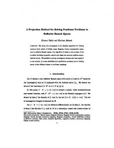
Consider the truss structure shown in Figure 1. The structure consists of 39 bars with stiffness and damping connecting 17 masses at the nodes. The dynamics of the structure can be and the state variable t written as i = Az where A E R64x64, consists of ( a linear combination) of the horizontal and vertical

1387

The full-order HAC controller is designed based on a reduced-order truss model, using the 5 lowest frequency modes. These are the most lightly damped modes and have a good frequency seperation from the remaining 27 modes. The eigenvalues of the feedback interconnection of the HAC (which is of order 10) and the truss are shown in the top of Figure 3 (only eigenvalues near the origin are shown). Note that, as a result of the spillover, the system is actually unstable and the eigenvalue-placement specification is obviously violated. At the second step of the design, t o satisfy the eigenvalue specifications, damping (limited in this case for illustrative purposes t o a maximum size of 0.08) is added along the bars. However, with the limited amount of damping allowed in this problem, the eigenvalue-placement specifications still cannot be achieved when all dampings are set t o the maximum of 0.08 (Figure 3). Therefore, besides adding damping along bars, we need t o adjust the HAC t o hopefully get a feasible solution. The problem of jointly designing the dampers and adjusting the HAC is a BMI which we will attempt t o solve using the path-following method of this paper.

displacements, and rates of displacements of each mass, ui, vz, iri respectively for i = 1,.. . ,17. This problem investigates a typical LAC application, which is to add modest damping to a structure to compensate for spillover from a higher-authority controller (HAC) that has been designed using a reduced model of the structure. The design methodology in this example follows the classic twostep process [16, 171. We first design a HAC, which is, for example, a Linear-Quadratic Gaussian (LQG) controller or a controller that achieves some eigenvalue-placement specification (note that the specific design process for the initial HAC is not important for this paper). A key point is that these higher authority designs are typically based on significantly reduced order models of the system to avoid designing a very high order controller. As a result, we would expect a considerable amount of spillover of the control authority to the higher frequency modes of the structure. The destabilizing effects of the spillover are addressed during the second step of the design by adding sufficient damping along bars. In this example it is required that the additional damping be such that the closed-loop eigenvalues fall within the shaded region of Figure 2 (corresponding to a minimum damping of 0.01 and minimum damping ratio of 0.02).

hi,and

h

E -4 -0.08

-007

-om

-005

-OM

-OM

-002

-001

a

001

-007

-om

-005

-004

-OM

-002

-001

a

001

I -008

I

Re(s)

Figure 1: Truss structure consists of 39 bars (stiffness and damping) and 17 nodes (masses).

3

,

-

2-

I

I

0

001

open-loop eigenvalues

1-

0-

1

-2

3

-005

-OM

-003

-002

-001

Figure 2: Open-loop eigenvalues of structure and the desired region for closed-loop eigenvalues.

Figure 3: Eigenvalues of the feedback interconnection of the truss and initial HAC with no dampers (top), and with all dampers set t o the maximum value of 0.08 (bottom). Clearly, eigenvalue specifications are not satisfied even when the dampings are maximum. In the framework considered in this paper, for the second step of the design, the open-loop system is actually the interconnection of the HAC and the truss. The variables in the design are the amount of damping along the bars as well as perturbations t o the elements of the HAC system matrices. The perturbations are limited t o 5% of their original values for first order perturbation formulas t o be approximately valid (the HAC is put in modal form). The problem specification is to minimize the sum of the damper values subject to the eigenvalue specifications. Using a path-following method for solving this BMI and first order perturbation formulas for the eigenvalues of a matrix [lo], at each iteration we need to solve a linear program (LP) with 419 variables and 483 linear inequality constraints. This can be readily done using widely available software for solving LPs' It turns out that after a single iteration of the pathfollowing method the eigenvalue-placement specification is lFor example the LP solver PCx can be downloaded from WWW at URL http://www-c.mcs.anl.gov/home/otc/Library/PCx/

1388

achieved (in other words the low-authority assumption is valid). The eigenvalue locations for the closed-loop system after adding the dampers and adjusting the HAC are shown in Figure 4. The figure clearly shows that this combined HAC/LAC design has sufficiently damped the (unstable) modes of the system. (Note that a couple of eigenvalues slightly violate the damping ratio constraint but we can simply perform another iteration t o fix this problem.) Figure 5 shows the location of the nonzero dampings. The total amount of damping added t o the structure in these 19 struts is 1.28 (this is less than the maximum amount of 39 x 0.08 = 3.12 tried before).

5 Conclusions

In this paper we presented a path-following method for (locally) solving BMIs. T h e method is very easy t o implement and is based on linearizing the BMIs and solving a sequence of SDPs. In general, as with all local methods for solving BMIs, the choice of initial value is important for convergence to a n acceptable solution. As long as the initial value is ['close enough" to the optimum value we expect the method to work well. However, the examples demonstrate that quite large performance improvements are possible using this method. It was also shown t h a t by minimizing the norm of feedback gains we can arrive at sparse designs, and therefore in effect, we can solve sensor/actuator placement and controller structure design problems. References

L. Vandenberghe and S. Boyd. SP: Software f o r Semidefinite Programming. User's Guide, Beta Version. Stanford University, October 1994. Available at (11

http://wwu-isl.stanford.edu/people/boyd. [2] S.-P. Wu and S. Boyd. SDPSOL: A Parser/Solwer for Semidef-

I

-om

-007

-om

-00s

-DM

-om

-002

-001

I

I

o

ooi

Re(s) Figure 4: Eigenvalues of the feedback interconnection of the truss and HAC before adding dampers ( t o p ) , and after adding dampers and adjusting the HAC (bottom).

/

............ a

-

\

Figure 5: Location of dampers for damper design for the feedback interconnection of the plant and the HAC. A solid line between two nodes corresponds t o a nonzero damper between those two nodes.

This simple problem shows t h a t there are often key advantages t o simultaneously designing the HAC and LAC components of the control architecture. More importantly, however, this example also shows that this entire control design problem can be posed as an LP, which can be solved very efficiently and very quickly on a simple computer.

inite Programming and Determinant Mazimization Problems with Matrix Structure. User's Guide, Version Beta. Stanford University, June 1996. [3] P. Gahinet and A. Nemirovskii. LMI Lab: A Package for Manipulating and Solving LMIs. INRIA, 1993. F. Alizadeh, J. P. Haeberly, M. V. Nayakkankuppam, and [4] M. L. Overton. SDPPACK User's Guide, Version 0.8 Beta. NYU, June 1997. [5] B. Borchers. CSDP, a C library for semidefinite programming. New Mexico Tech, March 1997. [6] K. C. Goh, M. G. Safonov, and G. P. Papavassilopoulos. A global optimization approach for the BMI problem. In Proceedings of the 33rd IEEE Conference on Decision and Control, December 1994. [7] K.-C. Goh. Robust Control Synthesis Via Bilinear Matrix Inequalities. PhD thesis, University of Southern California, May 1995. [8] M. Mesbahi, G. P. Papavassilopoulos, and M. G. Safonov. Matrix cones, complementarity problems and the bilinear matrix inequality. In Proc. IEEE Conf. on Decision and Control, pages 3102-3107, 1995. [9] E. Beran, L. Vandenberghe, and S. Boyd. A global BMI algorithm based on the generalized Benders decomposition. In Proceedings of the European Control Conference, July 1997. [lo] A. Hassibi, J. How, and S. Boyd. Low-authority controller design via convex Optimization. In Proc. IEEE Conf. on Decision and Control, December 1998. [ll] A. Hassibi, J. How, and S. Boyd. Low-authority controller design via convex optimization. AIAA J. Guidance, Control, and Dynamics, 1998. Submitted. (121 V.D. Blonde1 and J. N. Tsitsiklis. NP-hardness of some linear control design problems. SIAM J. on Control and Optimization, 35:2118-27, 1997. [13] S. Boyd, L. El Ghaoui, E. Feron, and V. Balakrishnan. Linear Matrix Inequalities in System and Control Theory, volume 15 of Studies in Applied Mathematics. SIAM, Philadelphia, PA, June 1994. [14] A. Nemirovskii. Several NP-Hard problems arising in robust stability analysis. Mathematics of Control, Signals, and Systems, 6(1):99-105, 1994. [15] P. P. Khargonekar and M. A. Rotea. Mixed ' H z / ' H , control: A convex optimization approach. IEEE Fmns. Aut. Control, 36(7):824-37, July 1991. [16] 3 . N. Aubrun. Theory of control of structures by lowauthority controllers. J. Guidance and Control, 3(5):444-451, September 1980. [17] J. N. Aubrun, N. K. Gupta, and M. G. Lyons. Large space structures control: An integrated approach. In Proc. AIAA Guidance and Control Conference, Boulder, Colorado, August 1979.

1389