Computer Graphics, 26,2, July 1992
A Physically
Based
Approach Thomas
W.
Eugene Brigham
Shape Blending
Sederberg
Greenwood Young
Abstract This paper presents a new afgorithm for smoothly blending between two 2-D polygonal shapes. The algorithm is based on a physical model wherein one of the shapes is considered to be constructed of wire, and a solution is found whereby the first shape can be bent and/or stretched into the second shape with a minimum amount of work. The resulting solution tends to associate regions on the two shapes which look alike. If the two polYgons have m and n vertices respectively, the afgorithm is O(mn). The algorithm avoids local shape inversions in whkh intermediate polygons self-intersect, if such a solution exists. Categories and Subject Descriptors: 1.3.3 [Computer Graphics]: Picture/Image Generation; 1.3.5 [Computer Graphics]: Computational Geometry and Object Modeling. General Terms: Algorithms Additional Key Words and Phrases: Computer graphics, shape blending, animation, physically based algorithms.
1
to 2–D
University
-5
FF
Figure 2: Shape blend example
two polygonal shapes, the problem is to compute a continuous shape transformation from one to the other. For example, in Figure 1, the far left and far tight sketches of a chicken are given, and the three intermediate shapes are automatically computed with no user interaction. This operation is known variously as shape averaging, shape interpolation, metamorphosis, shape evolving, and shape blending. It has widespread application in illustration, animation, and industrial design. 2-D shape blending is an increasingly popular feature in man ~;~;;;ial illustration software packages (such as [1], [6], [7%
Introduction
The topic of this paper is illustrated
in Figures
-3.
Given
Figure 3: Shape blend example
Figure
Solutions to the 3-D shape interpolation problem have also been proposed ([4], [1o], [14]). Indeed, the research effort reported in this paper initially focused on the 3–D problem. However, the authors soon realized that even the 2-D problem had many open questions, such a how can a shape blend algorithm avoid chaotic intermediate shapes and how can an
1: Shape blend example
] Engineering Computer Graphics Laboratory 368 Clyde Building Brigham Young University Provo, UT 84602 801 378-6330 H801 378-2478
FAX
[email protected]
AcM-o-x97Yl-479
-l/92 /(M)7/cQ25
$01 so
25
SIGGRAPH ’92 Chicago, July 26-31, 1992
algorithm recognize similar, t bough not identical, features on the two terminal shapes (such as the feet and head of the chicken in Figure 1) and maintain those features throughout the blend. We tested several commercial shape blending software packages on some of our shape examples. The best of any results for the chicken outline is shown in Figure 4 and the best E to F blend is shown in Figure 5. Notice how the chicken feet in Figure 4 degenerate to a self-intersecting scribble.
Figure 6: Family of blend polygons
Figure 4: Shape blend of chicken using commercial
software
EEFFFF Figure 5: Shape blend of E to F using commercial
software
The algorithm presented in this paper is baaed on a physical model. Imagining that each shape is made of a piece of wire, the blend is determined by computing the minimum work required to bend and stretch one wire shape into the other. The user can specify some physical properties of the wire, which control the relative difficulty with which it can be bent or stretched. A severe penalty is charged for blends which experience a local self intersection due to the wire bending through an angle of zero degrees. This penalty nearly always prevents the self intersection problem in Figure 4. AU of the blends in this paper were generated automatically with no user intervention (Figures 4 and 5 by commercial packages, the rest by our algorithm) except for initially specifying the physical attributes of the wire.
1.1
Related
work
Shape blending is a problem which has been motivated by several different applications and attacked in several different ways. For example, if we envision the family of blend polygons aa formin a ruled surface in (z, y, t) space, as shown in Figure 6, the sf ape blending problem bears strong similarity to the contour triangulation problem [5], [8], [9], [15]. This is the background from which we approached the problem, and our solution borrows graph theory concepts from [15] and [8]. The algorithms used in the commercial illustration software cited above probably resemble the triangulation algorithms in [5] and [9] since these are O(n) in time and memory, thus more suitable for PC applications than ones based on raph theory. The first paper on 3-D shape interpolation 4] was motivated by industrial design. It tackles the pro [ Iem by slicing the two 3–D shapes into contours, blendlng corresponding contours, then reconstructing the 3–D blended surface. More recent solutions, [10] and [147 , are based on Minkowski sums. These approaches give impressive results, but leave some room for further investigation. For example, two non-convex objects 26
as a function
oft
with similar features (such aa a dog and a horse) will lose protruding detaUs such as legs during intermediate shapes. In fact, the blend of a non-convex object with itself is not a constant shape. Problems related to 2–D shape blending arise in shape recognition [2], [19] and curve matching for graphical search and replace [16 . In these applications, the primary concern is determining Low similar two complete objects are. Shape blending also resembles the computer vision problem of contour identification, for which one solution is based on energy minimization [13], as is the shape blendhg algorithm described herein. When the two shapes to be blended are taken to be key frames in a character animation (such as in Figure 1) shape blending is similar to inbetweening — an important component of the general problem of computer-assisted animation [3). The problem addressed in this paper, inbetweening of poly onal shape outlines, is simpler than the more general prob f em of inbetweening complete drawings.
1.2
Overview
Section 2 discusses geometric aspects of the shape blending problem. The physical work model is discussed in section 3. The minimum work solution is found by means of a directed graph, as discussed in section 4. Section 5 presents several examples and discusses the relative influence of stretching and bending work.
2
Geometric
preliminaries
Given two polygons P. and PI with the same number of vertices, shape blending is accomplished by performing a linear interpolation between the corresponding vertices of the two polygons. If PO=[P:,
Pf,...,
P:];
where P! denote vertices, can be defined P(t)
=
P1 =[P~,
intermediate
P;,...,
P:]
(1)
polygons in the blend
uPO + tP1
=
[uP:+tP;,
=
[P~(t), P~(t),
uP;
+tP;
,.. ,Pn(t)]
,,..,
uP:
+tP:] (2)
where u = 1 -t. The motion of three adjacent vertices undergoing a shape blend is shown in Figure 7. Consider the simple example in Figure 8, where the vertex numbers are labeled. Each intermediate shape is determined by linearly interpolating each node as shown. The paths for vertices 1 and 3 are shown in dotted lines.
Computer Graphics, 26,2, July 1992
B:
izllixY211 ‘225’’’’+’(0)
//–’
“,
P&q.l (o)
\.
\
(.5)
B}
.
pl
“y+1(,5) Figure
/
+(1) ~,, ; 11
.
q.l(.i
po
“ Pi(.5)
solution
3
ii21151iT3f
I+Pi+l(l) q(l)
P:~Pi., (;; ‘ P
po
pl
Figure Figure 7: Blending
10: Simple example,
of three adjacent
11: Simple example,
solution
4
vertices vertex pass over one another. When this happens, at least part of the sha~e is turnin~ itself “inside out”. Another ex;mple of ii-behaved intermediate angles is shown in Figure 13. Here, the terminaf angles at vertices 4 and 6 are both 90°, yet those angles in the intermediate blends exceed 130°. Also, vertex 5 begins and ends on a straight line, yet that line becomes noticeably bent during the blend operation. Figures 12 and 13 suggest two angle constraints that should be imposed on blend solutions. First, if at all possible we should avoid Oi(t) = O O