JOURNAL OF COMPUTERS, VOL. 4, NO. 8, AUGUST 2009
787
A Practical Dynamic Frequency Scaling Solution to DPM in Embedded Linux Systems Zhang YuHua School of Computer Science and Technology,Soochow University, Suzhou, China Email:
[email protected]
Qian LongHua,Lv Qiang, Qian Peide,Guo Shengchao School of Computer Science and Technology,Soochow University, Suzhou, China Email: {Qianlonghua,qiang}@suda.edu.cn
Abstract—Traditional power management enables CPU to switch among different power consumption modes such as running, idle and standby to save energy to a certain degree. In battery-powered embedded Linux systems, power management plays an even more important role than in desktops. This paper proposes a practical solution to dynamic power management (DPM) based on dynamic frequency scaling (DFS). According to the system workload, it switches the working frequency among several predefined settings. This paper presents a design and implementation of the solution in an embedded Linux system. Experimental results on an Intel PXA250-based system have demonstrated that the system running a DPM-enabled Linux can save up to 44% of execution time with less than 8% extra power consumption in an email application. Index Terms—Dynamic Frequency Voltage Scaling, Embedded Linux
Scaling,
Dynamic
I. INTRODUCTION With recent popularity of mobile computing, power management scheme becomes an important concern in embedded applications. In portable, battery-powered devices such as personal digital assistants and mobile phones, effective and efficient power management scheme can reduce power consumption of the embedded applications, and extend their working hours as long as possible to satisfy users’ need of portability and durability. On the other hand, as an embedded system usually comprises of high density of millions of transistor gates, if the device often runs at a high temperature caused by excessive power consumption without appropriate cooling components, it will surely do harm to the reliability and lifetime of the embedded system. Traditional power management module can switch CPU among different power consumption modes, e.g. running, idle and standby etc., to save energy as much as possible. When CPU has no job to run, it will be put into the idle mode. At that time its core clock stops working, but the components that monitor various interrupt requests are still in active state so as to keep the system states of both software and hardware. As soon as one of the interrupt requests arrives, the CPU is pulled back to the running mode. Such switching between running and idle modes is easy to implement, but the energy savings it brings about are limited. Further, if the idle time is © 2009 ACADEMY PUBLISHER
greater than a threshold, the system will be set to the standby mode until it is waked by user’s keystroke or other events. In this mode, the power of most components is off except the one that detects the signal of waking the standby mode, thus the switching between running and standby modes is relatively complex, but the consequence of this functionality greatly reduces the power consumption. As a matter of fact, during the running mode the system workload varies from time to time. If the power consumption is reduced when the workload is low, then the overall energy consumption of the embedded system can be further decreased. Dynamic power management (DPM) [1,2,3] can adjust the hardware working status according to the system workload. Dynamic voltage scaling (DVS) is a known effective mechanism of DPM for reducing CPU energy consumption without degrading system performance significantly. When the system workload is lower, the CPU voltage will be decreased to reduce the power consumption. When the system workload becomes higher, the CPU voltage will be increased to shorten the user response time. However, the implementation of DVS in an embedded system is really an intractable task for its workload measurement and voltage switching [3,8,10,11]. This paper proposes a practical solution to DPM based on dynamic frequency scaling (DFS). According to the system workload, it switches the working frequency among several predefined settings. We carefully designed and implemented this solution in an embedded Linux system. Experimental results on an Intel PXA250-based system have demonstrated that the system running a DPM-enabled Linux can save execution time with little extra power consumption in an email application. This paper is organized as follows. Section II introduces related work of DPM and motivation of our approach. It then elaborates the design of DFS solution in the embedded Linux system based on Intel PXA250 microprocessor. Section Ⅲ explains how to implement this solution, including measuring the system workload in an approximately fixed interval, followed by speed controlling scheme based on the three consecutive sampling results of the system workload. Experimental results of system boot up are analyzed in Section Ⅳ, and energy savings in an email application brought about by
788
JOURNAL OF COMPUTERS, VOL. 4, NO. 8, AUGUST 2009
DFS solution are also discussed in this section. Finally SectionⅤprovides our conclusions and future discussions. II. DYNAMIC FREQUENCY SCALING A. Background and Related Work DVS was elaborated from a theoretical perspective in [9]. The main source of power dissipation in a digital CMOS circuit of the embedded system is the dynamic power dissipation: M
2 Pdynamic = ∑ CLk • Switk • VDD
(1)
k =1
where M is the number of the gates in the circuits, CLk is the load capacitance of the gate gk, Switk is the switching speed of the gate gk, and VDD is the supply voltage. However, reducing power supply causes increase of circuit delay. The circuit delay is estimated by the following formula: τ∝ VDD /(VG -VT )2 (2) where τ is the propagation delay of the CMOS transistor, VT is the threshold voltage, and VG is the voltage of the input gate. (1) and (2) indicate that there is a fundamental tradeoff between the switching speed and the supply voltage. When the supply voltage decreases to reduce the power consumption, the switching speed also must be decreased to tolerate the increased propagation delay. We recast the equation as the following one, assuming that the dynamic power is the most dominant one: 2 P = C • f • VDD
(3)
This equation shows that the power consumption is linearly proportional to clock frequency and square of supply voltage. Accordingly, one can reduce power consumption by reducing these two variables. Furthermore, by reducing the supply voltage, one also increases a circuit’s delay linearly. The switching speed will be lower accordingly, that reduces the power consumption intensively. This is called dynamically voltage scaling (DVS). The motivation behind DVS is that actively scheduling tasks running speed, higher or lower, can save energy. However, system performance will degrade if clock frequency is lowered, and the time to complete a task will increase. So there is a trade-off between the power consumption and the system response time to the user. Scaling the supply voltage means scaling the working frequency accordingly. From another perspective, to every working frequency, there should be a corresponding lowest supply voltage to support this working frequency properly while minimizing the power consumption. Dynamic frequency scaling (DFS) is used to adjust the working frequency according to the system workload in order to save the power consumption without degrading the system performance significantly beyond the user tolerance. In fact DFS is a variant of DVS, but here the focus is the working frequency, which is closely
© 2009 ACADEMY PUBLISHER
related to the response time in the whole system-level. Only when the decrease of the working frequency doesn’t affect the response time significantly, can we lower the working frequency and the corresponding supply voltage to get energy savings. Early related work on DPM includes theoretical studies [9] and simulations on the potential of DVS techniques [7, 8, 10]. Since then, practical implementation of DVS schemes have already been proved feasible with some commercial processors [1, 18] and academic design efforts [11, 12, 16]. Various DPM models are also proposed to scale voltage with underlying software support [13,14,15,17,19,20]. These works focus on model-based complex DVS algorithms, relatively few are on the practical solutions to implement them in a real embedded system. Another aspect is that most of these related works concentrate on frequency scheduling or energy savings of individual components, e.g. CPU, memory ,disk [21,22,23] etc. Seldom are on system-level energy savings. One of the motivations that distinguish our work from previous research is that we design and implement a practical solution to DPM in a real embedded Linux system based on Intel PXA250 microprocessor. The ready statistics data source provided by the kernel is utilized to compute the workload trend. PXA250 also provides easily customized one-step operation to frequency scheduling based on mode switching. Another objective is that frequency scheduling is not limited to individual component (usually CPU); we can also optimize the memory frequency in accordance with one designated CPU frequency. Finally we evaluate our solutions through the overall system-level energy saving brought about by DFS in a real system running an email application recursively. B. Design of DFS in PXA250 Figure.1 describes the dynamic power management model with DFS. It consists of a monitor and a controller of the system. The monitor checks the current system running status to get the information about the system workload, and reports the workload information to the controller. The controller switches the working frequency according to the dynamical trend of the system workload. If the system workload rises, then working frequency is increased to shorten the response time. Vice verse, if the system workload drops, the working frequency is decreased to save the power consumption. Through careful design of workload monitoring and speed controlling, we can reach an optimal balance between lowest power consumption and tolerable response time. There are two key problems in DFS solution. One is how to detect the system workload trend. The other is how to switch the working frequency as quickly as possible. Both of these computation and switching operations should not take much time to degrade the system performance and consume extra power, so we need efficient and effective solutions. As for the first one, we apply a simple yet practical method to determine the workload trend as detailed in Section Ⅲ. On the other hand, the PXA250 microprocessor provides easily
JOURNAL OF COMPUTERS, VOL. 4, NO. 8, AUGUST 2009
customized switching functionality to solve the second problem. Workload Monitor
workload information
running information
Speed Controller
control commands
System
Figure 1. dynamic power management model
The hardware platform of our target embedded system is an Intel PXA250-based system with X-Scale architecture [6] and PXA250 microprocessor. The PXA250 microprocessor provides effective and efficient DFS support to DPM. In this microprocessor the working frequency is mainly controlled by core clock configuration register (CCCR). By setting the different value of CCCR, the working frequency of RAM and CPU can be dynamically adjusted accordingly. However, Intel Corporation doesn’t suggest this solution for the sake of operation complexity and system safety. During the period of system running, modifying frequency multiplier coefficients dynamically covers a sequence of very complex operations that inevitably incur relatively great time delay. Further more, most of the system components and peripherals will be affected during that time. In order for developers to adjust the working frequency safely and quickly, Intel supplements an additional Turbo running mode for PXA250 besides the normal Running mode. It is suggested that proper frequency multiplier coefficients of CCCR be set when the system is initialized. Therefore DFS can be achieved by switching CPU running modes between normal and turbo modes very quickly when the system is running [4]. The working frequency of both PXA250 and memory are derived from a crystal oscillator with 3.6864MHz frequency. CCCR defines frequency multiplier coefficients L, M and N between CPU and the crystal oscillator. Memory Frequency = Crystal Frequency * L Run Mode Frequency = Memory Frequency * M Turbo Mode Frequency = Run Mode Frequency * N Where L is Crystal Frequency to Memory Frequency Multiplier, M is Memory Frequency to Run Mode Frequency Multiplier and N is Run Mode Frequency to Turbo Mode Frequency Multiplier. The microprocessors with Intel X-Scale architecture may support CPU working frequency with very wide range, but the stable frequency range for PXA250 is limited from 100MHz to 400MHz. According to the suggestion from Intel Corporation, the CPU mode is switched between the Running mode and the Turbo mode so as to adjust the CPU working frequency dynamically. When CPU is initialized through Boot Loader module in embedded Linux, the frequency multiplier coefficients are set to L (27), M (2) and N (2). As the result of this © 2009 ACADEMY PUBLISHER
789
setting the frequency of memory, the Running mode and the Turbo mode is 100MHz (99.53≈100), 200MHz and 400MHz respectively. When the system is running, the system workload is computed and compared periodically. If the workload is increasing, switch the CPU from the Running mode to the Turbo mode in order to make it run with 400MHz. On the contrary, if the system workload is decreasing, then switch it from the Turbo mode to the Running mode in order to make it run with 200MHz. III. IMPLEMENTATION ISSUES In order to implement DFS in embedded Linux based on Intel PXA250, first we should detect the system workload trend as precise as possible. This step starts with the determination of an approximately fixed interval (100ms), then computes the idle time proportion in this interval periodically, and finally compares the three consecutive results to judge the workload trend. The last implementation issue is the switching functionality of the working frequency. Switching the working frequency is absolutely not an easy work while the system is running. However, in Intel PXA250 because the system has set all the values in CCCR related to DFS when it starts up, what we want to do is to only reverse the Turbo bit in the coprocessor register CCLKCFG to switch the working frequency. A. Workload Measurement Scheme The first problem of DFS solution is how to compute the system workload trend. That’s a critical problem, for the computation cost of complex detection algorithms will probably dwarf the advantage of energy saving by DFS. Weiser, et al. [8] proposed three scheduling algorithms to predict the future workload, namely OPT, FUTURE and PAST. The goal of these algorithms is to decrease time wasted in the idle loop while retaining tolerable interactive response. OPT spreads computation over the whole trace period to eliminate all idle time, and FUTURE uses a limited future look ahead to determine the minimum clock. Both of OPT and FUTURE algorithms need future knowledge to compute the system workload trend. This is impractical in most running system, because it’s hard to know the future workload exactly, so these two algorithms are only suitable for the simulation system [8,9,10] or a baseline system for comparison, while the PAST algorithm looks a fixed window back into the past workload, and assumes the next window will be like the previous one. Although it is not always true that the next window will be like the previous one, we can get the previous workload information relatively easily, so this algorithm is really a simple and practical one. Thereafter, Govil et al. [7] used a more sophisticated predication method in order to improve performance substantially. As for the simplicity of implementation and availability of workload information, we adopted the simplified elementary PAST algorithm described as the following. Linux kernel we constructed based on PXA250 microprocessor provides statistics data sources related to the system workload through /proc file system. One is
790
JOURNAL OF COMPUTERS, VOL. 4, NO. 8, AUGUST 2009
located in the system directory /proc/loadavg which computes the number of processes in TASK_RUNNING state over the past 1, 5, and 15 minutes to reflect system busyness. The other is the cpu data item in the directory /proc/stat which provides the ticks that the CPU is in user mode, kernel mode and idle mode respectively since the system is started up. Because the time interval for the first method to compute the workload is too long, while the second one can reflect the system workload trend as precise as possible, we think the second one is more appropriate. If in a fixed interval the proportion of the idle time to total time becomes higher, it is supposed that the system is idler than before. On the contrary, the system will be busier than ever. Based on this consideration and the workload computation method used in DPM in Windows CE [5], we propose the following algorithm. The proportion of the idle time is first computed periodically. Then three consecutive results are compared. The computation procedure can be expressed as the following formulas: T _ per ≈ 100ms M
(4)
T _ idle = ∑ T _ idlek
(5)
T _ rate = T _ idle / T _ per
(6)
k =1
where T_per is the sampling interval (empirically approximate 100ms [5]), T_idle is the accumulated idle time in T_per, T_rate is the proportion of the idle time T_idle to T_per, and one of the sampling results we want. Judging by comparing three consecutive results, if T_rate1 < T_rate2 < T_rate3, we think the system workload is decreasing, lower the speed then; if T_rate1 > T_rate2 > T_rate3, the system workload is increasing, raise the speed.
B. Sampling Interval Determination The first of workload computation is determination of the sampling interval. The clock framework in Linux kernel provides appropriate solution to determine the sampling interval. Just like in X86 platform, the timing device in PXA250 will trigger the clock interrupt in every 10 milliseconds, then the interrupt routine do_timer() in kernel/timer.c will be called. Fig. 2 depicts the flow chart of sampling interval determination that we use. The routine do_timer() first increases the global variable jiffies by one, where jiffies records clock ticks (1 tick=10ms) since startup of the system. Then it refreshes the kernel global variable kstat that records many pieces of kernel statistics information through update_process_times(). Linux kernel executes the routine do_timer() 100 times in every 1 second, so this routine cannot do too many things, the other important works should be done in bottom-half process. In the final stage the routine do_timer() activates bottom-half routine timer_bh(), and the kernel will run timer_bh() in the appropriate time. The bottom-half processing can be finished in 1 tick when the workload is light. However, when the workload is heavy, the bottomhalf routine will probably run one time in several ticks. As a result, the sampling interval may be a little bit greater than T_per. The timer_bh() calls the routines update_times() and run_timer_list() respectively. The first one is used to refresh system wall clock and the second one is used to run tasks in the kernel timer queue. Here we only concern update_times(). In the routine update_times(), the sampling interval is initialized to zero and accumulated by ticks. When the sampling time reaches 100 milliseconds, the routine calc_idle_rate() will be called to compute the system workload trend, and the CPU working frequency will be adjusted if needed.
update_times
do_timer
update_system_ wall_clock
jiffies=jiffies+1
mark_bh(TIMER_BH) update_process_times
compute_workload_ information
update_times sampling interval>=100ms?
mark_bh(TIMER_BH) run_timer_list
calc_idle_rate
End
Figure 2. the flow chart of sampling interval determination
© 2009 ACADEMY PUBLISHER
JOURNAL OF COMPUTERS, VOL. 4, NO. 8, AUGUST 2009
C. Workload Measurement Implementation The main task of routine calc_idle_rate() as illustrated in Fig. 3 is to compute the proportion how much the idle time is in the fixed time T_per. One direct method is to sum the intervals every time when CPU is in idle mode. Because of its computation cost, this is not a practical method. What we use is an indirect method. The kernel global variable kstat records the time when it is in user mode and system mode in kstat.per_cpu_user[cpu],
791
kstat.per_cpu_nice[cpu] and kstat.per_cpu_system[cpu] (cpu is always zero when there is only one processor) respectively, and the sum of these items is just the time when CPU is running. We subtract this sum from the interval T_per to get the accumulated idle time. This method utilizes the ready kernel statistics information to compute the idle time, and avoids computing the sum every time when CPU enters the idle mode, so it needs lower computation cost than the first one.
calc_idle_rate
compute the time when CPU is in running mode
the workload rise?
compute one of the three percentage rate[i]
sampling times reach three?
Y
N
the workload decrease?
N
Y
switch from Running to Turbo
Y
switch from Turbo to Running
N
End
Figure 3. workload measurement and speed controlling
After the three consecutive results have been sampled, we compare these results. If rate1>rate2>rate3, then switch the CPU from the Running mode to the Turbo mode. Vice verse, if rate1