A Probabilistic Framework for Feature-based Speech ... - CiteSeerX

A PROBABILISTIC FRAMEWORK FOR FEATURE-BASED SPEECH RECOGNITION1 James Glass, Jane Chang, and Michael McCandless Spoken Language Systems Group Laboratory for Computer Science Massachusetts Institute of Technology Cambridge, Massachusetts 02139 USA

ABSTRACT Most current speech recognizers use an observation space which is based on a temporal sequence of “frames” (e.g., Mel-cepstra). There is another class of recognizer which further processes these frames to produce a segment-based network, and represents each segment by fixed-dimensional “features.” In such feature-based recognizers the observation space takes the form of a temporal network of feature vectors, so that a single segmentation of an utterance will use a subset of all possible feature vectors. In this work we examine a maximum a posteriori decoding strategy for feature-based recognizers and develop a normalization criterion useful for a segmentbased Viterbi or A search. We report experimental results for the task of phonetic recognition on the TIMIT corpus where we achieved context-independent and context-dependent (using diphones) results on the core test set of 64.1% and 69.5% respectively.

1.

INTRODUCTION

The SUMMIT speech recognizer developed by our group uses a segment-based framework for its acoustic-phonetic representation of the speech signal [22]. Feature vectors are extracted both over hypothesized segments and at their boundaries for phonetic analysis. The resulting observation space (the set of all feature vectors) takes the form of an acoustic-phonetic network, whereby different paths through the network are associated with different sets of feature vectors. This framework is quite different from prevailing approaches which employ a temporal sequence of observations. The segmental and feature-extraction characteristics of this recognizer provide us with a framework within which we try to incorporate knowledge of the speech signal. They enable us to explore different strategies for where to extract information from the speech signal, and allow us to consider a larger variety of observations than we could with traditional frame-based observations. We have always tried to cast the recognizer within a probabilistic framework in order to account for our incomplete knowledge. We have been troubled, however, that different paths through our segment-network compute likelihoods on essentially different observation spaces (different segments have different feature vectors), 1 This research was supported by DARPA under contract N66001-94-C-

6040, monitored though Naval Command, Control and Ocean Surveillance Center. J. Chang receives support from Lucent Technologies.

yet our decoder compares the likelihoods of each path to decide on the most-likely word sequence. Additionally, while we train models based on positive examples of our lexical units (e.g., phones), we compute and rank model likelihoods on segments which are not valid units during decoding. This problem is especially serious if likelihoods are converted to posterior probabilities, since a poor likelihood could result in a very good posterior probability only because it happens to be a little better than the (positive) alternatives. Recently we have reexamined the probabilistic framework we have been using and have adopted a new strategy which we believe better accounts for our feature-based observation space, is intuitively appealing, and reduces the number of tuning parameters required by our system. We now utilize the entire network of hypothesized segments (both positive and negative examples) during training, and try to account for the entire observation space during decoding. In this paper we show how we derived this framework from basic MAP decoding principles, and present a normalization criterion which can be used to implement efficient decoding for a featurebased recognizer. We then report experimental evidence on phonetic recognition which we have used to evaluate the framework.

2. MAP DECODING In most probabilistic formulations of speech recognition the goal is to find the sequence of words W  = w1 ; : : : ; wN , which has the maximum a posteriori (MAP) probability P (W A), where A is the set of acoustic observations associated with the speech utterance:

j

W  = arg max P (W jA) W

In most speech recognizers, MAP decoding is accomplished by hypothesizing (usually implicitly) a segmentation S of the utterance into a connected sequence of lexical states or units. In these cases P (W A) can be rewritten as

j

P (W jA) =

X P (WSjA)  max P (WSjA) S

S

The latter approximation assumes that there is a single “correct” segmentation S  associated with W  . This approximation simplifies the decoding process by allowing the use of dynamic programming algorithms which seek only the “best” path (e.g., Viterbi, or A ).

jA) is typically converted to the form: P (WS jA) = P (ASPjW(A))P (W ) Since the denominator is independent of S or W , it is usually ignored during decoding. The remaining terms P (AS jW ) and P (W ) The expression for P (WS

a1

j

2.1. Frame-based Observations Most speech recognizers take as input a temporal sequence of vectors or frames, O = o1 ; : : : ; oT , which are normally computed at regular time intervals (e.g., 10 ms). In most cases a frame contains some form of short-term spectral information (e.g., Mel-cepstra). When the observation space consists of a sequence of frames, A = O, and acoustic likelihoods are computed for every frame during decoding. Thus, the term P (A SW ) accounts for all observations, and competing word hypotheses can be compared directly to each other since their acoustic likelihood is derived from the same observation space. Note that by definition A includes all observations so the denominator term P (A) can be ignored.

f

g

j

As mentioned previously, most recognizers use frame-based observations for input to the decoder. Thus all discrete and continuous HMMs, including those using artificial neural networks for classification, fit under this framework [7, 12, 15, 16, 21]. Many segmentbased techniques also use a common set of fixed observation vectors as well. Marcus for example, predetermines a set of acousticphonetic sub-segments, represents each by an observation vector, which is then modelled with an HMM [11]. Other segment-based techniques hypothesize segments, but compute likelihoods on a set of observation frames [2, 6, 10, 19].

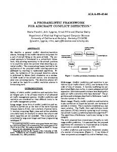
2.2. Feature-based Observations In contrast to frame-based approaches, in a feature-based framework, each segment si is represented by a single fixed-dimensional feature vector xi . Typically, there is an extra stage of processing to convert the frame sequence O to corresponding features. Explicit segment or boundary hypotheses are necessary to compute the feature vector. A given n unit segmentation S = s1 ; : : : ; sn will have a set of corresponding n feature vectors X = x1 ; : : : ; xn . As illustrated in Figure 1, the observation space is transformed from a temporal sequence to a network, where different segmentations of the utterance will be associated with different feature-vectors. Since alternative segmentations will consist of different observation spaces, it is incorrect to compare the resulting likelihoods directly. In order to compare two paths we must consider the entire observation space. Thus, in addition to the feature vectors X associated

a4

a1

a3

j P (AS jW ) = P (AjSW )P (S jW )

where P (S W ) determines the probability of a particular segmentation (e.g., the HMM state sequence likelihood). P (A SW ) determines the likelihood of seeing the acoustic observations given a particular segmentation (or state sequence).

a5

a2

are usually estimated separately by acoustic and language models, respectively. In many formulations, such as hidden Markov models (HMMs), the term P (AS W ) is further decomposed into

j

a3

a5 a4

a2

Figure 1: Two segmentations through a segment network with associated feature vectors a1 ; : : : ; a5 . The top path uses vectors a1 ; a3 ; a5 , while the bottom path uses a1 ; a2 ; a4 ; a5 .

f

f

g

g

f

g

with the segmentation S , we must consider all other possible feature vectors in the space Y , corresponding to the set of all other possible segments R. In the top path in Figure 1, X = a1 ; a3 ; a5 , and Y = a2 ; a4 . In the bottom path, X = a1 ; a2 ; a4 ; a5 , and Y = a3 . The total observation space A, contains both X and Y , so for MAP decoding it is necessary to estimate P (XY SW ). Note that since S implies X we can say P (XY SW ) = P (XY W ).

f f g

g

f

f

j

j

g

g

j

In practice, most feature-based recognition systems have not estimated a probability for P (XY W ) but have only estimated the likelihood of X , P (X W ) [4, 9, 13, 22]. The following section discusses one method for estimating P (XY W ) in an efficient manner.

j

j

j

3. MODELLING NON-LEXICAL UNITS

j

One approach to modelling P (XY W ) is to add an extra class to the lexical units which is defined to map to all segments which do not correspond to one of the existing units. Consider the case where acoustic-modelling is done at the phonetic level, so that we build probabilistic models for individual phones,  . In this approach we can view the the segments in R as corresponding to the extra antiphone class   . This class contains all types of sounds which are not a phonetic unit as they are either too large, too small, or overlapping etc. Two competing paths must therefore account for all segments, either as normal acoustic-phonetic units or as the anti-phone  . In the example shown in Figure 1, the top path therefore would map feature vectors a2 ; a4 to   , whereas the bottom path would only map feature a3 to  .

f g

f f g

g

We can avoid classifying all the segments in the search space by recognizing that P (XY  ), the probability that all segments are not a lexical unit, is a constant K , and has no effect on decoding. Assuming independence between X and Y , noting that P (Y W ) depends only on  , we can decompose and rearrange P (XY W )

j

j

j

j) P (X jW ) P (XY jW ) = P (X jW )P (Y j ) PP ((X X j) = K P (X j )

Thus, when we consider a particular segmentation S we need only concern ourselves with the NS feature vectors corresponding to S , but we must combine two terms for each segment si . The first term is the standard phonetic likelihood P (xi ). The second term is the likelihood that the segment is the anti-phone unit, P (xi  ). The net

j

j

Y P (x jW ) P (s jW )P (W )

result which must be maximized during search is:

W  = arg max W;S

N

S

i=1

i

P (x j)

i

i

Note that this formulation remains the same whether contextindependent or context-dependent modelling is used. The term P (xi W ) would be reduced accordingly.

j

4.

MODELLING LANDMARKS

In addition to modelling segments, it is often desirable to provide additional information about segment boundaries, or landmarks. If we call the feature-vectors extracted at landmarks Z , we must now consider the joint space XY Z as our observation space. It thus becomes necessary to estimate the probability P (XY Z SW ). If we assume independence between the feature vectors XY representing segments and Z representing landmarks, we can further simplify:

j

P (XY Z jSW ) = P (XY jSW )P (Z jSW ) If Z corresponds to a set of observations taken at landmarks or boundaries, then a particular segmentation will assign some of the landmarks to transitions between lexical units, while the remainder will be considered to occur internal to a unit (i.e., within the boundaries of a hypothesized segment). Since any segmentation accounts for all of the landmark observations Z , there is no need for the normalization criterion discussed for segment-based feature vectors. If we assume independence between the NZ individual feature-vectors in Z , P (Z SW ) can be written as

j

Y P (Z jSW ) = P (z jSW ) N

Z

i

i=1

where zi is the feature vector extracted at the ith landmark. Again, there is no assumption about whether context-independent or context-dependent (diphone) boundary models are used.

5. EXPERIMENTS Our initial evaluations of this framework were based on phonetic recognition experiments using the TIMIT corpus [3]. Models were built using the TIMIT 61 label set and collapsed down to the 39 labels used by others to report recognition results [4, 7, 8, 14, 15, 21]. Models were trained on the designated training set of 462 speakers, and results are reported on the 24 speaker core test set. A 50 speaker development set (taken from the remaining 144 speakers in the full test set) was used for intermediate experiments so that the core test set was used only for final testing. Reported results are phonetic accuracy which includes substitution, deletion, and insertion errors. The language model used in all experiments was a phone bigram based on the training data with perplexity 15.8 on the development set (using 61 labels). A single parameter (optimized on the development set) controlled the trade-off between insertions and deletions. All utterances were represented by 14 Mel-scale cepstral coefficients (MFCCs) and log energy, computed at 5 msec intervals. Acoustic landmarks were determined by looking for local maxima in spectral

change in the MFCCs [22]. Segment networks were created by fully connecting landmarks within acoustically stable regions. An analysis of the networks showed that on the development set there were 2.4 boundaries per transcription boundary and 7.0 segments per transcription segment on average. Our research was greatly facilitated by SAPPHIRE , a graphical speech analysis and recognition tool based on Tcl/Tk that is being developed in our group [5]. S APPHIRE ’s flexibility and expressiveness allows us to quickly test novel ideas and frameworks.

5.1. Context-Independent Recognition The first set of experiments we performed used 62 labels (61 TIMIT labels plus the anti-phone “not”) to explore context-independent (CI) phonetic recognition using segment-based information only. The feature vector consisted of MFCC and energy averages over segment thirds as well as two derivatives computed at segment boundaries. Duration was also included, as was a count of the number of internal landmarks in the segment. The resulting segment feature vector contained 77 dimensions. Mixtures of up to 50 diagonal Gaussians (400 for the anti-phone) were used to model the phone distributions on the training data. An initial principal components analysis (PCA) was done to normalize the feature space for the mixture generation (which uses K-means clustering as an initial step), though no dimensionality reduction was done. In order to reduce training computation, 20% of the possible anti-phone examples were randomly selected to train the anti-phone model. The CI segment models achieved 64.1% accuracy on the core test set.

5.2. Context-Dependent Recognition The second set of experiments we performed used a set of contextdependent (CD) diphone models based on feature vectors extracted at hypothesized landmarks. The feature vector consisted of eight averages of MFCC and energy resulting in a 120 dimensional feature vector [14]. PCA was used to normalize the feature space and reduce the dimensionality to 50. A set of 1000 diphone classes (transition and internal) was created based on frequency of occurrence in the training data and simple similarity measures. Up to 50 mixture of diagonal Gaussians were used to model each class. When the diphone models were used by themselves, they achieved a phonetic recognition accuracy of 67.2% on the core test set. When combined with the CI segment models, the accuracy rose to 69.5%.

6.

DISCUSSION

As shown in Table 1, there are a number of published results on phonetic recognition using the core test set. There are still differences regarding the complexity of the acoustic and language models, thus making a direct comparison somewhat difficult. Nevertheless, we believe our results are competitive with those obtained by others, and that our performance will improve when we increase the complexity of our models. Internally, both the CI and CD results (64.1 and 69.5%) represent a significant improvement over our previously reported results of 55.3 and 68.5%, respectively [14]. Our previous CD results were achieved by hypothesizing segment boundaries at every frame and performing an exhaustive segment-based search.

Group Goldenthal [4] Lamel et al. [7] Mari et al. [12] Robinson [15] SUMMIT

Description Trigram, Triphone STM Bigram, Triphone CDHMM Bigram, 2nd order HMM Bigram, Recurrent Network Bigram, Diphone

% Accuracy 69.5 69.1 68.8 73.4 69.5

2. V. Digilakis, J. Rohlicek, and M. Ostendorf. ML estimation of a stochastic linear system with the EM algorithm and its application to speech recognition. IEEE Trans. Speech and Audio Processing, 1(4):431–442, October 1993. 3. J. Garofolo, L. Lamel, W. Fisher, J. Fiscus, D. Pallet, and N. Dahlgren. The DARPA TIMIT acoustic-phonetic continuous speech corpus CDROM. NTIS order number PB91-505065, October 1990.

Table 1: Reported recognition accuracies on the TIMIT core test set.

4. W. Goldenthal. Statistical trajectory models for phonetic recognition. Technical report MIT/LCS/TR-642, MIT Lab. for Computer Science, August 1994.

The word recognition experiments we have performed to date have shown a consistent increase in word accuracy as well. In addition, we have been able to reduce the number of parameters which need to be optimized for recognition. For example, the weights between the segment, boundary, and language model components all optimize to 1.0, whereas in the past, we have optimized each separately.

5. L. Hetherington and M. McCandless. SAPPHIRE: An extensible speech analysis and recognition tool based on Tcl/Tk. In these proceedings.

The framework we have outlined in this paper provides flexibility to explore the relative advantages of segment versus landmark representations. As we have shown, it is possible to use only segmentbased feature vectors, or landmark-based feature vectors (which could reduce to frame-based processing), or a combination of both. The normalization criterion used for segment-based decoding can be interpreted as a likelihood ratio. Acoustic log likelihood scores are effectively normalized by the anti-phone. Phones which score better than the anti-phone will have a positive score, while those which are worse will be negative. In cases of segments which are truly not a phone, the phone scores are typically all negative. Note that the anti-phone is not used during lexical access. Its only role is to serve as a form of normalization for the segment scoring. In this way, it has similarities with techniques being used in wordspotting, which compare acoustic likelihoods with those of “filler” models [17, 18, 20]. The likelihood or odds ratio was also used by Cohen to use HMMs for segmenting speech [1]. The independence assumption between X and Y made to enable efficient decoding is somewhat suspect since overlapping segments are likely correlated with each other. It would therfore be worth examining alternative methods for modelling the joint XY space. The framework holds whether or not the segmentation is done implicitly or explicitly, or whether the segmentation space is exhaustive, or restricted in some way. The experiments reported here used a constrained network, since this is what we use to achieve near realtime performance for our understanding systems. We are exploring alternative segmentation frameworks to better understand the computation vs. performance tradeoff. The anti-phone unit we have used in these experiments was based on a single unit which was required to model all possible forms of non-phonetic segments. We have begun to explore the use of multiple anti-phone units to provide better discrimination between “good” and “bad” phones. Finally, we plan to explore CD segment models to improve upon our current performance with diphone models.

7. REFERENCES 1. J. Cohen. Segmenting speech using dynamic programming. Journal of the Acoustic Society of America, 69(5):1430–1438, May 1981.

6. W. Holmes and M. Russell. Modeling speech variability with segmental HMMs. In Proc. ICASSP, pages 447–450, Atlanta, GA, May 1996. 7. L. Lamel and J.L. Gauvain. High performance speaker-independent phone recognition using CDHMM. In Proc. Eurospeech, pages 121– 124, Berlin, Germany, September 1993. 8. K.F. Lee and H.W. Hon. Speaker-independent phone recognition using hidden Markov models. IEEE Trans. ASSP, 37(11):1641–1648, November 1989. 9. H. Leung, I. Hetherington, and V. Zue. Speech recognition using stochastic segment neural networks. In Proc. ICASSP, pages 613–616, San Francisco, CA, March 1992. 10. A. Ljolje. High accuracy phone recognition using context clustering and quasi-triphone models. Computer Speech and Language, 8(2):129–151, April 1994. 11. J. Marcus. Phonetic recognition in a segment-based HMM. In Proc. ICASSP, pages 479–482, Minneapolis, MN, April 1993. 12. J.F. Mari, D. Fohr, and J.C. Junqua. A second-order HMM for high performance word and phoneme-based continuous speech recognition. In Proc. ICASSP, pages 435–438, Atlanta, GA, May 1996. 13. M. Ostendorf and S. Roucos. A stochastic segment model for phonemebased continuous speech recognition. IEEE Trans. ASSP, 37(12):1857– 1869, December 1989. 14. M. Phillips and J. Glass. Phonetic transition modelling for continuous speech recognition. J. Acoust. Soc. Amer., 95(5):2877, June 1994. 15. A. Robinson. An application of recurrent nets to phone probability estimation. IEEE Trans. Neural Networks, 5(2):298–305, March 1994. 16. T. Robinson, M. Hochberg, and S. Renals. IPA: Improved phone modelling with recurrent neural networks. In Proc. ICASSP, pages 37–40, Adelaide, Australia, April 1994. 17. J. Rohlicek, W. Russell, S. Roucos, and H. Gish. Continuous hidden Markov modelling for speaker-independent word spotting. In Proc. ICASSP, pages 627–630, Glasgow, Scotland, May 1989. 18. R. Rose and D. Paul. A hidden Markov model based keyword recognition system. In Proc. ICASSP, pages 129–132, Albuquerque, NM, April 1990. 19. S. Roucos, M. Ostendorf, H. Gish, and A. Derr. Stochastic segment modelling using the Estimate-Maximize algorithm. In Proc. ICASSP, pages 127–130, New York, NY, 1988. 20. J. Wilpon, L. Rabiner, C.H. Lee, and E. Goldman. Automatic recognition of keywords in unconstrained speech using hidden Markov models. IEEE Trans. ASSP, 38(11):1870–1878, November 1990. 21. S. Young and P. Woodland. State clustering in hidden Markov modelbased continuous speech recognition. Computer Speech and Language, 8(4):369–383, October 1994. 22. V. Zue, J. Glass, D. Goodine, H. Leung, M. Phillips, J. Polifroni, and S. Seneff. Recent progress on the SUMMIT system. In Proc. Speech and Natural Language Workshop, pages 380–384, Hidden Valley, PA, June 1990. Morgan Kaufmann.