SOA and SPLE paradigms into Service-Oriented Software Product Lines (SOSPL) as a ... The novelty of our approach is in accounting for variability dur-.
A Quality Aggregation Model for Service-Oriented Software Product Lines Based on Variability and Composition Patterns Bardia Mohabbati1 , Dragan Gaˇsevi´c1,2 , Marek Hatala1 , Mohsen Asadi1 , Ebrahim Bagheri2,3 , and Marko Boˇskovi´c1,2 1
Simon Fraser University, Canada {mohabbati, mhatala, masadi}@sfu.ca 2 Athabasca University, Canada {dragang,ebagheri,marko.boskovic}@athabascau.ca 3 University of British Columbia, Canada
Abstract. Quality evaluation is a challenging task in monolithic software systems, and is even more complex when it comes to Service-Oriented Software Product Lines (SOSPL), as it needs to analyze the attributes of a family of SOA systems. In SOSPL, variability can be managed and planned at the architectural level to develop a software product with the same set of functionalities but different degrees of non-functional quality attribute satisfaction. Therefore, architectural quality evaluation becomes crucial due to the fact that it allows for the examination of whether or not the final product satisfies and guarantees all the ranges of quality requirements within the envisioned scope. This paper addresses the open research problem of aggregating QoS attribute ranges with respect to architectural variability. Previous solutions for quality aggregation do not consider architectural variability for composite services. Our approach introduces variability patterns that can possibly occur at the architectural level of a SOSPL. We propose an aggregation model for QoS computation which takes both variability and composition patterns into account.
1
Introduction
The Service-Oriented Architecture (SOA) paradigm enables the realization of Software-asa-Service (SaaS). Although various stakeholders (e.g., companies and/or individual software developers) can employ services as the building blocks of their target application, in reality, they often have dissimilar requirements from each other, resulting in the need for consideration of different features in the final product. This, along with the importance of sustaining market changes, necessitates mechanisms for the rapid development of software systems that best meet the stakeholders’ feature needs. Some service providers have already moved towards the adoption of customizable product-development models to efficiently tailor solutions for their stakeholders. Within this process, they need to consider, manage and withstand both variable functional and non-functional (quality) requirements to produce new applications systematically [1]. Software Product Line Engineering (SPLE) provides a platform to capture both functional and non-functional aspects and allows for the rapid customization of new products. Several researchers have proposed to integrate SOA and SPLE paradigms into Service-Oriented Software Product Lines (SOSPL) as a way to formalize customizable product-development and take the benefits and synergies of both paradigms [1,2].
Researchers have explored various strategies for the realization of software applications, e.g., how the most appropriate services can be selected for a given product line and how they can be efficiently composed. However, previous works often fails to consider Quality-of-Service (QoS) in the context of product lines. In order to evaluate the potential quality of the developed software applications, it is essential to consider quality restrictions of individual services and overall requirements. Quality evaluation is a challenging task in monolithic software systems, and is even more complex when it comes to SOSPL, as it needs to analyze the attributes of a family of SOA systems. In SOSPL, architectural quality evaluation becomes crucial as it allows the examination of whether the final product satisfies and guarantees the ranges of quality requirements within the envisioned scope of the product line.This paper contributes a solution to the following open research problem: How can the quality attributes of a software product line be aggregated with respect to architectural variability? The novelty of our approach is in accounting for variability during architecture quality aggregation, which has not been considered in any related work, to the best of our knowledge. Our work focuses on the development of a framework for computing the quality ranges of features in an SOSPL by aggregating QoS properties at the architectural level. Building on our previous work [3,4], we assume that QoS dimensions are captured in terms of quantitative properties. In particular, this paper makes the following contributions: 1. The introduction and classification of a set of possible variability patterns that occur at the architectural level of a SOSPL. This can be seen as a catalog of patterns for variability modeling; 2. The development of a quality model framework for the aggregation of QoS based on different architectural patterns; 3. The formalization of a computational model for architectural quality evaluation, which takes into account both variability and composition patterns and allows for tradeoff analysis and architectural decision making between options that provide similar functional properties but different levels of quality. The reminder of this paper is organized as follow: Section 2 describes SOSPL and it’s related conceptual modeling and formalism. QoS aggregation and computation model for SOSP architecture is described in Section 3. The discussion and complexity evaluation of methods is presented in Section 4. The related work is discussed in Section 5. Finally, Section 6 presents the conclusion and future works.
2
Service-Oriented Software Product Lines
Variability refers to the ability to capture and incorporate production flexibility within a software architecture [5]. SPLE has been recognized as a successful approach to variability management and reuse engineering, which enables mass customization, enhances software quality and reduces the time-to-market of new software products [5]. This is achieved since SPLE derives products from a family of software applications using reusable assets. Different software products derived from a software product line are distinguishable based on their included features. A feature reflects the stakeholders’ requirements. It is an increment in the product functionality and offers a configuration option [5]. Given this definition for a feature, SPLE relies on the essential concepts of commonality and variability of features among products. 2
SPLE consists of two main lifecycles: Domain Engineering and Application Engineering [5]. Domain Engineering is concerned with the analysis and identification of the scope of the product line and the capturing of the entire domain of interest through modeling of common and variation points. Application Engineering cycle builds the understanding of specific requirements of different stakeholders, for whom the customization and configuration of the product line is carried out. We have presented the details of these two distinctive lifecycles in [3]. Given that software product line models are often abstract representations of a domain/application of interest, it is important that they are interrelated with solution space models that would allow their actual operationalization. To this end, many researchers and practitioners have already investigated the importance of leveraging the synergies between SOA and SPL to create Service-Oriented Software Product Lines (SOSPLs) [1,2]. Such approaches benefit from SOA principles to provide an actual implementation of SPL products. Let us review an illustrative example in this regard.
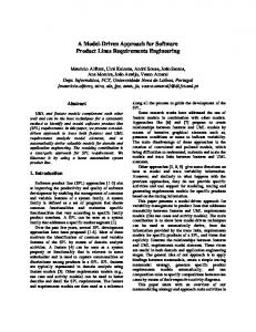
f Payment
...
fj
fk
fl Identity Federation
Payment Gateway Interface
Fraud Detection
Payment Method
fm
[5 , 17]
fn
Notification
23 Credit Card Credit Card Debit Card Payment Validation Payment EmailVoicemail
Phone Fax
Payment Process
fi
[17 , 48]
[8 , 20]
[12 , 30]
[10 , 45]
[15 , 51]
[8 , 27]
[3 , 35]
[10 , 54]
Mobile-based Notification
k k Or
Group Require & Exclude Cardinality Constraints Feature Model Notation
Alternative Optional Mandatory
Process Pool
Activity
Gateway
Sequence Flow
BPMN Notation- Basic constructs
(a)
(b)
Fig. 1. a) Feature model representing structural variability in business process family b) E-payment feature and its process flow.
2.1
Illustrative Example
In Fig.1, we show a simplified business process model for e-Payment in a global online retailer scenario to illustrate the concepts and further discussions. As shown, different features from the feature model (on the left) can be used within the business process model (on the right) to implement the functionality of the payment process. These features can be realized using appropriate services, which can have different QoS characteristics. For example, the activities represented in gray color in the process model indicate optional features; i.e., those features can be optionally included or excluded from the target product based on stakeholders’ requirements. For instance, the Notification feature can be included in a product by selecting one of the Mobile-based notification, Phone-Fax notification, or Email/Voicemail notification features, which have different range of quality values, since they are implemented by different services. Hence, the QoS characteristics of a developed product is closely dependent upon the features that get included in a final product. 3
A feature model such as the one in Fig.1(a) is a model of a family of products (SPL), which in turn represents a general customizable SaaS, while each variant (customized service) is a member of that family. Variation points are considered those places in the design of the SOSPL architecture where a specific decision has been narrowed down to several options. However, the options to be selected for a particular application w.r.t. stakeholders’ requirements are left open for configuration. Hence, variation points provide the possibility to derive different products, i.e., different final composite services. In SOSPL, particularly during the domain engineering cycle, determining the implied QoS ranges for individual features, based on the underlying architecture and implementation, helps domain engineers ensure that the product line architecture will fulfill and deliver the upper and lower bounds or values of quality requirements requested by stakeholders. In other words, the aggregation of the QoS properties of a feature model based on the QoS characteristics of its features, as derived from underlying processes and services implementing those features, provides the means to estimate the likely lower and upper bounds of QoS properties for potential products that will be derived from that product family. In addition, in the context of SOSPL, quality range computation through the construction of a generic evaluation model enables us to keep track of the product line quality ranges even during or after specifications of the service quality have changed. Therefore, the main contribution of this work is an introduction of the process how these QoS ranges are computed in the presence of variability. 2.2
Feature Modeling
As described above, a feature represents system functionality, which can be either a functional or quality feature. Hence, a feature is essentially a design-level concept depicting the functional capabilities of a domain. Feature modeling is one of the important techniques for capturing, modeling and describing the commonalities and differences between the products of a family based on their features. Moreover, feature modeling allows to abstract variability in stakeholders’ requirements, which in turn simplifies the process of customization of the family into individual products by automating analysis and reasoning on created feature models. It also prolongs to support customization framework in order to support dynamic deployment of variant business processes. A feature model is a means for describing a permissible configuration space of all the products of a family in terms of its features and their relationships. A feature model consists of both formal semantics and graphical representation, which is a rooted directed acyclic graph (DAG). Feature diagram, which is a tree-like graphical notation, is more widely used due to its visual appeal and easier understanding. In the tree-like structure, each node (feature) represents a variation or increment in application functionality. Fig.1(a) depicts a part of the feature model in our example, which describes common and variable features and represents architectural variability in the reference business process model. Parent-child relationships in the feature diagram indicate the refinement of application functionality. As not all features are assumed to be present in every product, this differentiation is expressed by a classification of feature types and relationships, which drive architectural variability patterns as follows: 1. Mandatory-Optional: A mandatory feature must be included in every member of a product line if its parent feature is selected. An optional feature may or may not be included if their parent is included; 4
2. Or groups: Or feature groups are non-empty subsets of features that can be included if a parent feature is included; 3. Alternative groups: Alternative feature groups indicate that from a set of alternative features exactly one feature must be included if the parent of that set is included. We formally define a feature model as follows: Definition 1 (Feature Model). A feature model FM = GFM (V, E) is a directed acyclic graph consisting of the set of vertices V representing features and edges E ⊆ V × V • ◦
representing the parent-child relations between the features, such that E={f , f , for , fxor }, •
◦
where f and f denote mandatory and optional parent-child feature relations, respectively; for and fxor denote Or and Alternative group relations between parent-child features with common parents, respectively. In general, cardinality is also defined among a group of n > 1 sub-features, which is denoted by < k − k 0 >, where 1 ≤ k ≤ k 0 ≤ n. Hence, < k − k 0 > cardinality defined over Or feature groups indicates at least k and at most k 0 features that can be included out of the n features in a group if the parent is selected. For example, in Fig.1(a), cardinality specified for the Notification feature indicates that all of the product members must at least have two notification features. Moreover, the cardinality specified for Alternative feature groups implies that only k out of n features in the group must be included if the parent is selected. In addition, integrity constraints, i.e., the includes and excludes relations, can be defined over features of a feature model. They are the means to express that the presence of a certain feature in the product imposes the presence or exclusion of another feature. As it can be observed, except for the mandatory feature type, all the other types of features imply architectural variability. Variation points are those features that have at least one direct variable sub-feature. 2.3
Reference Business Process Model
A template-based approach, where a reference model is designed as a template and is further customized for various purposes, has been widely adopted by practitioners [6]. The business process modeling community has also defined reference business process models. The reference model contains a union of the business processes for the entire product line in a superimposed way. The reference model provides the common business logic for orchestration and choreography of services. This reference model can be modeled using process-oriented modeling languages, e.g., BPMN, EPC, and/or YAWL. The design of reference models is accomplished in the course of the domain engineering lifecycle [5]. The configuration (tailoring and customization) of a reference models is performed by the selection/elimination of features from the feature model. In other words, due to the fact that architectural variations in the reference model are encoded as features, the various parts of the reference business processes are organized in variation points, which are managed and configured by means of feature models. Thereby, during the application engineering, the reference business process model can be configured to specific needs of different stakeholders based on the selected prioritized features. It should be noted that we distinguish between design and runtime variability. Feature models capture and encapsulate only architectural variability at design time. In contrast, business process models describe behavioral variability, i.e., how features are composed, which drives runtime variability through composition patterns (discussed in the next section). Furthermore, feature 5
model configuration is performed during the build-time. The configuration can be fulfilled through the process of staged-configuration where features are prioritized and selected according to the (non-)functional requirements of the stakeholders [7]. We consider a business process model as a workflow which is formally defined as follows: Definition 2 (Business Process Model). Business process model BP is defined as a directed acyclic graph GBP =(V, E), where V = {n� , Vσ , VA , VG} denotes a set of disjoint nodes, n� is a unique initial state,Vσ is a final state, VA is a set of activities, and E represents the edges (transitions) between the nodes. VG is a set of nodes as gateways. A business process is viewed as a series of activities where an activity represents a functional abstraction of services. An activity can be 1) atomic (a.k.a., task) or 2) nonatomic (a.k.a., sub-process). Each activity is delegated and bound to one or more services that provide the required functionality with different quality properties. Gateways, as routing constructs, represent a control flow of branchings, i.e., routing points. In this paper, we impose the following well-formedness conditions on a business process structure [8]: i) a business process model has a single source node, i.e., a node with no incoming edge; ii) every activity node has a single incoming and a single outgoing edge; iii) for every node with multiple outgoing arcs (i.e., a split), there is a corresponding node with multiple incoming arcs (a join), such that the set of nodes between the split and the join forms a single-entry-single-exit region [9]. In our work, architectural and behavioral variability are described by means of two models, i.e., feature models and business process models, respectively. Hence, we will assume that there is a mapping model available which interconnects these two models [3,6]. This injective mapping (i.e., one-to-one) reciprocally links each feature in the feature model to the corresponding activity in the reference business process model.
3
Quality of Service Aggregation and Computation for Product Line Architecture
In this section, we describe our proposed quality aggregation model for product line architectures. We will cover the following issues in order to provide a model for aggregating and computing QoS range values in the presence of variability: 1) quality criteria and quality range values for SOSPL; 2) the combination of variability and composition patterns; 3) based on the combination of variability and composition patterns; and 4) computational algorithms for computing aggregate quality range values. 3.1
Quality Criteria for Service-Oriented Product Line
There is very little agreement on a common vocabulary to describe non-functional properties (QoS). Because different domains and applications may require dissimilar sets of QoS properties; consequently, a wide range of heterogeneous quality models can be developed and do in fact exist. Different fields of research and standards have proposed diverse definitions and ontologies for describing QoS properties based on their target application domains [10]. Nevertheless, a widespread standard for the specification of quality properties such as performance, availability and security does not exist. We consider some quantitative QoS characteristics of Web services, which have been taken into consideration as selection criteria in the research literature [11,10,12,13]. Specifically, cost and response 6
time will be the two indexed QoS properties included in our work, which will be denoted by qpr and qrt , respectively,throughout the paper. Of course, our approach is not limited to these two QoS types, but these are the only discussed here due the limited space of the paper. Within the SOSPL architecture, the aggregation and evaluation of quality range values are performed based on the quality of services provided by the features in the product line. We assume that the QoS values are available through service profiles. In this work, we include the following indexed QoS properties: 1)cost, 2)response time, 3)throughput, 4)availability, which are denoted as qpr , qrt , qtr , and qav , respectively. Let us now proceed with some formal definitions as a basis for our work. Definition 3 (Quality Range). The quality range values of the ith quality property (dimension) is defined as qiR = [qiLB , qiUB ], where qiLB and qiUB are lower and upper bound values of the quality property, respectively. The above definition shows that each property such as response time or cost can be described by a range of numerical values. This range specifies both lower and upper bounds for that quality property. In order to be able to compute such a quality range, appropriate aggregation operators are needed. We consider the following three types of quality aggregation operators for computing the quality ranges of a software product line: • Summation: The quality range values of the product line is determined by a sum of the QoS ranges values of the quality attributes of services. An example would be cost; • Multiplication: The range values of quality attributes is determined by production of the QoS values of the services, for instance, reliability and availability; • Min-Max: The quality range values of the product line is computed with respect to critical paths [10,14] in the business process structure, for instance, response time (i.e., execution duration). In order to employ the above operators, we consider the following. We assume that for each activity an∈VA in a business process model BP , there is a bounded set of candidate services, San =hsn1 , . . . , snm i, in which all of the candidates provide the same functionality, but with different degrees of QoS properties. The quality of a service s is a vector Qs = hq1 (s), . . . , qk (s)i ∈ R, where the function qi (s) determines the values of the ith quality property. The quality of each activity an is defined as a matrix [Qan ]i×j ; 1 ≤ i ≤ k, 1 ≤ j ≤ m, where each row corresponds to a quality property qi , while each column corresponds to a service candidate. Thereby, the range of the ith quality property for feature fn corresponding to activity an is obtained by the quality range function qiR (fn ) = [qiLB , qiUB ], where UB qiLB = Qmin = Qmax an and qi an . For example, let us assume that there are five service candidates in Sa3 binding to activity a3 , mapped to feature f3 , and that their service cost values (qpr ) are given by vector Qa3 (i, j) = h100, 250, 65, 130, 95i. The cost range values of feature f3 could be set R as follows: qpr (f3 ) = [65, 250], because we are interested in the lower and upper bound values for the quality range. 3.2
Combining Variability and Composition Patterns
In essence, the aggregation model for quality computation in the context of SOSPL depends on: a) structural variability captured by a feature model, b) behavioral variability captured by a business process model, which describes the composition structure. 7
Composition patterns1 , which have their roots in workflow management systems[15], aim at building composition structures that are derived from the requirements in the process modeling phase. In other words, these patterns describe the behavior of features during execution time.Composition patterns are independent of particular composition languages or techniques. They represent the abstract control flow and execution sequence of features within the reference business process model for the whole family. van der Aalst et al. [15] have presented a collection of patterns for the different aspects of process-oriented application development, which describes the sequence and control flow dependencies between activities in a workflow. In our work, we employ these patterns to build the quality aggregation and computation model. Similar to [13], we consider composition patterns that address the behavioral structure of a composition. These patterns can be grouped into two main groups: a) sequential patterns and b) parallel patterns. These patterns are defined in terms of how the process flow proceeds in sequences and splits into branches for executing the activities and how they merge or converge. For our work, we consider the combination of parallel split, convergence and synchronization patterns. In a process, two basic sequential patterns are defined as sequence and and arbitrary cycle. 1. Sequence: A sequence pattern describes the structure where an activity in a process execute after the completion of another activity in the same process. The order of executions is not pertained to the quality aggregation model. 2. Arbitrary cycle: This pattern denotes that the execution of one or more activities is repeated for a given number of times in control flow. Parallel patterns are major patterns in any business process models. These patterns are determined in terms of how the process flow splits into branches for executing the activities and how they merge or converge. 3. Parallel split: A parallel split pattern represented by AND-split operation describes the behavioral structure where a single thread of control flow splits into multiple threads which can be executed concurrently in any order. 4. Multi-choice: This pattern represented by OR-split operation describes the structure where a number of branches can be selected and then executed based on process control data and business rules. 5. Exclusive/Deferred choice: An exclusive pattern represented by XOR-split operation describes the behavioral structure where only one of several branch is selected for execution based on decision or process control data. Following general parallel patterns represent how branches model the logic of the convergence of activities executing in a process flow. 6. Synchronization: This pattern represented by AND-join operation describes the structure of process where multiple activities in parallel branches converge into one single thread synchronized. 7. Simple-merge: The simple merge pattern represented by XOR-join operation describe the structure where multiple branches converge without synchronization and only one of alternative branches has been executed in parallel. 1
We use the terms workflow and composition patterns, interchangeably.
8
ICSOC paper
Sequential Patterns
f CP1: Sequence
...
f1
CP2: Loop Parallel Patterns
fn
f k k
f1
f2
...
CP3: Parallel split – Synchronization (AND-AND)
CP4: Parallel split – Discriminator (AND-DISC)
CP5: Parallel Split – Simple merg (AND-XOR)
CP6: Multi-Choice – Sync. merg (OR-OR)
CP7: Multi-choice – Discriminator (OR- DISC )
CP8: Multi-choice – Simple merg (OR-XOR)
fn
Or
f k k
f1
f2
...
fn
Activity: Task/Sub-process
fi
Mapping
⊆
Alternative
,
| ∈ ,
∈
}
Gateway
CP9: Exclusive – Simple merg (XOR-XOR)
Variability Patterns
AND OR XOR m/n
Composition Patterns
Fig. 2. Variability and composition patterns
8. Multi-merge: This patterns describe the structure where branches converge without synchronization and the activity succeeding the mergence will be activated by the completion of every incoming branch. This pattern can be modeled by AND-splits and AND-join operations. 9. Discriminator/m-out-of-n-join: In discriminator pattern, subsequent activity will be executed by the first and only the first branch completed based on the condition and all the rest of branches are disregarded. The discriminator patterns can be generalized where the subsequent activity will be activated only after m-out-of-n activity. It should be noted that various combinations of parallel split and join cannot semantically and formally provide valid patterns. For example, XOR-split in combination with ANDjoint cannot occurs in process, hence it does not generate valid pattern. Fig.2 illustrates three variability patterns (left side), as described in Sec.2.2, in combination with nine composition patterns (CP1-CP9) represented using BPMN notation (right side). We perform quality aggregation based on a set of proposed aggregation rules described below.
3.3
Aggregation Rules based on Variability and Composition Patterns
Based on the patterns described above, we define aggregation rules for each QoS property by primarily taking into account the variability patterns which may occur within each composition pattern. In the following, we present the aggregation rules for two numerical QoS properties: cost and response time (i.e., execution time). The cost of a feature is the cost which can be associated with the deployment, execution, management, maintenance and monitoring of a service. The aggregation rules for availability and throughput are presented 9
in a longer version of the current paper which is accessible online2 . The summary of the aggregation rules that we have defined are given in Tables 1 and 2. Table 1
Table 1. Aggregation rules based on Mandatory-Optional variability patterns Cost (qc)
Seq. Patterns
• n LB q pr ( f i ) : ∀f i ∈ f i =1
I. Sequence II.
• n LB q pr ( f i ) : ∀fi ∈ f i =1
IV. AND-DISC
VI. XOR-XOR VII. OR-XOR VIII. OR-OR IX. OR-DISC
Seq. Patterns
pr
i =1
• ( f i ) : ∀f i ∈ f ∨ f
• n LB q pr ( f i ) : ∀f i ∈ f i =1 • LB cqrt ( f i ) : f i ∈ f ∨ f
•
cq pr ( f i ) : f i ∈ f ∨ f
,
UB
q pr ( fi ) : ∀fi ∈ f ∨ f i =1 n
,
• LB min q pr ( f i ) : f i ∈ f ∨ f
•
UB
,
n
• ( f i ) : ∀f i ∈ f ∨ f • UB cqrt ( f i ) : f i ∈ f ∨ f
, q
UB pr
i =1
,
• LB max qrt ( f i ) : ∀f i ∈ f i
,
max qrt ( f i ) : ∀f i ∈ f ∨ f
LB min qrt ( f i ) : ∀f i ∈ f i
,
max qrt ( f i ) : ∀f i ∈ f ∨ f
•
• UB max q pr ( f i ) : f i ∈ f ∨ f
,
LB min q pr ( f i ) : ∀FSub ∈ F n Cm f ∈F i Sub
• LB min qrt ( f i ) : ∀f i ∈ f ∨ f
•
UB
•
UB
,
• UB max qrt ( f i ) : ∀f i ∈ f ∨ f
UB 1 max q pr ( f i ) : ∀FSub ∈ F n Cm min max q LB ( f ) : f ∈ F , ∀F ∈ F f ∈F n pr i i Sub Sub i Sub Cm
,
• UB max qrt ( f i ) : ∀fi ∈ f ∨ f
rd
For example, assuming three features (m =3) out of seven (n=7) in CP6-CP7, the minimum of 3 quickest should be considered Availability (qav)
QoS Properties I. Sequence II.
• n LB ∏ qav ( f i ) : ∀f i ∈ f ∨ f i =1 • C LB qav ( f i ) : ∀ f i ∈ f ∨ f
Arbitrary Cycle
III. AND-AND IV. AND-DISC Parallel Patterns
Response Time (qrt) UB
V. AND-XOR
1
Mandatory-Optional Variability Pattern
n
, q
• LB cq pr ( f i ) : f i ∈ f ∨ f
Arbitrary Cycle
III. AND-AND
Parallel Patterns
Mandatory-Optional Variability Pattern
QoS Properties
V. AND-XOR VI. XOR-XOR VII. OR-XOR VIII. OR-OR IX. OR-DISC
• n LB ∏ q av ( f i ) : ∀ f i ∈ f i =1
i
• ( f i ) : ∀f i ∈ f
• UB C qav ( f i ) : ∀ f i ∈ f ∨ f
n
, ∏q
LB min ∏ qav ( fi ) : ∀FSub ∈ F n Cm f ∈F Sub
UB av
i =1
,
• LB min qav ( fi ) : ∀fi ∈ f ∨ f
Throughput (qtp)
n
, ∏q
UB av
i =1
( fi ) : ∀fi ∈ f ∨ f •
,
max qav ( f i ) : ∀fi ∈ f ∨ f
,
UB max ∏ qav ( f i ) : ∀FSub ∈ F n Cm f ∈F Sub
UB
•
i
• LB min qtp ( f i ) : ∀f i ∈ f ∨ f
,
• LB qtp ( f i ) : f i ∈ f i ∨ f i
,
qtp ( f i ) : f i ∈ f i ∨ f i
• LB min qtp ( f i ) : ∀f i ∈ f ∨ f
,
• UB min q pr ( f i ) : ∀f i ∈ f ∨ f
• LB min qtp ( f i ) : ∀f i ∈ f ∨ f
,
max qtp ( f i ) : ∀f i ∈ f ∨ f
• LB min qtp ( fi ) : ∀fi ∈ f ∨ f
,
• UB max q pr ( f i ) : ∀f i ∈ f ∨ f
•
UB
UB
•
max min qtp ( fi ) : fi ∈ FSub , ∀FSub ∈ F UB
Cm n
According to Definition 3, the definition of a lower bound, qiLB , for different quality properties must indispensably consider the mandatory features for sequential and parallel split patterns (CP1-CP4). In addition to mandatory features, the optional features generally contribute to the upper bound range value, qiUB . For instance, in the sequential patterns, the cost of feature f should be determined by the sum of the cost values of each mandatory features for the lower bound; while the upper bound is determined by the accumulated cost for mandatory as well as optional features. By adopting a hierarchical approach, described in the next section, the range values (upper and lower bounds) for QoS properties are computed for a combination of variability and composition patterns, based on our formulated aggregation rules. To determine the upper and lower bounds for QoS range values, qiR (f ), for a parent feature f (see Fig.2), the aggregation rules are applied on the basis of each composition pattern according to the variability patterns. To further introduce the principles of our aggregation model, the following explanation is provided. Feature set FCln contains all of the permissible combinations of the feature sets, where the number of distinct l-element subsets is a binomial coefficient denoted as Cln . To compute the quality range values, the aggregation operators are applied to each member set of FSub∈FCln . For instance, for the lower and upper range values of cost (qpr ), 2
http://qos-sospl.sourceforge.net/
10
Table2
Table 2. Aggregation rules based on Or and Alternative variability patterns
Seq. Pattern Parallel Patterns
Or(*)1 / Alternative(**)1 Variability Patterns
QoS Properties 1
Sequence
3
AND-AND
4 5 6 7 8 9
Seq. Pattern Parallel Patterns
Response Time (qrt)
LB min q pr ( fi ) : ∀FSub ∈ F n f ∈F C k i Sub , (*) (**) AND-DISC UB AND-XOR max q pr ( fi ) : ∀FSub ∈ F n | F n Ck ′ Ck OR-XOR fi∈FSub OR-OR OR-DISC XOR-XOR
QoS Properties
Or(*) / Alternative(**) Variability Patterns
Cost (qc)
1
Sequence
3
AND-AND
4
AND-DISC
5 6 7 8 9
AND-XOR OR-XOR OR-OR OR-DISC XOR-XOR
Availability (qav)
LB min qrt ( fi ) : ∀FSub ∈ F n f ∈F Ck i Sub
,
(*) (**) UB max qrt ( fi ) : ∀FSub ∈ F n | F n f ∈F C Ck ′ k i Sub
LB min max qrt ( fi ) : ∀FSub ∈ F Ckn
,
(*) (**) UB max max qrt ( fi ) : ∀FSub ∈ F n | F n Ck ′ Ck
LB min min qrt ( fi ) : ∀FSub ∈ F Ckn
,
(*) (**) UB max max qrt ( fi ) : ∀FSub ∈ F n | F n Ck ′ Ck
LB min max qrt ( fi ) : ∀FSub ∈ F Ckn
,
(*) (**) UB max max qrt ( fi ) : ∀FSub ∈ F n | F n Ck ′ Ck
Throughput (qtp) LB min min qtp ( fi ) : ∀FSub ∈ F Ckn
LB min ∏ qav ( fi ) : ∀FSub ∈ F n f ∈F C k i Sub min min qtpLB ( fi ) : ∀FSub ∈ F , Ckn (*) (**) LB max ∏ qav ( fi ) : ∀FSub ∈ F n | F n f ∈F Ck ′ Ck i Sub LB min min qtp ( fi ) : ∀FSub ∈ F Ckn
,
(*) (**) UB max max qtp ( fi ) : ∀FSub ∈ F n | F n Ck ′ Ck
,
(*) (**) UB min min qtp ( fi ) : ∀FSub ∈ F n | F n Ck ′ Ck
,
(*) (**) UB max max qtp ( fi ) : ∀FSub ∈ F n | F n Ck ′ Ck
1
(*) and (**) represent the feature set combinatorial operators which are applied for Or and Alternative variability patterns, respectively
the summation operator is first applied to each element of FSub , which results in a new set. For this new set, the min-max operator is then applied. The mandatory and optional features in the Multi-choice parallel patterns (cf. CP6, CP7 and CP8) follow different aggregation rules. To determine the lower and upper bounds, the aggregation model also requires knowing which paths in the business process flow will be chosen at runtime particularly for OR-Splits. We assume that an execution of all possible choices for an OR-Split gateway is equally probable. The business rules defined over business process models (i.e., OR-Split gateway) specify how many paths (m) can be 0 n where k ≤ m ≤ k ≤ n. executed at runtime. This results in a feature set FSub ∈ FCm For instance, in our example, assume that two notification features Email-voicemail and Mobile-based notification are included in an instance of the reference business process. Hence, the decision concerning which notification service should be invoked w.r.t. OR-split semantics is left to runtime. To address Or group and Alternative group feature variability in combination with Multi and Exclusive choice composition patterns (CP7, CP8, and CP9), the aggregation model must consider all possible combinations of features corresponding to the given cardinality over the n features of the feature group specified at design time. Therefore, the resulting feature set (i.e., FSub ) is a subset of FC k0 and FCkn0 for lower and upper bound k quality range values, respectively.
3.4
Quality of Service Range Aggregation
The QoS range values for features in a feature model are computed by hierarchically aggregating the QoS for variability patterns at the level of each composition pattern. Aggregation 11
C1
C10 C9
VG5 VG1 C2
C4
C1
VG6
C12
C8
C6
VG3
C13
C5
C14
(a)
C2
C3
f1
f2
C4
C5 C7 VG2 VG3 C12 C13 C14 VG4
VG2 C6
f4
VG2 C7
C3
C11
VG4
f9 f10 f11
VG5 C9 C8 VG6
f7 C10 C11 f6
f8
(b)
Fig. 3. a) Decomposition of business process model to SESE components. b) Business process structure tree.
is performed by gradually collapsing features into a single feature in the feature model, by employing the notion of a virtual feature. This approach enables us to perform the aggregation from both micro and macro perspectives. In other words, the quality range values can be computed for each of the given features from a local view and also for the entire feature model from a global view. Algorithm 1: Aggregate QoS range for feature: AggregateQoSRange(f ) Input: f : given feature of feature model FM Output: QoS reange- q R of f eaturef 1 begin // All direct child features of f ; 2 Sf [ ] ←− ∀ChildF eatureOf (f ) ; 3 if Sf = ∅ then return q R (f ); 4 else 5 for i = 1 to |Sf | do 6 AggregateQoSRange(Sf [i]); 7 P ST ←− ProcessStructure(Sf [i]); 8 if P ST = ∅ then return q R (f ) else q R (f )= ComputeQoSR(P ST ) 9 10
end
Algorithms 1 and 2 detail the procedure for computing QoS ranges for a feature model. In these algorithms, the feature model is traversed from a given feature node by post-order depth-first traversal, i.e., computing the aggregated QoS ranges from leaves and the right-most nodes up to the root node. For each feature, the business Process Structure Tree (PST) corresponding to a given feature is subsequently created and parsed (Fig.3(b)). For every trivial Single-Entry Single-Exit (SESE) component in PST, the control flow analysis is performed, whose details are omitted from Alg. 2 for the sake of brevity; interested readers are referred to [16]. In order to analyze and identify how features at the same level in the feature model are composed, we decompose the process graph into process components (Fig. 3). A process component is a subgraph of the composition model with a SESE region, which may include individual tasks but also larger subgraphs. We employ the Refined Process Structure Tree (RPST)-based approach proposed in [14,9] to create and parse the process model into a tree of SESE components (line 7 in Alg. 1). 12
Alg. 2 operates over a PST, and the aggregation is performed at the level of each processes component. Lines 3 to 18 iteratively aggregate the quality for each child component. For individual process components, features are grouped into virtual features corresponding to the variability patterns. Algorithm 2: Compute QoS range values of business process associated to feature f : ComputeQoSR(C) Input: C : Process component- node of process structure tree P ST Output: q R : aggregated QoS range of process component 1 begin 2 foreach Ci ∈ ChildOf (C) do ComputeQoSR(Ci ) 3 forall fk ∈ Ci do // [1]Group features w.r.t. variability patterns and step-wise collapsing features by means of virtual features; 4
switch feature fk .Type do ◦
5 6 7
•
case fk ∈f ∨ f fVmo [ ] ←− fk ; q R (fVmo ) = AggQoS(fVmo ) w.r.t. Formulas in Table 1; ◦
8 9
◦
•
if ∀fk ∈ fVmo : fk ∈f then fVmo .Type=f else fVmo .Type=f ; case fk ∈ an Or-group •
fVor [ ] ←− fk ;
10
•
11 12
•
q R (fVor ) = AggQoS(fVor ) w.r.t. Formulas in Table 2; case fk ∈ an Alternative-group •
13
fVxor [ ] ←− fk ;
14
q R (fVxor ) = AggQoS(fVxor ) w.r.t. Formulas in Table 2;
•
•
15
end
16
fV [ ] ←− fVmo , fVor , fVxor ; q R (fV ) = AggQoS(fV ) w.r.t. Formulas given in Tables 1,2;
•
• 17
• 18 19 20 21
•
◦
if ∃fk ∈ fV : fi ∈f then fV .Type=f else fV .Type=f ; end return q R (fV ) end
The control flow information is used for identifying the pattern in each of the SESE components. The virtual features, which are denoted as fVmo , fVor , fVxor , represent Mandatory-Optional, Or and Alternative grouped virtual features, respectively. Quality range values of virtual features are computed by an aggregation function (AggQoS) according to the aggregation rules introduced earlier in the paper and shown in Tables 1 and 2. In order to comply further with the aggregation rules,, the type of virtual features should also be determined. Hence, the type of the corresponding virtual feature is labeled as optional if all the collapsed features are optional, otherwise it is labeled as mandatory (i.e., Line 8). However, it is noted that according to the given semantic descriptions of feature variability of Or and Alternative groups, corresponding virtual features fVor and fVxor are labeled mandatory. The virtual feature fV includes all of the collapsed virtual features, which are grouped in each basic composition patterns, and its type is determined such that 13
f
f
1
f
2 2
f1
f2
f3
[8,20]
[17,48]
f5
f4
f1
[10,54]
23
f2
f3
f5
f4
[8,20] [17,48]
[10,54]
f1
f2
[8,20]
23
f6,8,7
f5
f4
[17,48] [12,51]
[10,54]
23
1
f6
f7
f8
f9
f10
f11
f6,8
f
f9
f7
f
3
f2
f11
f9
f4,6,8,7
[8,20] [17,48] [12,105]
f9
f1
f5 23
f10
f2
f
4
f4,6,8,7
[8,20] [17,48] [12,105]
f10
f11
[10,45] [8,27] [3,25]
5
4
3
f1
f10
[12,47] [15,51] [10,45] [8,27] [3,25]
[5,17] [15,51] [12,30] [10,45] [8,27] [3,25]
6
f
5
f9,10,11
f1
f2,4,6,8,7,9,10,11
[11,97]
[8,20]
[40,250]
[40,270]
f11
[10,45] [8,27] [3,25]
Fig. 4. Step-wise feature model transformation
if there is at least one mandatory feature in a grouped feature, the type of the collapsed virtual features is considered mandatory as well (line 18). To exemplify the aggregation algorithm described above, we compute the QoS range values for the payment feature in the feature model shown in Fig.1. Furthermore, Fig.4 depicts the step-wise transformation of the feature model through gradual hierarchical aggregations. The following is also the step-wise process for computing the QoS range values for the payment feature. To show how each of the transformations is actually performed and how the range values are computed, we refer to the relevant lines of the algorithm that is used besides each step.
R qpr (f ) =
�
LB UB R [qpr , qpr ] := qpr (fV )|fV = Agg.
◦
•
◦
n S
� fi
(Alg.1 lines 2-11)
i=1
R R R (f 4 ) = [10, 54]; (Alg.1 lines 3) (f 2 ) = [17, qpr (f 1 ) = [8, 20]; qpr � 48]; qprX � • • • ◦ �R ◦ � UB • R LB UB R qpr (fV1) = qpr (f 6 ), qpr (f8 ) = qpr (f 8 ) , (Alg.2 lines 5-8) qpr (f 8 ), qpr (f 6 ) = [12, 47]; | {z } {z } | 1 1 Table1-Agg.rule No.1 � � � � �� • • • • ◦ � � LB • � UB • R R LB UB R qpr (f 3 ) = qpr (fV1), qpr (f7 ) = min qpr (fV1), qpr (f7 ) ,max qpr (fV1), qpr (f7 ) (Alg.2 lines 5-8) | {z } | {z } 2 1
Table1-Agg.rule No.6
= [12, 51]; � � X� • ◦ • • ◦ �R • R LB UB UB R (f 3 ) , qpr (f 3 ), qpr (f 4 ) = [12, 105]; qpr (fV2) = qpr (f 3 ), qpr (f 4 ) = qpr | {z } | {z } 3 1
Table 1.Agg. rule No. 3
14
(Alg.2 lines 5-8)
•
�
R qpr (f 5 ) = min
� X
LB qpr (fi ) : ∀FSub ∈ FC 3 2
�
� X �� UB , max qpr (fi ) : ∀FSub ∈ FC 3 3
fi∈FSub
(Alg.2 lines 9-11)
fi∈FSub
{z
|
}
4
1 Table 2.Agg. � � rule No.7 � �� � � � � � P� P = min {f9 ,f10}, {f9 ,f11}, {f10 ,f11} ,max {f9 ,f10 ,f11} = min 18, 13, 11} ,97 = [11, 97];
�
• ◦ • �R • R R R (Alg.2 lines 5-8) qpr (fV3) = qpr (f 2 ), qpr (f 5 ), qpr (fV2) | {z } 5 1 � �X • ◦ • • X� � LB • UB UB UB LB qpr (f2 ), qpr (f5 ), qpr (fV2) = [40, 250]; = qpr (f2 ), qpr (fV2) , | {z } No. 1 �Table 1.Agg. rule � X� • ◦ • • • �R ◦ UB UB LB UB R R qpr (f2 ), qpr (f5 ), qpr (fV2) = [40, 270] qpr (f ) = qpr (f1 ), qpr (fV3 ), (fV3) = qpr {z } | | {z } 6 1
4
Table 1.Agg. rule No.1
Discussion
In this section, we analyze the computational complexity of the proposed aggregation method, and then critically discuss its advantages and disadvantages. 4.1
Complexity Evaluation
The proposed QoS aggregation model includes the following three high-level steps: 1) quality range aggregation of features for feature models; 2) process structure tree construction related to each feature and finding canonical process components based on composition patterns; and 3) aggregation of QoS of process components w.r.t. aggregation rules and their propagation over the feature model. The size of the state-space in a feature model depends primarily on the size of the given feature model graph GFM(V, E). Backtracking of a feature model produces an ordering of the features in which the parent nodes are placed in post-order of their ancestors. The traversal of a feature model requires O(|VFM|+|EFM|), which has linear time complexity. Given the presence of integrity constraints (includes and excludes relations) in a feature model, the size of the resulting graph will be proportional to the number of constraints. This step could have exponential time complexity if the number of integrity constraints on a feature model is too high. We show below that this is usually not the case. In the second step, the modular decomposition of business processes and the construction of PST is performed in linear-time proportional to the size of the directed graph of the business process (see [17]). The third step of the algorithm for computing and aggregating quality range values is achieved by parsing the PST of the business process model GBP(V, E) and control flow analysis via alternative post-order depth-first traversals. This step requires O((|VBP|+|EBP|).(C+S)), where C and S denote the execution time of control flow analysis for each process component; and computing quality range values according to both the aggregation rules and the size of candidate service lists for each activity. The time required for grouping features based on variability patterns and capturing quality values does not add any computational complexity and can hence be ignored. As a result, given that the worst-case time complexity of the first step can be in some cases exponential, the time complexity of the entire algorithm can be exponential in the worst-case. However, it is important to note that the algorithm has a linear time complexity 15
when the number of integrity constraints is smaller than the number of features in a feature model, which is usually the case based on our analysis of standard feature models available at http://www.splot-research.org/, where the number of integrity constraints to the number of features ratio is approximately 0.18. 4.2
Critical Analysis
As mentioned earlier, we have made some assumptions regarding the topology of the business process graph, i.e., the proposed aggregation method is performed over wellstructured business process models. Well-structured business processes have a number of desirable properties, which result in less sophisticated verification mechanisms [8]. However, such an assumption requires the transformation of any ad hoc business process graph into a structural business process model. Substantial amount of work for the transformation of unstructured and arbitrary business process models to structured models already exists [14,18,9,8]. Therefore, our proposed approach can be further adapted and applied to both structured and unstructured business process models (through transformation). The limitation of the presented aggregation model is that it has not considered the integrity constraints and dependencies between features to deliver a more precise aggregation of QoS values. This is left for future work. Revisiting our original formulated challenge, the goal of QoS range aggregation is to ensure that the required quality levels are achieved for SOSPL architecture for each product in the family. The proposed quality aggregation model considers variability patterns from both structural and behavioral perspectives. The presented approach is a step towards achieving quality-aware product line configuration. Even in this early stage of the development, this approach supports quality aware staged configuration. It can be used to assure that every stage yields a subset of products whose quality ranges satisfy the desired QoS ranges. Finally, this work can be further considered for facilitating the management and customization of multi-tenant cloud applications [19]. 4.3
Implementation Aspects
The prototype of our proposed approach has been developed through extending a chain of tools in Java as a set of Eclipse plug-ins. Cardinality-based feature-model is employed by FeatureMapper3 to model feature variability and perform SPL configuration. FeatureMapper also allows the mapping of features from the feature model to their realization in a business process, i.e., activity constructs, by means of an Ecore-based language.4 The Eclipse rBPMN Modeler5 is developed for modeling service-based business process. We employ these tools along with our implementation of the algorithms for computing QoS range values in the presence of variability.
5
Related Work
There are several contributions and previous studies addressing QoS aggregation in terms of different process model structures for composite services. The works of Cardoso et al. [12] and Jaeger et al. [13] are the seminal works in the literature, which address the aggregation and estimation of QoS values for Web services composition in well-structured 3 4 5
http://featuremapper.org/update/ http://www.eclipse.org/modeling/emf/ http://code.google.com/p/rbpmneditor/
16
process models based on (some) workflow patterns in the work by van der Aalst et al. [15]. In [12], the authors propose Stochastic Workflow Reduction (SWR) to compute and estimate the entire workflow QoS values. The SWR algorithm iteratively applies a set of reduction rules for some sequential and parallel patterns over a given structured process graph. Their proposed algorithm for aggregation makes it possible to predict the QoS performance of the entire process by repeatedly performing substitution until the whole process is transformed into one composite service node. In [13], where the aggregation method is the most similar to ours, a QoS aggregation method is proposed for composite Web services by considering workflow patterns and computing upper and lower bounds for QoS values. Authors represent a process model as a graph which is collapsed step-by-step by applying composition patterns. Hwang et al. [20] have proposed a probability-based method where a composite service is represented by a process structure, which is recursively parsed and analyzed to aggregate quality attributes. Mukherjee et al. [21] focus on addressing the QoS computation in BPEL processes by performing aggregation on an activity graph. In a more recent work [14], an aggregation approach employs RPST and supports process models which include unstructured components. Most of the above studies are related to our proposal. However, existing solutions do not consider the constituent structural variability of process models and do not address modeling and managing variation points, which may occur within such an architecture and can significantly impact the proper QoS aggregation. To the best of our knowledge, this is the first work that takes both structural and behavioral variability into account for evaluating QoS dimensions in the context of SOSPL.
6
Conclusion
In this paper, we have provided a systematic approach for QoS range aggregation to support evaluation of quality ranges captured by SOSPL(s), which further helps us for qualityaware product derivation. As the main contribution, we have identified a set of variability patterns which may occur within composition patterns and proposed new aggregation rules for QoS range computation. Furthermore, we presented an algorithm that analyzes variability and process models to aggregates QoS ranges for an SOSPL. The present work is a continuation of our previous works [3,4], where we have presented approaches for configuration of SOSPLs in the application engineering lifecyle. In those works, we also proposed a method for features prioritization based on stakeholders’ objectives and preferences concerning functional and QoS requirements. We also presented how that method can be leveraged by using linear optimization methods for optimal service selection within boundaries of constraints specified by the stakeholders. The approach presented in this paper takes our previous work to next stage where automatic computation of quality ranges in the presence of variability is made possible. As the future work, we also intend to evaluate how our proposed approaches for configuration enabled by the contribution of this work can be applied to real-world scenarios.
References 1. Cohen, S.G., Krut, R.: Managing variation in services in a software product line context. Technical Report SEI-2010-TN-007, Carnegie Mellon University (2010) 2. Lee, J., Kotonya, G.: Combining service-orientation with product line engineering. IEEE Software 27 (2010) 35–41
17
3. Mohabbati, B., Hatala, M., Gaˇsevi´c, D., Asadi, M., Boˇskovi´c, M.: Development and configuration of service-oriented systems families. In: Proceedings of the 2011 ACM Symposium on Applied Computing. SAC ’11, New York, NY, USA, ACM (2011) 1606–1613 4. Bagheri, E., Asadi, M., Gasevic, D., Soltani, S.: Stratified analytic hierarchy process: Prioritization and selection of software features. In: Software Product Lines: Going Beyond - 14th International Conference, SPLC 2010. Volume 6287 of LNCS., Springer (2010) 300–315 5. Pohl, K., B¨ockle, G., van der Linden, F.J.: Software Product Line Engineering: Foundations, Principles and Techniques. Springer-Verlag New York, Inc. (2005) 6. Czarnecki, K.: Mapping features to models: A template approach based on superimposed variants. In: GPCE 2005 - Generative Programming and Component Enginering. 4th International Conference, Springer (2005) 422–437 7. Czarnecki, K., Helsen, S., Eisenecker, U.W.: Staged configuration through specialization and multilevel configuration of feature models. Software Process: Improvement and Practice 10 (2005) 143–169 8. Kiepuszewski, B., Hofstede, A.H.M.t., Bussler, C.: On structured workflow modelling. In: Proceedings of the 12th International Conference on Advanced Information Systems Engineering. CAiSE ’00. Springer-Verlag, London, UK (2000) 431–445 9. Vanhatalo, J., V¨olzer, H., Koehler, J.: The refined process structure tree. Data Knowl. Eng. 68 (2009) 793–818 10. Zeng, L., Benatallah, B., Ngu, A., Dumas, M., Kalagnanam, J., Chang, H.: QoS-aware middleware for web services composition. Software Engineering, IEEE Transactions on 30 (2004) 311–327 11. Yu, T., jay Lin, K.: Service selection algorithms for composing complex services with multiple qos constraints. In: ICSOC. (2005) 130–143 12. Cardoso, J., Sheth, A.P., Miller, J.A., Arnold, J., Kochut, K.: Quality of service for workflows and web service processes. J. Web Sem. 1 (2004) 281–308 13. Jaeger, M.C., Rojec-Goldmann, G., Muhl, G.: Qos aggregation for web service composition using workflow patterns. In: Proceedings of the Enterprise Distributed Object Computing Conference, Eighth IEEE International, Washington, DC, USA, IEEE Computer Society (2004) 149– 159 14. Dumas, M., Garc´ıa-Ba˜nuelos, L., Polyvyanyy, A., Yang, Y., Zhang, L.: Aggregate quality of service computation for composite services. In: ICSOC. (2010) 213–227 15. Van Der Aalst, W.M.P., Ter Hofstede, A.H.M., Kiepuszewski, B., Barros, A.P.: Workflow patterns. Distrib. Parallel Databases 14 (2003) 5–51 16. Vanhatalo, J., V¨olzer, H., Leymann, F.: Faster and more focused control-flow analysis for business process models through sese decomposition. In: Proceedings of the 5th international conference on Service-Oriented Computing. ICSOC ’07, Berlin, Heidelberg, Springer-Verlag (2007) 43–55 17. McConnell, R.M., de Montgolfier, F.: Linear-time modular decomposition of directed graphs. Discrete Appl. Math. 145 (2005) 198–209 18. Ouyang, C., Dumas, M., Aalst, W.M.P.V.D., Hofstede, A.H.M.T., Mendling, J.: From business process models to process-oriented software systems. ACM Trans. Softw. Eng. Methodol. 19 (2009) 2:1–2:37 19. van der Aalst, W.M.P.: Configurable services in the cloud: Supporting variability while enabling cross-organizational process mining. In: On the Move to Meaningful Internet Systems: OTM 2010. Volume 6426 of LNCS., Springer (2010) 8–25 20. Hwang, S.Y., Wang, H., Tang, J., Srivastava, J.: A probabilistic approach to modeling and estimating the qos of web-services-based workflows. Inf. Sci. 177 (2007) 5484–5503 21. Mukherjee, D., Jalote, P., Gowri Nanda, M.: Determining qos of ws-bpel compositions. In: Proceedings of the 6th International Conference on Service-Oriented Computing. ICSOC ’08, Berlin, Heidelberg, Springer-Verlag (2008) 378–393
18