MeiÃner et al / VIZARD II: A Reconfigurable Interactive Volume Rendering System datasets and classifications where the volume can be en- coded efficiently ...
Graphics Hardware (2002), pp. 1–11 Thomas Ertl, Wolfgang Heidrich, and Michael Doggett (Editors)
VIZARD II: A Reconfigurable Interactive Volume Rendering System M. Meißner, U. Kanus, G. Wetekam, J. Hirche, A. Ehlert, W. Straßer† M. Doggett‡ , P. Forthmann, R. Proksa§ WSI/GRIS, University of Tübingen, Germany Philips Research Hamburg, Germany
Abstract This paper presents a reconfigurable, hardware accelerated, volume rendering system for high quality perspective ray casting. The volume rendering accelerator performs ray casting by calculating the path of the ray through the volume using a programmable Xilinx Virtex FPGA which provides fast design changes and low cost development. Volume datasets are stored on the card in low profile DIMMs with standard connectors allowing both, large datasets up to 1 GByte with 32 bit per voxel, and easy upgrades to larger memory capacities. Per-sample Phong shading and post-classification is performed in hardware, giving immediate feedback to changes in the visualization of a dataset. Adding new features, such as pre-integrated classification, can be accomplished using the existing card without expensive and time consuming redesigns. The card can also be used for medical image reconstruction by reconfiguring the FPGA broadening its usefulness for end users. For the first time, users are able to generate high quality perspective images as required for applications such as virtual endoscopy and colonoscopy, and stereoscopic image generation. Categories and Subject Descriptors (according to ACM CCS): I.3.1 [Computer Graphics]: Hardware ArchitectureGraphics processor; I.3.7 [Computer Graphics]: Three-Dimensional Graphics and RealismRaytracing; C.3 [Computer Systems Organization]: Special-Purpose and Application-Based Systems;
1. INTRODUCTION Visualization of volumetric datasets is driven by the need to reach a better understanding and insight of measured or computed data. Many scientific and increasingly everyday applications require this insight, including areas in medicine, geophysics, scientific simulations and industry. The user gains greater insight and understanding with higher accuracy, perspective images, and direct control over the image synthesis process. Two dimensional images can be generated from three di-
† {meissner, hirche, wetekam, kanus, ehlert, strasser}@gris.unituebingen.de, WSI/GRIS, University of Tübingen, Sand 14, D72076 Tübingen Germany, phone: +49 7071 29 76361, fax : +49 7071 29 5466, ‡ ATI, USA § Philips Research Laboratories, Hamburg Germany c The Eurographics Association 2002. °
mensional volume datasets using either indirect or direct volume rendering. Indirect volume rendering involves transforming the dataset into another representation, such as triangles in the case of the Marching Cubes algorithm 11 . A triangle representation can then be easily rendered in realtime using modern 3D graphics hardware, but only specified iso-values are represented and a change in these values results in a non-interactive pre-processing stage. Furthermore, semi-transparent iso-surfaces are a hard problem at interactive frame-rates since they require depth sorting of all triangles prior to rendering. Direct volume rendering involves generating final pixel values by compositing together filtered samples of the original voxel values. In order to achieve interactive frame-rates this approach can be implemented in software, using readily available graphics hardware, or special purpose hardware. Shear-Warp 8 is recognized as the fastest software renderer to date and uses an image and volume encoding. For
Meißner et al / VIZARD II: A Reconfigurable Interactive Volume Rendering System
datasets and classifications where the volume can be encoded efficiently, interactive frame-rates can be achieved. However, interpolation is only bilinear, the encoding scheme requires significant pre-processing time—making interactive changes to the classification cumbersome—, and for semitransparent rendering, the overall performance drops significantly.
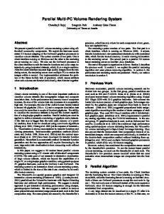
a combination of slab based orthographic projections 21 but the images are not free of artifacts and the performance is significantly reduced. In this paper, we describe a novel interactive volume rendering system based on a unique hardware accelerator. The system is realized as a custom designed PCB with off-theshelf components, as shown in Figure 1. Images are gen-
2D and 3D texture mapping hardware can also be used for volume rendering using a variety of techniques. By resampling a 3D texture map using texture mapped planes parallel to the view plane 2 , interactive frame-rates can be achieved on the SGI Reality Engine 1 . Texture mapping illumination limitations can be overcome by storing gradients for iso-surfaces allowing for illumination calculations to be performed 22 . While several people extended 14 and improved this approach 18 , it is generally inaccurate because the shading is based on the dot product of a nonnormalized interpolated gradient vector. Texture mapping has also been extended to support shading of iso-surfaces using pre-integration 4 and multi-dimensional transfer functions 6 . Despite the excellent results, these techniques either require multi-pass or a high sampling frequency, significantly reducing the frame-rate. Several approaches using custom hardware have also been proposed and implemented and a more general survey can be found in 17 : Knittel 7 presented a true ray casting architecture—named VIZARD—capable of providing a few frames per second for 2563 datasets. The PCI based accelerator uses the host main memory to store the volume data and utilizes FPGAs. Before rendering, the data is pre-shaded and compressed in software using a lossy compression scheme. The system is limited by the inability to change classification and shading. This is due to the pre-processing stage and the use of main memory to store the volume dataset, resulting in the performance being severely restricted by the PCI bus. The VIZARD II architecture proposal, presented in 15 , introduces a volume rendering pipeline with on-board memory and on-the-fly classification and shading. However, the architecture relies on discretized compressed gradients and its memory interface limits the overall frame-rate. VolumePro 16 delivers insight and control over the rendering process of a volume dataset unlike any previously available solution to real-time volume rendering. VolumePro’s performance is due to its architecture and the use of ASIC technology, providing unprecedented frame-rates. The scalable parallel pipelines in the VolumePro architecture relies on the availability of neighboring voxels in the pipeline which means that the generation of perspective images as well as the use of arbitrary sampling distances is not feasible or requires multi-pass approaches. Furthermore, reprogramming of the feature set, or algorithmic speed-ups are generally not possible without a costly and time consuming redesign of the ASIC. Some work has been presented on how to approximate perspective projection using VolumePro and
(a)
(b) Figure 1: Images of the hardware accelerator from below (a) and above (b). erated by casting rays into the dataset from the viewpoint instead of processing the dataset in its storage order. This is the major contrast to the VolumePro system which must process every voxel in a volume dataset to generate an image. Image-order processing allows our system to generate perspective images easily while taking advantage of optimization techniques such as early ray termination. The ability to customize the rendering process by reprogramming the FPGA for individual application areas further increases the possible uses of the system beyond previously available systems. This paper is organized as follows. Section 2 outlines the volume rendering algorithm used. Then the ray processing unit responsible for the main ray casting task is presented in Section 3. The architectural design and implementation details for the memory architecture as well as the interfaces are described in Section 4 and Section 5 respectively. Section 6 describes the software part of the system. Image quality and performance are discussed in Section 7. 2. ALGORITHM AND FEATURES 2.1. Ray Casting The ray casting algorithm is based on the work presented by Levoy 9 . A true image-order algorithm is implemented, casting an individual ray for each pixel of the image. For c The Eurographics Association 2002. °
Meißner et al / VIZARD II: A Reconfigurable Interactive Volume Rendering System
each ray, the first sample location is determined by intersecting the ray and the volume or — in case the image plane intersects the volume — by taking the location on the image plane itself. Both, parallel and perspective projection are supported since we consider them mandatory for medical applications, especially endoscopic views. Furthermore, non isotropic datasets, as frequently present when data originates from CT or MRI scanners, can easily be handled by distorting each component of the ray starting position and the ray increment by the respective volume spacing. Sample values and gradients along the ray are generated using trilinear interpolation of the neighboring grid locations. The interpolated values are used to obtain color, perform illumination, and blend the values to a final pixel value. While these steps are described in more detail in Section 3, we first present unique features of the system which enable us to accomplish superior image quality at interactive framerates.
vertex property — and store it together with the volume data. While this increases the memory requirements, it allows the use of different gradient operators, including higher quality gradient estimation schemes, such as the 3D Sobel filter without affecting the rendering speed. 2.3. Material Properties A frequently applied technique in surface graphics is the use of different material properties for polygons representing different objects made of certain materials. Thus, different illumination effects can be accomplished. Our system fully supports this technique for volume rendering. For each voxel value, material properties can be specified and are used for illumination. Thus, tissue and bone can be rendered differently, allowing higher quality images. The system currently supports ambient, diffuse, and specular material properties (ka , kd , ks ) which are obtained through a simple lookup using the density value as input. Figure 11(a,b) illustrates a rendering without and with different material properties.
2.2. Complex Gradient Filters Depending on the dataset, different gradient filters are favorable for gradient estimation, e.g. the central difference gradient is frequently used for noisy data because it has a low-pass behavior. In contrast, the orientation dependent intermediate gradient enables detection of fine detail missed when using central difference. Both gradient filters are not well suited for boundary enhancement due to their non symmetric nature which enhances axis aligned features less than diagonal structures, as shown in Figure 2. When using gradi-
(a)
(b)
Pre-integrated volume rendering refers to a technique that circumvents the slicing artifacts that occur when using classification after interpolation and applying a high frequency transfer function. In this case, the transfer function is applied on top of the reconstructed samples. Even when following the Nyquist theorem for reconstructing the volumetric scalar function, this superimposed function can introduce artifacts. For binary transfer functions, this commonly results in slicing artifacts, as shown in Figure 3a). Pre-integrated volume
(c)
Figure 2: The effect of different gradient filters when combined with gradient magnitude modulation: (a) Shows the original rendering without gradient magnitude modulation. Central difference gradient (b) and Intermediate difference (c) leave behind edges because they result in a larger gradient magnitude (> 1) than the cube faces. ent magnitude modulation, it is best to use the Sobel filter10 because it has an almost symmetric behavior and would not result in any edge being drawn. While simple gradient filters can be easily computed on the fly by designing the memory interface appropriately, complex high-quality gradient filters put a burden on the memory interface and can not be accomplished at reasonable cost. Therefore, we consider the gradient to be a voxel property — similar to surface graphics where the normal is a c The Eurographics Association 2002. °
2.4. Pre-integration
(a)
(b)
Figure 3: Slicing artifacts due to high frequency transfer functions (a) can be prevented using pre-integration (b). rendering was introduced for opacity by Max et al.12 . Preintegration assumes a certain behaviour of the volumetric function between samples along a ray, e.g. linear. By preintegrating the opacity values of any possible pair of voxel values, no detail of the transfer function can be missed and thus, the slicing artifacts can be removed. Engel et al.4 extended this idea to color and opacity values. Furthermore, they presented a technique to correctly shade an iso-surface
Meißner et al / VIZARD II: A Reconfigurable Interactive Volume Rendering System
when using pre-integration. Unfortunately, the shading technique is limited to one iso-surface and can not be correctly applied to multiple iso-surfaces nor semi-transparent rendering. An implementation using 2D texture mapping and a GeForce3 graphics accelerator accomplishes one frame per second for a dataset of 2563 voxels.
Ray Setup
Ray−caster Coordinate
Control Vector, Weights
Address Calc. Address
FIFO
FIFO
DIMM
Voxel, Gradient Interpolation
2.5. Pre-integration and Shading One of the problems of pre-integrated volume rendering is the integration of shading. While the pre-integrated color represents the emitted color of an entire ray interval (slab) — the slab between two subsequent samples along the ray v0 and v1 — and can be stored in a 2D lookup table, shading would require a higher dimensional lookup table (previous gradient, current gradient, light source(s), etc.) which would prevent interactivity. For a single iso-surface, one can compute the location of the iso-value within the interval and correspondingly perform a linear interpolation of the two gradients to obtain the gradient at iso-surface location 4 . While this approach works for a single iso-surface, it fails for multiple iso-surfaces — due to the ordering issue, which could be solved for iso-surfaces by always finding the closest isovalue in each interval — and especially for semi-transparent rendering. In 13 , we present an approach to correctly combine interval based classification with a single shading calculation. This is accomplished by pre-integrating a weight which represents the opacity distribution within the interval. Using this weight, the final gradient for a single shading evaluation can be interpolated from the two gradients at sample location v0 and v1 . For constant intervals the weight is set to one, otherwise it is pre-integrated. The advantage of this approach is that it results in the correct gradient for any number of iso-surfaces. For semitransparent rendering, the pre-integrated weight allows to compute a gradient approximating the gradient of the interval. The linear combination of the two sample gradients can subsequently be used to perform Phong shading. Using the gradient at previous or at current sample location results in the wrong illumination effects. In contrast, the linear combination using the pre-integrated weight is almost identical but requires no over-sampling to prevent slicing artifacts. Thus, pre-integration and shading without artifacts can be accomplished at much less computational cost than using conventional oversampling. Please note that the ambient and specular material properties (ka and ks ) are also pre-integrated and the diffuse material property kd is already integrated in the pre-integration of the color values. 3. THE RAY PROCESSING UNIT The core of the system is the ray processing unit (RPU). The RPU calculates color pixel values using the start position and increment values for a given ray. The architecture of the RPU is shown in Figure 4. The processing units—ray-caster, ad-
Interpolated Gradient
Preintegrated Gradient Sample, Gradient
Mux Tables
Illumination
Classification
SRAM
Diffuse, Specular Color
Opacity
Combiner Color Pixel
On−chip Memory
Compositing
Off−chip Memory
Figure 4: Architecture of the Ray Processing Unit (RPU).
dress calculation, interpolation, classification, illumination, combiner and compositing—are outlined in black, the input and output data for each unit is indicated in green. The RPU uses on-chip memory for FIFOs and lookup tables. Volume data is stored in 4 DIMMs, with 256 MByte each, connected to the RPU. The classification tables are stored in two 32 bit wide SRAMs, with a capacity of 2 Mbit each. Ray-caster The ray-caster traces rays through the volume, from a given ray entry position Pentry = Px , Py , Pz , in the direction defined by the increment, I = Ix , Iy , Iz , computing a new sample location every cycle. Pentry and I are calculated using floating point operations on a DSP and transferred to the ray-caster in a fixed point representation. The ray increment has a 10 bit fractional part, allowing for high over-sampling rates. The coordinates of the current sample location are passed on to the address unit, along with a control vector indicating if the current sample is the first or last sample in it’s ray. This control information is used by the compositor to correctly start or terminate a ray. A ray is terminated when it exits the volume or the accumulated opacity in the compositor exceeds a given threshold (early ray termination). The compositor has to accumulate subsequent samples along a ray, such that the result of this operation is available in the next cycle. To achieve high image quality, this blending operation requires a 16-bit fixed point multiplyaccumulate unit, that has to be pipelined in a high speed design—introducing more than one cycle of latency for the blending operations. This conflict can be overcome by casting multiple rays and interleaving the processing of these rays, such that sample generation cycles over all rays before generating the subsequent sample along each individual ray. c The Eurographics Association 2002. °
Meißner et al / VIZARD II: A Reconfigurable Interactive Volume Rendering System
A similar approach used to hide memory latency for distance volume based space leaping was presented in 19 , but here we use fewer interleaved rays and do not sort sample positions. Casting nine rays in parallel completely hides the latency for compositing the samples, while still preserving memory access coherence. When using early ray termination, each ray in a group could be replaced immediately once it was terminated. However, this would result in a significant performance drop of the memory interface, due to the new ray being in a completely different part of the memory. As more rays were terminated and added to the group, this effect would worsen. Instead, the entire group of rays is only terminated once the opacity of all rays passes a user defined threshold. We call this early group termination. Tracing multiple rays in parallel requires a ray number and a ray group number to be added to the control vector for each sample. The ray number is used by the compositor to accumulate the current sample to the correct ray. The ray group number is sent back to the ray-caster to indicate the ray group to be terminated when early group termination occurs since the group being processed in the compositor may not be the same as the one in the ray-caster. Address Calculation An individual address for each of the DIMMs is calculated using the integer part of the current ray’s sample position, with the address calculations presented in Section 4.1. The fractional part of the current ray position is used as the weighting factor in the tri-linear interpolation. To ensure correct timing for the control vector and the tri-linear interpolation weights, these values pass through a FIFO while the voxel values are read from the volume memory. Interpolation A total of four tri-linear interpolations needs to be performed (sample and gradient components), making this the largest of all units. The tri-linear interpolation is implemented as three stages of linear interpolations. While re-phrasing the linear interpolation (Equation 1) saves one multiplier (Equation 2), the multiplication can be performed using only positive values by swapping a and b if b > a. c = a(1 − w) + bw c = a − w(a − b)
(1) (2)
The swapping is already needed due to the memory interleaving where the values alternate depending on odd and even X,Y coordinate access values. When the inputs need to be swapped, a bit is set in the control vector for X and Y interpolation. Classification The classification unit can run in two different modes, necessary to differentiate between the sample based classification approach and the interval based classification using pre-integrated values. In the classical approach, the classification unit reads the R, G, B, α, ka , kd , ks , c The Eurographics Association 2002. °
and GM (opacity modulation factor based on gradient magnitude) from on-chip SRAM, using the current sample value as an index. Each of these values are 8 bit wide, except the opacity value (α) that has 16 bit to ensure high precision when using oversampling where samples are very close and the corrected opacity values get very small. When pre-integration is enabled, the classification unit reads preintegrated R, G, B, α, ka , and ks from the two larger off-chip SRAMs, using the previous and the current sample values as indices. The kd term is already integrated into the R, G and B values and needs not to be read from the SRAMs. Here we use 10 bits for the R, G, B, and α values, and 8 bits for ka and ks . Additionally, an 8-bit interpolation weight is read. This weight is used to linearly interpolated the gradient at previous and current sample position. Compared to the point based classification, we use less precision for the opacity because pre-integration does not require high oversampling factors to remove artifacts, but we use more precision for the color chanels to accomodate for the kd term which is included in the pre-integrated color values. In case maximum intensity projection (MIP) is enabled, no color classification is performed in both modes, but the original sample value is simply forwarded. Illumination Illumination is typically calculated using a surface normal that must be normalized using a square root calculation. The implementation of this is costly, non-trivial, and still requires the evaluation of the illumination model. Given the constraints on available logic and a reasonable amount of on-chip SRAM, we use two cube-maps to calculate view point independent Phong shading as presented in 20 . The diffuse cube-map uses the gradient at the current sample point — or the linearly interpolated gradient in case pre-integration is enabled — to calculate which face of the six faces of a cube-map to access and then calculates the four addresses required to access one face of the cube-map. The cube-map data is stored in an interleaved fashion as shown in Figure 5, so that the four neighboring values can be accessed
ai bi ai ci di ci ai bi ai ci di ci
a0 a1 a2 a3 a4 a5 a0
Memory Bank 0
bi
b0 b1 b2 b3 b4 b5 b0
di bi
Memory Bank 1
c0 c1 c2 c3 c4 c5 c0
Memory Bank 2
d0 d1 d2 d3 d4 d5 d0
Memory Bank 3
di
Cube−map Side i
Figure 5: The interleaving of the entries of one face of the cube-map to ensure four values are read in one cycle.
in a single cycle, allowing a bilinear interpolation in each cycle. The calculation of the specular component requires the reflection vector to be calculated from the eye point and then
Meißner et al / VIZARD II: A Reconfigurable Interactive Volume Rendering System
the reflection vector is used to access the cube-map containing the specular component. Combiner In case shading is enabled, the final color value for the sample point is calculated by combining the values of the classification unit with the intensities from the illumination unit, using the following equation: C = ka Ia + kd Id Color + ks Is ,
(3)
where ka , kd and ks are material properties for the current sample, Ia , Id , and Is are the ambient, diffuse, and specular intensities from the illumination unit, and Color is the color value read from the classification table for the current sample value. If shading is disabled, the color values are simply forwarded. Compositing The output of the combiner is a stream of color and opacity values in a front to back order for the current group of rays. Either the highest sample value along each ray is stored (MIP) or the values are accumulated along their respective rays: Cn+1 = Cn +Csample αsample (1 − αn ) αn+1 = αn + αsample (1 − αn ). The accumulated color values as well as the accumulated opacity are 16 bit values, ensuring high quality images even for low opacity samples. Additionally, the compositing unit compares the current opacity value to a user defined opacity threshold. In case this threshold is reached for all interleaved rays, an early ray termination signal is sent to the ray-caster which then ends the current group and starts a new group of rays in case the terminated group of rays is still being processed. This is tested by checking a ray-group Id which is part of the control vector and sent together with the early ray termination signal. All samples which are still in the pipeline will be further composed until the end of ray signal arrives in the compositing unit. A nice side-effect of interleaving multiple rays is the increased efficiency of early ray termination since the latency of the pipeline is distributed over multiple rays reducing the overall latency costs per ray. Generally, early ray termination has a significant effect on performance for inside views of datasets such as colonoscopy and for viewing volume datasets with many opaque objects. An advantage of image-order approaches is that early ray termination can be integrated easily while it is hard to exploit in object-order algorithms.
voxel widths of 32 bit (up to 256 Mvoxels), are supported. A memory interface was designed to provide the image-order ray casting algorithm with virtually random access to voxel memory while at the same time reducing the stalling effects caused by SDRAM memory. Ray casting requires a neighborhood of eight values in a 23 structure, when using tri-linear interpolation. These eight values (256 bit) must be read from memory in parallel for every sample point along a ray. The straight forward approach to reading eight voxels from voxel memory in parallel is to use eight custom memory modules, as in 19 . However, custom memory modules can not be easily upgraded. We overcome this limitation using PC100 standard low profile Dual In-line Memory Modules (DIMMs), similar to the approach presented in 3 . DIMMs allow for much larger datasets and straightforward updates when larger memories become available. Only four DIMMs are needed because we take advantage of the wide DIMM data bus and store two voxel values for each address, the one at the current position and the next voxel along the Z axis — effectively replicating the dataset in the Z direction. To allow for parallel access to four neighboring voxel pairs, the volume dataset is interleaved between the four DIMMs. Each DIMM has a 64 bit data bus, resulting in a peak bandwidth of 3.2 GByte/s.
4.1. Sub-cube Memory Organization The RPU is capable of processing one sample value every cycle, but when using image order ray casting the processing order of the dataset is arbitrary. Using SDRAM memory, whenever a new row (A row in an SDRAM is analogous to an SRAM cache for the SDRAM) is activated, a delay of several cycles is required, resulting in lost processing time for the RPU. To reduce the frequency of these row activates, the volume dataset is not stored linearly but in sub-cubes, each stored in one SDRAM row. The DIMMs allow for 16 × 8 × 8 voxels to be stored in each row. Combining the four interleaved DIMMs, this results in a sub-cube size of 163 . A 643 dataset thus contains 43 sub-cubes, as shown in Figure 6. The
Y
4. VOXEL MEMORY The voxel memory must meet the size and performance requirements of modern volume rendering without pushing the cost beyond the realm of standard PC class machines. With higher modality resolutions becoming increasingly common place, large volume datasets, up to 1 GByte in size with
64x64x64 voxels
Z X
subcube of 16x16x16 voxels
Figure 6: Sub-cube based interleaved memory architecture.
address values for the four DIMMs are calculated using the c The Eurographics Association 2002. °
Meißner et al / VIZARD II: A Reconfigurable Interactive Volume Rendering System
current sample, taking into account the sub-cube and interleaved memory organization. For a given coordinate Cx,y,z , the four DIMM addresses AD0...D3 are computed by first calculating the address for the current sub-cube (SC) and the relative address within the sub-cube (RA): Cy Cz Cx SC = ( · SubCX · SubCY ) + ( · SubCX ) + 16 8 8 RA = 64(Cz mod 16) + 8(Cy mod 8) +Cx mod 8 where SubCX,Y is the number of sub-cubes in the X,Y Dimensions respectively. The final address is then obtained using the following formula:
���������������������������� ��������������������������������������������������� ���������������������������� ��������������������������������������������������� ���������������������������� ��������������������������������������������������� ���������������������������� ������������Cache ����������������(row ������������i)����������� ���������������������������� ��������������������������������������������������� ���������������������������� ��������������������������������������������������� ���������������������������� ��������������������������������������������������� ���������������������������� ��������������������������������������������������� ���������������������������� ��������������������������������������������������� ���������������������������� ��������������������������������������������������� ���������������������������� ��������������������������������������������������� ���������������������������� ��������������������������������������������������� ���������������������������� ��������������������������������������������������� ���������������������������� ��������������������������������������������������� ���������������������������� ��������������������������������������������������� ���������������������������� ��������������������������������������������������� ���������������������������� ��������������������������������������������������� ���������������������������� ���������������������������������������������������
n−1
����� ��� ��� ��� ��� ��� ��� ��� ��� ��� ��� ��� ��� ��� ��� ��� ��� ��� ��� ��� ��� ��� ��� ��� ��� ��� �� ����� ��� ��� ��� ��� ��� ��� ��� ��� ��� ��� ��� ��� ��� ��� ��� ��� ��� ��� ��� ��� ��� ��� ��� ��� ��� �� ����� ��� ��� ��� ��� ��� ��� ��� ��� ��� ��� ��� ��� ��� ��� ��� ��� ��� ��� ��� ��� ��� ��� ��� ��� ��� �� ����� ��� ��� ��� ��� Cache ��� ��� ��� ��� ��� ��� ��� (row ��� ��� ��� ��� ��� ��� j) ��� ��� ��� ��� ��� ��� ��� ��� �� ����� ��� ��� ��� ��� ��� ��� ��� ��� ��� ��� ��� ��� ��� ��� ��� ��� ��� ��� ��� ��� ��� ��� ��� ��� ��� �� ����� ��� ��� ��� ��� ��� ��� ��� ��� ��� ��� ��� ��� ��� ��� ��� ��� ��� ��� ��� ��� ��� ��� ��� ��� ��� �� ����� ��� ��� ��� ��� ��� ��� ��� ��� ��� ��� ��� ��� ��� ��� ��� ��� ��� ��� ��� ��� ��� ��� ��� ��� ��� �� ����� ��� ��� ��� ��� ��� ��� ��� ��� ��� ��� ��� ��� ��� ��� ��� ��� ��� ��� ��� ��� ��� ��� ��� ��� ��� �� ����� ��� ��� ��� ��� ��� ��� ��� ��� ��� ��� ��� ��� ��� ��� ��� ��� ��� ��� ��� ��� ��� ��� ��� ��� ��� �� ����� ��� ��� ��� ��� ��� ��� ��� ��� ��� ��� ��� ��� ��� ��� ��� ��� ��� ��� ��� ��� ��� ��� ��� ��� ��� �� ����� ��� ��� ��� ��� ��� ��� ��� ��� ��� ��� ��� ��� ��� ��� ��� ��� ��� ��� ��� ��� ��� ��� ��� ��� ��� �� ����� ��� ��� ��� ��� ��� ��� ��� ��� ��� ��� ��� ��� ��� ��� ��� ��� ��� ��� ��� ��� ��� ��� ��� ��� ��� �� ����� ��� ��� ��� ��� ��� ��� ��� ��� ��� ��� ��� ��� ��� ��� ��� ��� ��� ��� ��� ��� ��� ��� ��� ��� ��� �� ����� ��� ��� ��� ��� ��� ��� ��� ��� ��� ��� ��� ��� ��� ��� ��� ��� ��� ��� ��� ��� ��� ��� ��� ��� ��� �� ����� ��� ��� ��� ��� ��� ��� ��� ��� ��� ��� ��� ��� ��� ��� ��� ��� ��� ��� ��� ��� ��� ��� ��� ��� ��� �� ����� ��� ��� ��� ��� ��� ��� ��� ��� ��� ��� ��� ��� ��� ��� ��� ��� ��� ��� ��� ��� ��� ��� ��� ��� ��� �� ����� ��� ��� ��� ��� ��� ��� ��� ��� ��� ��� ��� ��� ��� ��� ��� ��� ��� ��� ��� ��� ��� ��� ��� ��� ��� �� ����� ��� ��� ��� ��� ��� ��� ��� ��� ��� ��� ��� ��� ��� ��� ��� ��� ��� ��� ��� ��� ��� ��� ��� ��� ��� ��
n
Y X DIMM 0 DIMM 1 DIMM 2 DIMM 3
n+1
Figure 7: Row change resulting in pipeline stalls.
AD0...D3 = SC · SubCS + RA where the sub-cube size SubCS = 8 × 8 × 16 = 1024 represents the number of voxels in each sub-cube, which is stored in an SDRAM row. To account for the interleaving of the memory in the X and Y dimensions, the coordinate Cx,y,z , used to calculate each individual DIMM address, is modified from the current sample coordinate, Px,y,z , according to the DIMMs relative position using the following formulas: Py Px + Px mod 2, + Py mod 2, Pz ) 2 2 Py = (Px , + Py mod 2, Pz ) 2 Px = ( + Px mod 2, Py , Pz ) 2 = (Px , Py , Pz )
continue while all four output voxel FIFOs are not empty. Figure 8 illustrates the time required for the row activates of the scenario shown in Figure 7, with (b) and without (a) independent memory access. DIMM 0 and 2 DIMM 1 and 3
DIMM 2: Cx,y,z DIMM 3: Cx,y,z
4.2. Independent Memory Access Peak performance from SDRAMs is achieved when blocks of memory are read and row activate cycles are hidden behind the time taken to read these blocks. Ray casting produces a new sample point every cycle, resulting in a new address for each DIMM. Therefore burst reads are not possible when using arbitrary viewing and sampling. Furthermore, for each sample point the neighborhood of voxels is read from the four DIMMs, but due to the interleaving of data, these unhideable row activates will not occur at the same time. If each neighborhood is read from memory then stalling can occur for two subsequent sample values. An example of a row change is shown in Figure 7, for the two dimensional case. Here, all samples up to and including sample n − 1 are within the same row (sub-cube) and no row activates are necessary. But for sample n, DIMM 0 and 2 require a new row to be activated. The next sample, n + 1, again requires DIMM 1 and 3 to activate a new row, resulting in two subsequent pipeline stalls when changing from one row to a neighboring row. To reduce this stalling effect, we use FIFOs for the address and output voxel data to allow the four DIMMs to operate independently of each other. This allows address generation to continue while all of the address FIFOs are not full and the interpolation and subsequent stages of the RPU pipeline can c The Eurographics Association 2002. °
� �� � �� � �� � �� � �� � �� � �� � �� � �� �� Time
DIMM 0: Cx,y,z = ( DIMM 1: Cx,y,z
�������� �� �� �������� �� ���� ���� ���� ���� ���� ���� ����
DIMM 0 and 2 DIMM 1 and 3
n−1
n
n−1
n n+1
�������� �� �� �� �� �� �� �� �� �� �������� �� ���� ���� ���� ��(a) ���� ���� ���� �� � � ��� � � � � � � � � �� � �� � �� � �� � �� � �� � �� � ����
n+1
Time
(b) Figure 8: Number of cycles required for row activation without (a) and with independent memory access using FIFOs (b).
5. PCI CARD The PCI card is a custom printed circuit board design, using off-the-shelf components. Figure 9 shows an overview of the card architecture. The local bus, connecting the PCI interface, DSP and Virtex, shown in red, is used to transfer data into and out of the Virtex, memories and DSP via the PCI interface. The PCI interface chip (PLX Technologies PCI 9054.), DSPs (When configured for medical image reconstruction the board also uses a second DSP and associated DIMM (shown in Figure 9 with dashed lines) which is not required for volume rendering.), Virtex FPGA and SRAMs are located on the top side of the board (marked by a box in Figure 9) while the bottom side of the board holds up to six low profile DIMMs. Two power converters have been added on the top side of the board to supply additional power for the board components, since the PCI bus cannot supply enough power for all the DIMMs.
Meißner et al / VIZARD II: A Reconfigurable Interactive Volume Rendering System Local Bus
DIMM
DIMM
DIMM
DIMM
DIMM
DSP
DSP
DIMM Ctrl
DIMM Ctrl
FIFOs
FIFOs
DIMM
SRAM Look Up Tables
Xilinx Virtex
Control Unit
SRAM Ctrl
SRAM SRAM
FPGA SRAM
PCI Interface
DIMM
FIFOs
FIFOs
DIMM Ctrl
DIMM Ctrl
DIMM
Top Side Of Card Ray Processing Unit (RPU)
Virtex DIMM
DIMM
Figure 9: Architecture of the PCI card. The main data and address bus is shown in red and the optional DSP and DIMM are shown using dashed lines.
5.1. DSP The digital signal processor (DSP) is a SHARC ADSP21160, responsible for ray setup calculations and local bus arbitration on the PCI card. The ray setup consists of calculating the entry point into the volume (Pentry ) and the increment (I) for each ray. The entry point is calculated using a modified version of a ray-box intersection algorithm presented by Woo23 . The exit point of the volume is not required since the ray-caster checks the current sample position of the ray against volume minimum and maximum values. 5.2. Xilinx Virtex FPGA The Xilinx Virtex FPGA (fine grid 680 package) contains the main processing units (RPU, memory interfaces, FIFOs and required control logic). It is connected to four DIMMs for storing the volume dataset and two SRAMs for storing classification tables. The top level architecture of the Virtex is shown in Figure 10. FIFOs, attached to each DIMM memory controller, are used to improve memory performance as explained in Section 4.2. An additional memory controller is required for the two SRAMs, which contain the classification tables. The look up tables are stored in on-chip BlockRAM which is dual ported, allowing simultaneous data loading and reading. The RPU accepts ray entry and increment values and returns a completed pixel value for each ray to the control unit. Control Unit The control unit is responsible for the downloading of data, setup for rendering and control of the rendering process. Control is handled through a series of commands issued from the software interface and passed through to the Virtex by the DSP. An instruction decoder inside the control unit interprets and maintains control of the Virtex based on these passed instructions. Data required for the volume rendering pipeline must be downloaded via the Virtex
Figure 10: Architecture implemented on the Xilinx Virtex FPGA. The data download buses are indicated as dashed lines. All busses to and from memory are 64 bits wide, the local bus is 32 bits wide
to appropriate memory modules including: volume data to the DIMMs; classification tables to the SRAMs; look up tables to the Virtex BlockRAMs; rendering and dataset setup data for the RPU; and individual ray data for the ray-caster in the RPU. Incoming ray data and outgoing pixel values are both buffered by the control unit in case the local bus is busy. Logic Usage and Layout The rendering engine implemented on a Xilinx Virtex FPGA occupies around 7350 CLBs (configurable logic blocks). A CLB consists of four SRAM based lookup tables to implement combinatorial logic, four storage elements configurable as D-flip-flops or latches, and dedicated carry and control logic 5 . FIFOs and look up tables are implemented using 112 Virtex BlockRAMs 5 , each 4Kbit large, resulting in a total of 56 KBytes of on-chip SRAM storage. The equivalent ASIC-gate count of the rendering pipeline is 2.3 million gates, including onchip memory. 6. SOFTWARE The current software system is divided into three different layers: the hardware abstraction layer, the API layer and the User Interface. Hardware abstraction layer The hardware abstraction layer is currently implemented as a dynamically loadable driver module for Linux 2.4.x kernels. On startup the driver scans for available boards in the host system and performs the low level setup for the on-board PLX 9054 PCI Controller and SDRAM. The feature set of the driver is very minimalistic to keep complexity away from kernel space and ease portability to other operating systems. Hence the driver has only two functions. It is capable of resetting the board and mapping the on-board memory into the address space of the host computer. Thus – from a programmers point of view – accessing the on-board RAM is similar to accessing c The Eurographics Association 2002. °
Meißner et al / VIZARD II: A Reconfigurable Interactive Volume Rendering System
system memory. The driver is also capable of handling multiple boards in the same PC running in parallel for greater performance.
Empty Size
API layer The API layer uses a client–server model, where the server process runs on the on-board DSP. During board reset, the server code is loaded into the internal DSP memory. From then on the DSP is ready to accept commands from the host CPU. At present, the DSP firmware is capable of calculating the ray setup, transferring the dataset, transmitting shader and classification lookup tables and sending render commands to the FPGA. Render commands and rendered pixels are transmitted/received via DMA using the SHARC’s builtin DMA controller. Furthermore, the DSP firmware allows the upload of FPGA bitstreams and thus the reconfiguration of the board during runtime.
Dataset Neghip Hydrogen
Skull
643
1283
2563
Fps (worst)
16
8
5
3
Fps (best)
16
15
15
7
Table 1: Performance measurements for several datasets. All frames were rendered with 2562 rays. The empty dataset is a set of rays with zero length to illustrate the performance of the ray setup.
The client side is represented by a C library, providing an API to the rendering capabilities of the Board. The library automatically boots the DSP, uploads the bitstream to the FPGA and then manages the communication between application and hardware.
pipeline. The DSP, running at 80 Mhz, needs 300 cycles to compute the setup for one ray. For 2562 rays, this limits the frame rate to 4 frames per second. Work is on the way to to remove this bottleneck by integrating the computation of the ray setup onto the Virtex FPGA, enabling the setup of a new ray every five clock cycles.
User Interface Currently, the board is embedded in a Volume Rendering application, which has been developed by our group. Amongst many other features, the software provides ray-casting and splatting algorithms, an isosurface previewer to arrange camera positions, a utility to create camera paths, a classification editor and hardware-accelerated volume rendering using the board presented here.
Extensibility The key feature, besides the high image quality at interactive frame rates, of our system is the ease of integrating new features into the rendering pipeline. As an example, the pre-integrated rendering mode was added to the fully functional rendering engine in a matter of days, starting from a working software implementation. 8. CONCLUSIONS
7. RESULTS Performance There are a multitude of factors that affect the frame-rate performance of the PCI card. Image size dictates the number of rays traced and sampling rate determines the number of samples processed by the pipeline. Generally, our memory interface enables us to generate one sample per cycle. The board runs at a stable 50 Mhz, generating a maximum of 50 Mega samples per second. However, we expect the next revision to run at 100 Mhz, doubling the amount of samples per second. Table 1 shows the worst-case and and best-case frame rate for three different datasets. The worst case frame rate assumes that every ray completely traverses the volume and each sample contributes to the final pixel. The average frame rate was determined using a meaningful classification and a set of arbitrary views. All frame rates were measured with the ray setup precomputed and stored in on-board SDRAM. The limit of 16 frames per second is due to the amount of time it takes to copy the rays to and from the DSP SDRAM, which is around 60 msec for a 2562 image. The peak rendering performance is currently limited by the DSP, which cannot compute the ray entry point and increment fast enough to match the speed of the rendering c The Eurographics Association 2002. °
This paper presented the algorithm, significant features, and architecture of a volume rendering system based on a reconfigurable ray casting implementation. The presented systems offers tremendous flexibility, high image quality, and supports perspective projections. The high image quality is guaranteed by enabling the use of different gradient filters, pre-integration to avoid common slicing artifacts, and high precision color and opacity accumulation (16 bit). The use of an FPGA means that the board can be easily reprogrammed when new features are required. This allows the system to be reconfigured and retargeted at other markets including the reconstruction of medical images from medical imaging modalities. The board, when outfitted and reconfigured for reconstruction is being used by Philips Medical Systems. While the VolumePro system offers more frames per second based on a higher number of samples per second, the system presented here processes fewer but only relevant samples (early ray termination) with higher image quality (pre-integration). To obtain a similar image quality, eight or more times over-sampling are needed in the VolumePro system, which reduces its performance to frame-rates similar to the ones presented here but only a single rendering
Meißner et al / VIZARD II: A Reconfigurable Interactive Volume Rendering System
pipeline is used, in contrast to four in VolumePro. Again, accomplishing pre-integration and shading in texture mapping based volume rendering is in the order of 1 frame per second for 2563 voxels and is much slower than the presented system. However, this does not yet include different material properties nor the linear gradient interpolation for shading when using pre-integration. Thus, the system presented here uses the first uncompromized implementation of a ray casting algorithm allowing for a new level of flexibility and algorithmic optimizations previously unseen in volume rendering hardware accelerators.
10. B. Lichtenbelt, R. Crane, and S. Naqvi. Introduction to Volume Rendering. Hewlett-Packard Professional Books, PrenticeHall, Los Angeles, CA, USA, 1998. 3
We expect the reprogrammability of the system to allow exploration of many interesting future research directions. By upgrading the FPGA chip as ever increasing numbers of gates become available on newer FPGA chips, we are able to include additional features or algorithmic optimizations like our space leaping approach (already implemented in VHDL) to further increase the overall performance.
13. M. Meißner, S. Guthe, and W. Straßer. Interactive Lighting Models and Pre-Integration for Volume Rendering on PC Graphics Accelerators. In Proc. of Graphics Interface, pages 209–218, Calgary, Alberta, Canada, May 2002. 4
References 1.
B. Cabral, N. Cam, and J. Foran. Accelerated Volume Rendering and Tomographic Reconstruction Using Texture Mapping Hardware. In Workshop on Volume Visualization, pages 91– 98, Washington, DC, October 1994. 2
2.
T. J. Cullip and U. Neumann. Accelerating Volume Reconstruction with 3D Texture Mapping Hardware. Technical Report TR93-027, Department of Computer Science at the University of North Carolina, Chapel Hill, 1993. 2
3.
M. Doggett, M. Meißner, and U. Kanus. A low-cost memory architecture for pci-based interactive ray casting. In Eurographics/SIGGRAPH Workshop on Graphics Hardware, pages 7–14, August 1999. 6
4.
K. Engel, M. Kraus, and T. Ertl. High-quality pre-integrated volume rendering using hardware-accelerated pixel shading. In Proc. of Eurographics/SIGGRAPH Workshop on Graphics Hardware, Los Angeles, CA, USA, August 2001. 2, 3, 4
5.
Xilinx Inc. Virtex-E 1.8 V Field Programmable Gate Arrays. Preliminary Product Specification, available from http://www.xilinx.com/, 2000. 8
6.
J. Kniss, G. Kindlmann, and C. Hansen. Interactive volume rendering using multi-dimensional transfer functions and direct manipulation widgets. In Proc. of IEEE Visualization, pages 255–262, San Diego, CA, USA, October 2001. IEEE Computer Society Press. 2
7.
G. Knittel and W. Straßer. Vizard - visualization accelerator for realtime display. In Proc. of Eurographics/SIGGRAPH Workshop on Graphics Hardware, pages 139–146, Los Angeles, USA, August 1997. 2
8.
P. Lacroute and M. Levoy. Fast Volume Rendering Using a Shear-Warp factorization of the Viewing Transform. In Computer Graphics, Proc. of ACM SIGGRAPH, pages 451–457, July 1994. 1
9.
11. W. E. Lorensen and H. E. Cline. Marching–Cubes: A High Resolution 3D Surface Construction Algorithm. In Computer Graphics, Proc. of ACM SIGGRAPH, pages 163–169, 1987. 1 12. N. Max, P. Hanrahan, and R. Crawfis. Area and Volume Coherence for Efficient Visualization of 3D Scalar Functions. In Computer Graphics, Proc. of San Diego Workshop on Volume Visualization, pages 27–33, 1990. 3
14. M. Meißner, U. Hoffmann, and W. Straßer. Enabling Classification and Shading for 3D Texture Mapping based Volume Rendering using OpenGL and Extensions. In Proc. of IEEE Visualization, pages 207–214, San Franisco, CA, USA, October 1999. IEEE Computer Society Press. 2 15. M. Meißner, U. Kanus, and W. Straßer. VIZARD II, A PCICard for Real-Time Volume Rendering. In Proc. Eurographics/SIGGRAPH Workshop on Graphics Hardware, pages 61– 68, Lisboa, Portugal, August 1998. 2 16. H. Pfister, J. Hardenbergh, J. Knittel, H. Lauer, and L. Seiler. The VolumePro Real-Time Ray-Casting System. In Computer Graphics, Proc. of ACM SIGGRAPH, pages 251–260, August 1999. 2 17. H. Ray, H. Pfister, D. Silver, and T. Cook. Ray-casting architectures for volume visualization. Technical Report 3, July 1999. 2 18. C. Rezk-Salama, K. Engel, M. Bauer, G. Greiner, and T. Ertl. Interactive volume rendering on standard pc graphics hardware using multi-texturing and multi-stage rasterization. In Proc. of Eurographics/SIGGRAPH Workshop on Graphics Hardware, pages 109–118, Interlaken, Switzerland, August 2000. 2 19. B. Vettermann and J. Hesser. Solving the Hazard Problem for Algorithmically Optimized Real-Time Volume Rendering. In Proc. of 1st Workshop on Volume Graphics, March 1999. 5, 6 20. D. Voorhies and J. Foran. Reflection vector shading hardware. Proceedings of SIGGRAPH 94, pages 163–166, July 1994. ISBN 0-89791-667-0. Held in Orlando, Florida. 5 21. L. Wei, A. Kaufman, and K. Kreeger. Real-Time Volume Rendering for Virtual Colonoscopy. In Computer Graphics, Proc. of 2nd Workshop on Volume Graphics, pages 27–33, Stony Brook, NY, USA, 2001. 2 22. R. Westermann and T. Ertl. Efficiently using graphics hardware in volume rendering applications. Proceedings of SIGGRAPH 98, pages 169–178, July 1998. 2 23. A. Woo. Graphics Gems, chapter Fast Ray-Box Intersection, pages 395–396. Academic Press, Inc., 1990. 8
M. Levoy. Display of surfaces from volume data. IEEE Computer Graphics & Applications, 8(5):29–37, May 1988. 2 c The Eurographics Association 2002. °
Meißner et al / VIZARD II: A Reconfigurable Interactive Volume Rendering System
(a)
(b)
(c)
(d)
(e)
(f)
Figure 11: (a,b) Renderings of the neghip data set using global material properties (a) and per voxel material properties (b). (c) Engine. (d) Tumor in virtual endoscopy. (f) Close-up of an aneurism. (e) Fuel injection simulation with extreme perspective.
c The Eurographics Association 2002. °