A recurrent perceptron learning algorithm for cellular neural networks

( Springer-Verlag 1999

ARI (1999) 51 : 296}309

ORIGINAL ARTICLE

C. GuK zelis, ' S. Karamamut ' I0 . Genc,

A recurrent perceptron learning algorithm for cellular neural networks

Received: 5 April 1999/Accepted: 11 May 1999

Abstract A supervised learning algorithm for obtaining the template coe$cients in completely stable Cellular Neural Networks (CNNs) is analysed in the paper. The considered algorithm resembles the well-known perceptron learning algorithm and hence called as Recurrent Perceptron Learning Algorithm (RPLA) when applied to a dynamical network. The RPLA learns pointwise de"ned algebraic mappings from initial-state and input spaces into steady-state output space; despite learning whole trajectories through desired equilibrium points. The RPLA has been used for training CNNs to perform some image processing tasks and found to be successful in binary image processing. The edge detection templates found by RPLA have performances comparable to those of Canny's edge detector for binary images. Key words Cellular neural networks ) Learning ) perceptron learning rule ) Image processing

1 Introduction A Cellular Neural Network (CNN) is a 2-dimensional array of cells (Chua and Yang 1988). Each cell is made up of a linear resistive summing input unit, and R-C linear dynamical unit, and a 3-region, symmetrical, piecewiselinear resistive output unit. The cells in a CNN are con-

C. GuK zelis, ( ) ' S. Karamahmut Faculty of Electrical-Electronics Engineering, I0 stanbul Technical University, Istanbul, Maslak 80626, Turkey e-mail [email protected] Tel.: #90 212 285 3610, Fax.: #90 212 285 3679 I0 . Genc, Faculty of Engineering, Ondokuz May 18 University, 55139, Samsun, Turkey e-mail: [email protected]

nected only to the cells in their nearest neighborhood de"ned by the following metric: d(i, j; m( , j( )"max M Di!m( D, D j!j( DN where (i, j) is the vector of integers indexing the cell C (i, j) in the ith row, jth column of the 2-dimensional array. The system of equations describing a CNN with the neighborhood size of 1 is given in Eqs. 1}2. xR "!A ) x # + w )y i,j i,j k, l 3 M!1, 0, 1N k,l i`k,j`l #

+

k, l 3M!1, 0, 1N

z

k,l

)u #I i`k,j`1

1 y "f (x ) :" ) M D x #1 D!D x !1 DN , i,j i,j i,j i,j 2

(1)

(2)

where, A, I, w and z 3R are constant parameters. k,l k,l x (t)3R, y (t) 3 [!1, 1], and u 3 [!1, 1] respeci,j i,j i,j tively denotes the state, output, and (time-invariant) external input associated to a cell C (i, j). It is known in Chua and Yang (1988) that a CNN is completely stable if the feedback connection weights w k,l are symmetric. Throughout the paper, the input connection weights z are chosen to be symmetric for reducing k,l computational costs while the feedback connection weights w are chosen symmetrically for ensuring comk,l plete stability, i.e., w "w :"a , w "w :" ~1,~1 1,1 1 ~1,0 1,0 a ,w "w :"a , w "w :"a , w :"a ; 2 ~1,1 1,~1 3 0,~1 0,1 4 0,0 5 z "z :"b , z "z :"b , z "z :"b , ~1,~1 1,1 1 ~1,0 1,0 2 ~1,1 1,~1 3 z "z :"b , z :"b . Hence, the number of con0,~1 0,1 4 0,0 5 nection weights to be adapted is a small number, 11, for the chosen neighborhood size of 1. So, the learning is accomplished through modi"cation of the following weight vector w 3 R11 whose entries are the feedback template coe$cients a 's the input template coe$cients i b 's, and the threshold I. j w :"[aT bT I]T:"[a a a a a b b b b b I]T. (3) 1 2 3 4 5 1 2 3 4 5

297

Several design methods and supervised learning algorithms for determining templates coe$cients of CNNs are proposed in the literature (Chua and Yang 1988; Vanderberghe and Vandewalle 1989; Zou et al. 1990; Nossek et al. 1992; Nossek 1996; Chua and Shi 1991; Chua and Thiran 1991; Kozek et al. 1993; Schuler et al. 1992; Magnussen and Nossek 1992; GuK zelis, 1992; Balsi 1992; Balsi 1993; Schuler et al. 1993; Karamahmut and GuK zelis,, 1994; GuK zelis, and Karamahumut 1994; Lu and Liu, 1998; Liu 1997; Fajfar et al. 1998; ZaraH ndy 1999). As template design methods, well-known relaxation methods for solving linear inequalities are used in Vanderberghe and Vandewalle (1989), Zou et al. (1990) for "nding one of the connection weights providing that the desired outputs are in the equilibrium set of a considered CNN. However, for the methods in Vanderberghe and Vandewalle (1989), Zou et al. (1990), there is not a general procedure on how to specify an initial state vector yielding the desired output for the given external inputs and the found weight vector. A trivial solution in the determination of such a proper initial state vector is to take the desired output as the initial state; but this requires the knowledge of the desired output which is not available for external inputs outside the training set. On the other hand, a number of supervised learning algorithms to "nd connection weights of CNNs which yield the desired outputs for the given external inputs and the predetermined initial states have been developed in the past (Kozek et al. 1993; Schuler et al. 1992; Magnussen and Nossek 1992; GuK zelis,, 1992; Balsi 1992; Balsi 1993; Schuler et al. 1993; Karamahmut and GuK selis, 1994; GuK zelis, and Karamahmut 1994). (see Nossek (1996) for a review.) The backpropagation through time algorithm is applied in Schuler et al. (1992) for learning the desired trajectories in continuous-time CNNs. A modi"ed alternating variable method is used in Magnussen and Nossek (1992) for learning steady-state outputs in discrete-time CNNs. Both of these algorithms are proposed for any kind of CNNs since they do not impose any constraint needed to be imposed on connection weights for ensuring complete stability and the bipolarity of steady-state outputs. It is described in GuK zelis, (1992) that the supervised learning of steady-state outputs in completely stable generalized CNNs (GuK zelis, and Chua 1993) is a constrained optimization problem, where the objective function is the output error function and constraints are due to some qualitative and quantitative design requirements such as the bipolarity of this steadystate outputs and complete stability. The recurrent backpropagation algorithm (Pineda 1988) is applied in Balsi (1992) and Balsi (1993) to a modi"ed version of CNN di!ering from the original CNN model in the following respects: 1) cells are fully-connected, 2) the output function is a di!erentiable sigmoidal one, and 3) the network is designed as a globally asymptotically stable network. In Schuler et al. (1993), the modi"ed versions of the backpropagation through time and the recurrent backpropagation algorithms are used for "nding a minimum point of an error measure of the states instead of the output.

The lack of the derivative of error function prevents using gradient-based methods for "nding template, minimizing the error. In order to overcome this problem, the output function can be replaced (Karamahmut and GuK zelis, 1994) with a continuously di!erentiable one which is close to the original piecewise-linear function in Eq. 2. Whereas the gradient methods are now applicable, the error surfaces have almost #at regions resulting in extremely slow convergence (Karamahmut and GuK zelis, 1994). An alternative solution to this problem is to use methods not requiring the derivative of error. Such a method is given in Kozek et al. (1993) by introducing genetic optimization algorithms for the supervised learning of the optimal template coe$cients. The learning algorithm analyzed in this paper, RPLA, constitutes another solution in this direction. The RPLA is, indeed, a reinforcement type learning algorithm: it terminates if the output mismatching error is zero, otherwise it penalizes connection weights in a manner similar to the perceptron learning rule. The RPLA is "rstly presented in (GuK zelis, and Karamahmut 1994) for "nding template coe$cients of a completely-stable CNN to realise an input-(steady-state) output map which is pointwise de"ned, i.e., described by a set of training samples. Here, the input consists of two parts: the "rst part is the external input and the second is the initial state. RPLA is a global learning type algorithm in the sense of Nossek (1996). This means that it aims to learn not only equilibrium outputs but also their basins of attraction. RPLA has been applied to nonlinear B-template CNNs (Yalc,mn and GuK zelis, 1996) as well as linear B-template CNNs; moreover a modi"ed version of it has been used for learning regularization parameters in CNNbased early vision models (GuK zelis, and GuK nsel 1995; GuK nsel and GuK zelis, 1995). This paper is concerned with the convergence properties of RPLA as well as its performance in learning image processing tasks. It is shown in the paper that RPLA with a su$ciently small constant learning rate converges, in "nite number steps, to a solution weight vector if such a solution exits and if the conditions of Theorem 3 are satis"ed. The RPLA is indeed reduced to the perceptron learning rule (Rosenblatt 1962) if feedback template coe$cients (except for the self-feedback one) are set to zero, i.e., the corresponding CNN is in the linear threshold class (Chua and Shi 1991). This means that a CNN trained with an RPLA for a su$ciently small constant learning rate is capable of learning any locally de"ned function F ()) local : [!1, 1]9 P M!1, 1N of the external input whenever its domain space speci"ed by a 3]3 nearest neighborhood, is linearly separable. The structure of the paper is as follows. Section 2 formulates the supervised learning of completely stable CNNs as the minimization of an error function. The dynamics of the di!erence equations de"ning the proposed learning algorithm RPLA is analyzed in Sect. 3. Some simulation results on the image processing applications of the RPLA are reported in Sect. 4.

298

2 Supervised learning of completely stable CNNs In Sect. 2, the supervised learning of steady-state outputs in a completely stable CNN will be posed as an algebraic function approximation problem and then formulated as the minimization of an output mismatching error. On the other hand, the dependence of the output mismatching error on the connection weight vector will be described. For the sake of generality, we de"ne the input vector as v"[vT vT]T. Where v "[2, u ,2]T 3 Rm, and u x u i,j v "[2, x (0),2]T3 Rm denotes the vector of external x i,j inputs, and the vector of initial states, respectively. For a given input vector v, a completely stable CNN with a chosen weight vector w in Eq. 3 will produce an output vector y (t)"[2, y (t),2]¹ 3 Rm tending to a constant i,j vector y(R), called the steady-state output vector. Such CNNs de"ne an algebraic mapping between the input and the (steady-state) output vector spaces. Where, the existence and uniqueness of y (R) for each v which is needed for de"ning the mapping is a consequence of the fact that equations in Eq. 1 together with the piecewise linearity of the function in Eq. 2 de"ne a state equation system having a Lipschitz continuous right hand side. The supervised learning of steady-state outputs in a CNN can be described as an attempt to approximate an unknown map d"H (v) which is de"ned in a pointwise manner from the input space to the (steady-state) output space by minimizing an output error function e( [w]. The network is trained with the following set of pairs which are samples of the map d"H (v): M(v1, d1), (v2, d2),2, (vL, dL)N,

(4)

where v4 and d4 represents the input and desired (steadystate) output for the sth sample, respectively. The error function e( [w] to be minimized is a measure of the di!erence between the desired and actual (steady-state) output sets. e( [w] is de"ned as the following summation of the instantaneous errors e( s [w] each of which is the square of the Euclidean distance between the desired and actual output vectors corresponding to the sth input vector vs. L e( [w] :" + e( s [w]"+ + (ys (R)!ds )2 i,j i,j s/1 s i,j

(5)

Now, the supervised learning of the steady-state outputs in a completely stable CNN which operates in the bipolar binary steady-state output mode can be formulated as a constrained optimization problem where the objective function is e( [w] and the constraints are 1) The bipolarity assumption a 'A (Chua and Yang 1998), 2) Any ys (R) 5 should satisfy the state equation system in Eq. 1}Eq. 2 as its steady-state solution for given vs and vs . The symmetry u x conditions imposed on the feedback connection weights are not mentioned here as constraints since these weights were already chosen symmetric in the de"nition of weight vector w.

Discarding the constant terms from e( (w) and dividing it by 4, we can obtain a new error function e [w] as in Eq. 6 under the bipolarity assumption of the steady-state outputs. The bipolarity can be ensured by choosing a 'A and choosing initial state vectors that are (let it 5 stand) di!erent from the equilibrium points in the center or partial saturation regions in the state space. 1 ) + ys (R) ) (ys (R)!ds )" + ys (R) e [w] " : i,j i,j i,j i,j 2 i,j,s (i,j,s)|D` ! + ys (R), (6) i,j (i,j,s)|D~ where, D` :"M(i, j, s) D ys (R)"!ds "1N and i,j i,j D~ :"M(i, j, s) D ys (R)"!ds "!1N. In the sequel, the i,j i,j cells indexed by D` are called as #1 mismatching cells and the cells indexed by D~ are called as !1 mismatching cells. e [w] is a sum of the actual steady-state outputs ys (R) mismatching the desired outputs and called as i,j Output Mismatching ERror (OMER) function. The relation in Eq. 7 helps us to see how OMER depends on the connection weight vector w. The relation Eq. 7 describes a cell in the steady-state and it is obtained by setting the left-hand side xR of Eq. 1 to zero. i,j w ) ys (R) A ) xs (R)" + k,l i`k, j`1 i,j M!1,0,1N k,l| z ) us #I " : [Ys ]T ) w. (7) # + k,l i`k,j`l ij k,l| M!1, 0, 1N For a given external input and a weight vector, the set of equations in Eq. 7 has more than one solution each of which corresponds to an equilibrium point. The equilibrium point to be reached is determined by the chosen initial condition. The entries of ys depend on initial i,j conditions as well as external inputs and weight vector, and the equations in Eq. 7 together with considering this dependence describes the whole steady-state behaviour of cells. Equation 7 together with ys (R)"sgn [xs (R)] i,j i,j which is valid under the bipolar steady-state output assumption resembles the input-output relation of a discrete-valued perceptron (Rosenblatt 1962). In this manner, Ys can be considered as the total input driving the cell i,j C (i, j) in the steady-state for the sth sample and can be given as in Eq. 8. Ys "[[ys ]T [us ]T 1]T i,j i,j i,j [ys (R)] " : [ys (R)#ys (R) i,j i~1,j~1 i`1,j~1 ys (R)#ys (R) i~1,j i`1,j ys (R)#ys (R) i~1,j`1 i`1,j~1 ys (R)#ys (R) ys (R)]T i,j~1 i,j`1 ij [us ] " : [us #us us #us i,j i~1,j~1 i`1,j~1 i~1,j i`1,j us #us us #us us ]T i~1,j`1 i`1,j~1 i,j~1 i,j`1 ij

(8)

(9)

(10)

299

With the above de"nitions and with the bipolarity assumption, the steady-state output of a cell in a completely stable CNN can be given as the following implicit relation of connection weights, external inputs and also steady-state outputs of neighboring cells. ys (R)"sgn [[Ys ]T ) w] i,j i,j "sgn [[ys ]T ) a#[us ]T ) b#I] i,j i,j

(11)

The relation in Eq. 11 becomes equivalent to a perceptron transfer function for a constant Ys . But, here the i,j components of ys are functions of connection weights, i,j external inputs, and initial states. This can be seen from Eq. 12 describing the solution of the di!erential equations in Eqs. 1}2 which can be obtained by considering the last three terms of Eq. 1 as the input to "rst order linear di!erential equations (Chua and Yang 1988). xs (t)"e~At ) xs (0)# + i,j i,j k,l| M!1,

e~At 0, 1N

t

P0 eAq](wk,l ) ysi`k,j`l (q)#zk,l ) ui`k,j`l#I ) dq

]

(12)

For the linear threshold class of CNNs, Eq. 11 is reduced to Eq. 13 which also does not explicitly describe the steady-state output ys (R) in terms of external inputs, i,j connection weights and initial states. ys (R)"sgn [w ) ys (R)#[us ]T ) b#I]. i,j 0,0 i,j i,j

(13)

However, for this class of CNNs, ys (R) can be solved ij as given in Eq. 14 (Chua and Thiran 1991). ys (R)"sgn i,j

CA

B

D

1 w ! ) ys (0)#[us ]T ) b#I , 0,0 A i,j i,j (14)

where, ys (0)"xs (0) for ys (0)(1. i,j i,j i,j The dependence of Ys and OMER on initial states and i,j connection weights is, in general, quite complicated which makes design and learning problems in CNNs so di$cult.

3 Recurrent perceptron learning algorithm In Subsect. 3.1, the reasoning leading to RPLA and its steps will be described. Subsect. 3.2 presents some properties of the algorithm which have interesting neurophilosophical interpretations. The correspondence between "xed points of RPLA and the global minima of OMER will be shown in Subsect. 3.3. The existence of "xed points of RPLA and the e!ect of magni"cation of connection weight vector will be analyzed in Subsect. 3.4. to obtain some rules on how to start and restart the RPLA. Finally, Subsect. 3.5 presents a su$cient condition for the convergence of RPLA to "xed points.

3.1 Description of RPLA The algorithm proposed in this paper is inspired by the similarity between the input-output relation of a perceptron and the relation Eq. 11 which describes the steady-state behavior of a cell of completely stable CNNs operating in bipolar mode. As depicted in Fig. 1, each cell behaves like a perceptron: the (steady-state) output of the cell becomes #1 or !1 depending on the sign of the scalar product of the weight vector w with the total input Ys driving the cell in the steady-state. i,j As can be seen from Eq. 14, linear threshold class CNNs can perform any linearly seperable local function of external inputs. The connection weights characterizing these functions can be found by the following perceptron learning rule.

C

D C D

C D

(b (n#1) b (n) us " !g ) i,j ) (ds !ys (R)). i,j i,j IK (n#1) IK (n) 1

(15)

Where, IK " : (w !1 ) ) ys (0)#I de"nes the percep0,0 A i,j tron threshold for a "xed w with w '1 and for an 0,0 0,0 A ys (0) chosen to be identical for all cells and samples, i,j learning rate g is a small constant, and there exists a unique n " : n (i, j, s) corresponding to each (i, j, s) for each cycle meaning that the algorithm runs in a dataadaptive mode over training samples and cells until convergence. Each cell of the linear threshold class CNNs trained by the above algorithm can perform the same local function on its 3]3 external input neighborhood. However, choosing initial conditions xs (0)'s di!erent from i,j one cell to another, one can obtain a CNN where its cells, each of which now has its own threshold, realize di!erent but still linearly separable local functions on external inputs. It is well known that, for linearly separable function cases, perceptron can learn desired outputs for a given set of inputs in "nite iteration steps by using the perceptron learning rule. Therefore, the algorithm in Eq. 15 provides a complete solution to the learning problems of linear threshold class CNNs. The algorithm of this paper, RPLA, which is de"ned by the di!erence equations in Eq. 16 is an attempt to generalize the simple perceptron rule into the whole class of completely stable CNNs operating in the bipolar mode. CNNs which are not in the linear threshold class can realise some linearly nonseparable local functions of external inputs. This comes from the nonlinear dependence of ys in Eq. 11 i,j on external inputs. Unfortunately, there is no any known analytical expression for ys in terms of connection i,j weights, external inputs and initial states. In the presence of such an expression, one may develop more e$cient learning methods as has been done above for the linear threshold class. The RPLA is introduced as considering the perceptronlike relation in Eq. 11 describing the steady-state behavior of cells. The RPLA updates the connection weights vector

300

Fig. 1a}g Learning edge detection. a The initial images, b the input images, c}f the actual output images at some intermediate steps, g desired output images

301

w as the same as in the perceptron learning rule treating Ys 's as constant inputs to the cells. Due to this nonvalid i,j assumption of Ys 's being constant, the convergence i,j properties of the RPLA are di!erent from those of the perceptron learning rule. (See Sect. 3.5). The RPLA searches for a solution weight vector providing a set of desired outputs as actual equilibrium outputs for a set of initial states and external inputs. If such a weight vector is found, then the RPLA terminates. Otherwise, it updates the weight vector towards annihilating these actual equilibrium outputs. w (n#1)"[w (n)!g (n) ) Y [w(n)]]`,

(16)

where, the vector Y [w (n)], which is de"ned in Eq. 17, can be viewed as the normal vector of an hyperplane to be crossed while w tends to a solution weight vector in the w-space

A

Y [w(n)] " :

+

(i, j, s)3D`

Ys (n)! + Ys (n) i,j i,j (i, j, s) 3 D~

B

(17)

g(n) is the learning-rate which might be a time varying function but is usually chosen as a small positive constant. [w( ]` denotes the projection of the vector w; onto the convex set A"Mw3 R11 D a 'AN. The projection [ ) ]` is 5 used for ensuring the bipolarity of the steady-state outputs and is de"ned as follows: [w; (n)]`"w; (n) if w; (n) 3A, [w; (n)]`"K ) w; (n) if w; (n)N A. Here, K :"k ) aL A(n) with 5 n n k'1 is a constant usually chosen as 1.5. The steps of an RPLA are as follows: Given: A set of training pairs Mvs, dsNL , state feedback s/1 coe$cient A, magni"cation rate K of the projection, n learning rate g(n). Step 1: Choose an initial weight vector w(0) satisfying the bipolarity constraints a 'A. Set n"0. 5 Step 2: For the present weight vector w (n), compute all steady-state output ys (R)'s by solving the di!erential i,j equations in Eq. 1}Eq. 2 for each initial state vs and input x vs vectors belonging to the given training set. Then, conu struct Y [w(n)] in Eq. 17 and "nd the next weight vector w(n#1) according to th di!erence equation in Eq. 16. Step 3: If the updated weight vector w(n#1) is the same as the previous weight vector w(n), then terminate the iteration. Otherwise, set n"n#1 and go to step 2. RPLA has the following features, the "rst two of them distinguish it from the perceptron learning rule: 1) RPLA is block-adaptive since, at each step, it updates the weight vector taking into account the contributions of all the training samples and cells. 2) the vector Y [w (n)] changes while the weight vector w(n) is updated. 3) If actual steadystate outputs ys (R)'s are replaced with desired steadyi,j state outputs ds 's in the de"nition of Ys , then the RPLA i,j i,j becomes an algorithm which learns the equilibrium outputs for the given external inputs but can not learn their basins of attraction.

3.2 Neurophilosophical properties of RPLA The following properties are very useful for understanding the behavior of an RPLA. Property 1 is quite meaningful from the neurophilosophical point of view: the self-feedback template coe$cient should be decreased to soften the positive feedback causing output value mismatch. The other properties given below provide interpretations for the updating of 11th and 1th template coe$cients by explaining the 11th and 1th elements of Y [w] in terms of output value mismatches. The remaining elements Y [w] i for i 3[2, 3, 4, 6, 7, 8, 9, 10N also have some useful properties, similar to the ones stated in Properties 1, 2 and 3. In the light of these properties, the proposed algorithm (RPLA) can be summarized as the following set of rules: 1) Increase each feedback template coe$cient which de"nes the connection to a mismatching cell from its neighbor whose steady-state output is the same as the mismatching cell's desired output. The opposite is to decrease each feedback template coe$cient which de"nes the connection to a mismatching cell from its neighbor whose steadystate is di!erent from the mismatching cell's desired output. (Such a rule resembles the training of a child by his/her parents as encouraging the child's relations with his/her good friends while discouraging the relations with his/her bad friends.) 2) Change the input template coe$cients according to the rule stated in 1) by replacing the term of &&neighbor'' with &&input''. 3) Retain the template coe$cients unchanged if the actual outputs match the desired outputs. Property 1 ¹he 5th element Y [w (n)] of the vector 5 Y [w (n)] is equivalent to the OMER e [w (n)]; and consequently, for learning rates g(n)'0, the 5th element a (n) of 5 w (n) is always nonincreasing unless a (n)!g(n) ) e [w (n)] 5 )1 and remains constant if the OMER is zero. Proof: The equivalence of Y [w (n)] to e [w (n)] follows 5 from the de"nitions in Eq. 6 and Eqs. 8, 9, 17. If a (n)!g(n) ) e [w (n)]'1, then a (n#1)"a (n)!g (n) ) 5 5 5 Y [w (n)]. The proof is concluded by the observations of 5 g(n)'0 and Y [w (n)]"e [w (n)]*0. K 5 Property 2 ¹he 11th element Y [w (n)] is equal to the 11 number d(D` [w (n)])!d(D~ [w (n)]). =here, d (D` [w (n)]) and d (D~ [w(n)]) denotes the cardinality of the set of #1 mismatching cells and the set of !1 mismatching cells, respectively. Proof: The proof is immediate by the de"nitions in Eqs. 8, 17. K Ignoring the e!ects of initial value I (0) and of the magni"cation by factor K in the steps requiring the projection, the "nal I obtained can be considered as a cumulative sum of past di!erences between the numbers of #1 mismatching cells and !1 mismatching cells.

302

Property 3 Assume that the actual (steady-state) output of any boundary cell in a CNN matches the desired value. ¹hen, the 1th element Y [w] of Y [w] is equal to 1 2 ) [d(;¸¸R) !d(;¸¸R) ]. (;¸¸R) . denotes the set of s o s mismatching cells each of which has the (steady-state) output value the same as its ;pper ¸eft neighbor1s output as well as the same as its ¸ower Right neighbor1s output. (;¸¸R) o denotes the set of mismatching cells each of which has the (steady-state) output value opposite to its ;pper ¸eft neighbor1s outputs as well as opposite to its ¸ower Right neighbor1s output. Proof: Note that the cell C (i!1, j!1) and C(i#1, j#1) is the upper left and the lower right neighbor of the cell C (i, j). The proof follows from the de"nition of Y [w] in Eq. 17 and the de"nition in Eqs. 8}9 K 3.3 Relation between "xed points and zero error In the next two properties, the correspondence of the "xed points of the RPLA to the minimum points of OMER will be described. It will be shown by Properties 4 and 5 that the problem of "nding a weight vector w* providing the desired outputs ds's as the actual outputs ys's for the chosen initial states vs 's and for the given inputs vs 's is x u equivalent to the problem of "nding one of the nonpathological "xed points of the RPLA. Property 4 Any weight vector w* yielding a zero OMER is a ,xed point of the RP¸A de,ned by the set of di+erence equations in Eq. 16. Proof: Observe that e [w*]"0 if and only if d(D` [w])"d(D~ [w])"0. The equality d(D`[w])" d (D~[w])"0 implies that Y [w*]"03R11 and then w* is a "xed point of the RPLA. K Property 5 explains that there is a "xed point w* of RPLA which gives a nonzero OMER. Property 5 Except for the pathological weight vectors w1s e [w] satisfying the set of equations Y[w]" a ) w, each ,xed 5 point of the RP¸A with a learning rate g(n)O0 for all n yields a zero OMER. e [w]

Proof: If a weight vector w satis"es Y [w]" a5 ) w, then w* satis"es the set of equations w*" [w*!g ) Y [w*]]`"K*. [w*!g ) e[w*] ) (w*)]` for a 5 a K*"a !g )5e [w*] . Alternatively if such a weight vector does 5 not exist, then the only possibility for a weight vector w to be a "xed point of RPLA is that w satis"es Y[w*]"0 which implies e [w*]"0. K 3.4 How to start and restart the RPLA In this subsection, 1) a necessary condition for the existence of a "xed point of the RPLA is given in terms of the

connection weights, so leading a way of starting the RPLA, 2) the e!ects of the projection in the RPLA on the existing equilibrium outputs are analyzed. A necessary condition for the existence of a nonpathological "xed point is that each saturation region B J whose associated output y coincides with one of the J desired outputs ds's, contains an equilibrium point. The saturation region B is de"ned as J B :"Mx3 Rm D x *1 for i 3J; x )!1 for i 3JN, J i i where, x"[2, x ,2 ]T3 Rm, J-M1, 2, 2, mN, and i,j (y ) "1 for i 3J, (y ) "!1 for i3 J. Theorem 1 gives Ji Ji a condition ensuring that each saturation region B has an J equilibrium point, and hence it provides a set of template coe$cients for which any desired output can be reached with a suitably chosen initial condition. Theorem 1 Assume that the connection weights satisfy the inequality a 'A#¹. Here, ¹ :"2 ) M+4 ( D a D#D b D)N i/1 i i 5 #D b D#I. ¹hen, there exist a unique equilibrium point in 5 each of the 2m saturation regions B 's. J Proof: It can be seen from the equilibrium equations in Eq. 7 that xs (R)*1 ) [a !¹] for ys (R)"1 and i,j A 5 i,j xs (R)41 ) [!a #¹] for ys (R)"!1. The asi,j A 5 i,j sumption on the connection weights implies that 1 ) [a !¹]'1. Consequently, the steady-state output of A 5 any cell can be #1 of !1 irrespective from the external inputs and the outputs of the neighbouring cells. This concludes that the set of equations in Eq. 7 has 2m di!erent solutions x (R)'s each of which is contained in a saturaJ tion region B . The uniqueness of such a solution follows J from the fact that the right hand side of any equation in Eq. 7 de"nes a unique constant in each saturation region. K Theorem 1 is a straightforward extension of the &&if part'' of Theorem 1 in (Savacı and Vandewalle 1993) to the nonzero external input and threshold case. Note that any weight vector w satisfying the condition stated in Theorem 1 is a solution to the linear inequality system considered in (Vanderberghe and Vandewalle 1989; Zou et al. 1990). For such a weight vector, the initial state vs x chosen properly, i.e., chosen in the basin of attraction of the equilibrium point in the saturation region whose associated output coincides the desired output ds, yields the desired output. The proposed learning algorithm (RPLA) is usually started at an initial weight vector w(0) satisfying the condition in Theorem 1. The initial states which are not chosen properly give a nonzero OMER. Then, the weight vector should be changed for suppressing the equilibrium points yielding undesired outputs by violating the condition in Theorem 1. The RPLA stops at the weight vectors providing that, for all s, the chosen initial state vs x is in the basin of attraction of the equilibrium point whose associated output is ds. Since a is always decreasing for an 5 arbitrary learning rate g(n)'0 and for nonzero OMER, then the RPLA may need a projection before terminating.

303

One can think that the magni"cation by factor K used for projecting the updated weight vector onto the bipolarity constraint set may destroy the learned outputs and create new equilibrium points giving undesired outputs. However, this is not the case as explained in Theorem 2. Theorem 2 Assume that there exists an equilibrium point x J in the saturation region B for the given external input v J u and for the weight vector w. ¹hen, the saturation region B J contains an equilibrium point x6 "K ) x for the external J J input v and for the weight vector w6 "K ) w with K51. u Proof: The proof follows from the equilibrium equations in Eq. 7. K Whereas the magni"cation by factor K does not destroy any existing equilibrium point, it may create a new equilibrium point in a saturation region. Moreover, the actual steady-state outputs y (R)'s which are obtained for the same external input v but for di!erent weight vectors u K ) w and w, may di!er from each other depending on the magni"cation factor K. The OMER may therefore increase at the steps requiring the projection. In spite of the mentioned facts, the weight vector obtained after the magni"cation is a good initial vector for restarting the RPLA.

3.5 Su$cient conditions for convergence of "xed points The Properties and Theorems in Subsections 3.2}3.4 described several aspects of the learning process ruled by the RPLA. The main concern in any iterative algorithm is the convergence of the sequence produced by the algorithm to a desired pattern usually a "xed point. Theorem 3 presents a su$cient condition for ensuring the convergence of the sequence of weight vectors to one of the nonpathalogical "xed points of the RPLA. Theorem 3 is based on the following three assumptions. Assumption 1 There exists a solution weight vector w* so that it satis"es the bipolarity constraint and yields the zero OMER. Assumption 2. For a chosen initial vector w(0) and learning rate g( (n), w; (n) :" w(n)!g( (n) ) Y [w (n)] satis"es the bipolarity condition for each n. Assumption 3 There exists a solution weight vector w* satisfying the inequality in Eq. 18 for each n. A )

A

+

B

D xs (R) (n) D '[w*]TY [w (n)]. i,j

(i, j, s)3MD`XD~N

(18)

Theorem 3 ;nder Assumptions 1}3, the RP¸A with a su.ciently small constant learning rate converges, in ,nite iteration steps, to a weight vector yielding the desired outputs as the actual outputs for the given initial states and external inputs.

Proof: By Assumption 2, the magni"cation by factor K is not needed to be applied in any iteration step, i.e. w(n#1)"w(n)!g( (n) ) Y [w (n)]. Hence, using the properties of Euclidean norm E ) E , Eq. 19 is obtained for any 2 solution weight vector w*. E w (n#1)!w* E2"E w (n)!w* E2#g( 2 (n) ) E Y [w (n)] E2 2 2 2 !2 ) g( (n) ) [w (n)!w*]T Y [w (n)]. (19) Assumption 3 implies that there exists a positive number g6 satisfying Eq. 20. 1 ) [w(n)!w*]TY [w (n)]*gN (n)'0. (20) E Y [w (n)] E2 2 This fact can be seen from that 1) the lefthand side of the inequality in Eq. 20 is equal to [w (n)]T Y [w (n)], 2) the equations in Eq. 7 and the de"nition of Y [w (n)] in Eq. 17. Under the assumption of the nonviolation of the bipolarity condition, Eq. (21) is obtained. E w (n#1)!w* E2"E w (n)!w* E2#g62 (n) ) E Y [w (n)] E2 2 2 2 !2 ) g6 (n) ) [w (n)!w*]T Y [w (n)]. (21) The inequality in Eq. 20 implies that the third term in the righthand side of Eq. 21 dominates the second term and hence the distance between the weight vector w (n) and the solution weight vector w* is reduced by a positive amount: Ew (n#1)!w* E2!Ew(n)!w*E2)g6 (n) 2 2 ) [w (n)!w*]T Y [w (n)]. Equation 22 completes the proof.

(22) K

Unfortunately, Theorem 3 does not give a constructive way for obtaining a positive constant learning rate which ensures the convergence of the RPLA to a solution weight vector. Instead, it describes a condition for which the RPLA with a positive learning rate chosen su$ciently small, converges to a solution weight vector satisfying the condition.

4 Learning image processing using RPLA The CNN with its 2-dimensional array architecture is a natural candidate for image processing. On the other hand, any input-output function to be realized by CNNs can be visualized as an image processing task where the external input, the initial condition and the output vector arranged as a 2-dimensional array is the external input image, the initial image and the output image, respectively. The external input image together with the initial image constitutes the input images of the CNN. In the applications, either one of the external input image and the initial image is used as the image to be processed while the other is set to a suitable constant image or both of them are used as the input image to be processed. The supervised learning algorithm (RPLA) presented in this paper can be considered as a tool for "nding a feasible

304

weight vector providing that the actual output images match the desired images for the given input image. Three image processing applications of RPLA are reported in this paper: 1) Edge detection, 2) Corner detection, and 3) Hole "lling 16]16 images are used in the training phase of the applications. Several connection weight vectors achieving the mentioned image processing tasks were found in the simulations for the chosen training sets. In the sequel, we will give an example for each of the image processing tasks mentioned. In the examples given for edge detection and corner detection, the initial image was chosen equal to the external input image and the image to be processed was taken as the external image. For the hole "lling problem, the initial image was chosen to be black meaning that all pixels equal to #1 and the image to be processed was taken as the external image. For all of the three examples, the initial images and the external input images were chosen bipolar, i.e., each pixel is either #1 (black) or else!1 (white). In each of the simulation examples given, the same external input images were used as the input parts of the training pairs. For the same external input image, the solution weight vectors obtained perform di!erent tasks. This shows that the success of the RPLA does not, at least for the three image processing problems considered in this paper, come from the suitable choice of the input images. In the sequel, the following matrix notations standard in CNN literature will be used for presenting the connection weights.

C

D C

D

a a a b b b 1 2 3 1 2 3 (23) A" a a a , B" b b b ,I 4 5 4 4 5 4 a a a b b b 3 2 1 3 2 1 where, A, B and I denotes the feedback template, the input template and the threshold template, respectively. In the three applications given below, the initial value g(0) of the learning rate is chosen as 0.0004. The learning rate g(n) is kept constant if the OMER changes in 10 iteration steps and magni"ed by 2 if the OMER does not change in 10 iteration steps. 4.1 Edge detection In the simulations, 16]16 CNNs were trained by the RPLA for learning the edge detection task. Many templates performing this task for the input images of the considered training set were found. It was observed that edge detection is a very easy problem to be learned by CNNs and also that the solution templates obtained by using a very small training set shows a remarkably good performance for the test images taken outside of the training set. A set of such A, B, I templates are given in Eq. 24.

C

!0.183609 !0.272395 !0.176370

D

A*" !0.252308 #3.740537 !0.252308 , 1 !0.176370 !0.272395 !0.183609

C

!0.143273 !0.139575 !0.143900

B" !0.139575 !0.069787 !0.139575 !0.143900 !0.139575 !0.143273

D

(24)

I*"!0.254006 1 The templates in Eq. 24 are found by using 5 training samples in Figure 1a}b,g. The bipolar external input images used are given in Fig. 1b. The initial images in Fig. 1a are also chosen bipolar and same with the external input images. The desired images are depicted in Fig. 1g. In this example, either the initial image or the external input image can be considered as the input image fed to the CNN. Each input image in Fig. 1b or 1a together with the corresponding desired output image in Fig. 1g constitutes a pair of training samples. The RPLA was started with the following initial templates.

C D C D 0 0 0

0 0 0

A0" 0 4 0 , B0" 0 0 0 , 1 1 0 0 0 0 0 0

I0"0. 1

(25)

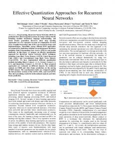
For the initial template in Eq. 25, the actual steady-state output images obtained by solving the di!erential equations in Eqs. 1}2 are identical to the external inputs in Fig. 1b. The OMER at the "rst step is equal to 298 which is the total number of mismatching pixels in the 5 images. The template values were changed by the RPLA with the positive constant learning rate g"0.0002. The actual output images at the second through "fth steps are obtained as in Fig. 1b. The actual output images in Fig. 1c, Fig. 1d, Fig. 1e, Fig. 1f and Fig. 1g are obtained at the 6th, 11th, 12th, 15th and 31th step, respectively. Since the actual outputs given in Fig. 1g match the desired outputs, then the OMER becomes zero and hence the RPLA stops at the 31th step. The "nal templates found are given in Eq. 24. These A*, B*, I* templates have been tested on 1 1 1 a test set consisting of the 50 16]16 input images not included by the training set. The learned templates failed to perform the edge detection with zero OMER for only a few images in the test set. The solution templates obtained by using 16]16 images in the training have good edge detection capability not only for 16]16 images but also for large images. In order to test validity of this claim, we experiment upon a binary Lenna image which is obtained by taking the most signi"cant bit for each pixel of the 256 gray-level Lenna image. The actual output of a 256]256 CNN with the templates A*, B*, I* is given in Fig. 2c. The image in 1 1 1 Fig . 2b is obtained by applying the well-known Canny's edge detector to the image in Fig. 2a. The same experiment is repeated for the chessboard image in Fig. 3. As can be observed from the "gures, CNNs with the learned templates perform as well as the Canny's edge detector. Experiments done on other real world images (e.g., house image) yielded similar results. However, these learned

305 Fig. 3a}c Test of the learned edge detection templates on chessboard. a Original chessboard image. b Image obtained by Canny's edge detector. c The actual output image of 256]256 CNN with templates A*, B*, I* 1 1 1

templates do not perform well for the noisy images (Yalc,mn and GuK zelis, 1996). In such cases, nonlinear templates can provide a solution. It is shown in Yalc,mn and GuK zelis, (1996) that, as a subclass of nonlinear B-template CNNs, radial-basis input function CNNs can be trained by a modi"ed version of RPLA and the learned nonlinear B-templates have quite satisfactory edge detection performance as well as for noisy binary images.

4.2 Corner detection

Fig. 2a}c Test of the learned edge detection templates on Lenna. a Original binary Lenna image. b Image obtained by Canny's edge detector. c The actual output image of 256]256 CNN with templates A*, B*, I* 1 1 1

The initial templates were chosen as in Eq. 25 which are the initial templates used also in the edge detection application. Figure 4a shows the initial images which are identical to the external images in Fig. 4b. The desired steady-state outputs are given in Fig. 4g. The RPLA was run by the positive constant learning rate g"0.0002. The actual steady-state outputs at the "rst through third steps are obtained with the OMER equal to 544 given in Fig. 4b, Fig. 4c, Fig. 4d, Fig. 4e, Fig. 4f and Fig. 4g shows the actual steady-state outputs at the 4th, 10}15th 19th, 28}29th and 48th steps, respectively. The "nal templates found at the end of the 48 iterations yield zero OMER for the 5 training samples used. These solution templates are given in Eq. 26.

306

Fig. 4a}g Learning corner detection. a The initial images, b the input images, c}f the actual output images at some intermediate steps, g the desired output images

307

Fig. 5 Learning hole "lling. a The initial images, b the input images, c}f the actual output images at several steps, g the desired output images

308

C C

!0.210844 !0.153426 !0.198075

w

D D

tion, corner detection, and hole "lling. The algorithm can be used for learning algebraic mappings from [!1, #1]m to M!1, #1Nm; but it has been observed that it is succesful in learning binary mappings.

A " !0.084514 3.331127 !0.084514 , 2 !0.198075 !0.153426 !0.210844 !0.345449 !0.450396 !0.349939 r w B " !0.510285 !0.583862 !0.510285 2 !0.349939 !0.450396 !0.345449

(26)

I*"!0.621101. 2

4.3 Hole "lling The initial templates were chosen as in Eq. 27.

C D C D 1 1 1

0 0 0

I0"0. 3

A0" 1 4 1 , B0" 0 4 0 , 3 3 1 1 1 0 0 0

(27)

Figure 5a shows the initial images. The external input images which are the input images fed to the CNN are given in Fig. 5b. The desired output images are shown in Fig. 5g. The RPLA was started by the initial templates in Eq. 27. The actual steady-state outputs at the "rst through third steps are same as the initial images in Fig. 5a. The OMER is decreased from 700 to 22 after 18 iterations. Whereas the OMER is 4 at the 26th step, it increases at 27th step to 22. Then, the OMER becomes 4 at the 32}34th steps, 22 to 35th step, 4 at the 36}48th steps, and falls to zero at the 49th step. Figure 5c, Fig. 5d, Fig. 5e, Fig. 5f and Fig. 5g shows the actual steady-state outputs at the 4th, 15}16th, 18}25th, 36}48th and 49th steps, respectively. The "nal templates found at the end of the 49 iterations yield zero OMER for the 5 training samples used. These solution templates are given in Eq. 28.

C C

0.498557 0.405644 0.527595

D D

A*" 0.519003 3.653047 0.519003 , 3 0.527595 0.405644 0.498557 0.060574 0.254369 0.118687

B*" 0.389894 4.346965 0.389894 , 3 0.118687 0.254369 0.060574

(28)

I*"!0.346954. 3

5 Conclusion Su$cient conditions for the recurrent perceptron learning algorithm for CNNs have been given. Also, the performance of the developed algorithm has been tested on learning some image processing tasks such as edge detec-

References Balsi M (1992) Generalized CNN: potentials of a CNN with nonuniform weights. 2nd IEEE Int Workshop of Cellular Neural Networks and their Appl, pp 129}134 Balsi M (1993) Recurrent backpropagation for cellular neural networks. European Conf on Circuit Theory and Design, pp 677}682 Chua LO, Shi BE (1991) Multiple layer cellular neural networks: a tutorial. In: Deprette F, der Veen AV (eds), Algorithms and Parallel VLSI Architecture, vol A, Elsevier, pp 137}168 Chua LO, Thiran P (1991) An analytical method for designing simple cellular neural networks. IEEE Trans on Circuits and Systems 38: 1332}1341 Chua LO, Yang L (1988) Cellular neural networks: theory and applications. IEEE Trans on Circuits and Systems 35: 1257}1290 Fajfar I, Bratkovic\ F, Tuma T, Puhan J (1998) A rigorous design method for binary cellular neural networks. Int J of Circuit Theory and Appl 26: 365}373 GuK nsel B, GuK zelis, C (1995) Supervised learning of smoothing parameters in image restoration by regularization under cellular neural networks framework. IEEE Int Conf Image Processing, pp 470}473 GuK zelis, C (1992) Supervised learning of the steady-state outputs in generalized cellular neural networks. 2nd IEEE Int Workshop on Cellular Neural Networks and their Appl pp 74}79 Guzelis, C, Chua LO (1993) Stability analysis of generalized cellular neural networks. Int J Circuit Theory and Appl 21: 1}33 GuK zelis, C, GuK nsel B (1995) Cellular neural networks for early vision. European Conf on Circuit Theory and Design, pp 785}788 GuK zelis, C, Karamahmut S (1994) Recurrent perceptron learning algorithm for completely stable cellular neural networks. 3rd IEEE Int Workshop on Cellular Neural Networks and their Appl pp 177}182 Karamahmut S, GuK zelis, C (1994) Recurrent back propagation algorithm for completely stable cellular neural networks. Turkish Symp on Arti"cial Intelligence and Neural Networks, pp 45}50 Kozek T, Roska T, Chua LO (1993) Genetic algorithm for CNN template learning. IEEE Trans on Circuits and Systems 40: 392}402 Liu D (1997) Cloning template design of cellular neural networks for associative memories. IEEE Trans on Circuits and Systems I 44: 646}650 Lu Z, Liu D (1998) A new synthesis procedure for a class of cellular neural networks with space-invariant cloning template. IEEE Trans on Circuits and Systems II 45: 1601}1605 Magnussen H, Nossek JA (1992) Towards a learning algorithm for discrete-time cellular neural networks. 2nd IEEE Int Workshop on Cellular Neural Networks and their Appl. pp 80}85 Nossek JA (1996) Design and learning with cellular neural networks Int J of Circuit Theory and Appl 24: 15}24 Nossek JA, Seiler G, Roska T, Chua LO (1992) Cellular neural networks: theory and circuit design. Int J of Circuit Theory and Appl 20: 533}553 Pineda FJ (1988) Generalization of backpropagation to recurrent and higher order neural networks. In: Anderson DZ (ed.), Neural information processing systems. American Inst of Phys, New York, 602}611 Rosenblatt F (1962) Principles of Neurodynamics. Spartan Books, New York Savacı FA, Vandewalle J (1993) On the stability analysis of cellular neural networks. IEEE Trans Circuits and Systems 40: 213}215

309 Schuler AJ, Nachbar P, Nossek JA, Chua LO (1992) Learning state space trajectories in cellular neural Networks. 2nd IEEE Int Workshop on Cellular Neural networks and their Appl, pp. 68}73 Schuler AJ, Nachbar P, Nossek JA (1993) State-based backpropagation-through-time for CNNs. European Conf on Circuit Theory and Design, pp. 33}38 Vanderberghe L, Vandewalle J (1989) Application of relaxation methods to the adaptive training of neural networks. Math Theory of Networks and Systems, MTNS'89, Amsterdam

Yalc,mn ME, GuK zelis, C (1996) CNNCs with radial basis input function. 4th IEEE Int Workshop on Cellular Neural Networks and their Appl pp 231}236 ZaraH ndy A (1999) The art of CNN template design. Int J of Circuit Theory and Appl 27: 5}23 Zou F, Schwartz S, Nossek JA (1990) Cellular neural network design using a learning algorithm. 1st IEEE Int Workshop on Cellular Neural Networks and their Appl. Amsterdam, pp 73}81